Discovery of 1–5 Hz flaring at high luminosity in SAX J1808.4–3658

Abstract

We report the discovery of a 1–5 Hz X-ray flaring phenomenon observed at $>30$ mCrab near peak luminosity in the 2008 and 2011 outbursts of the accreting millisecond X-ray pulsar SAX J1808.4–3658 in observations with the Rossi X-ray Timing Explorer. In each of the two outbursts this high luminosity flaring is seen for $\sim$3 continuous days and switches on and off on a timescale of 1–2 hr.

The flaring can be seen directly in the light curve, where it shows sharp spikes of emission at quasi-regular separation. In the power spectrum it produces a broad noise component, which peaks at 1–5 Hz. The total 0.05–10 Hz variability has a fractional rms amplitude of 20%–45%, well in excess of the 8%–12% rms broad-band noise usually seen in power spectra of SAX J1808.4–3658.

We perform a detailed timing analysis of the flaring and study its relation to the 401 Hz pulsations. We find that the pulse amplitude varies proportionally with source flux through all phases of the flaring, indicating that the flaring is likely due to mass density variations created at or outside the magnetospheric boundary. We suggest that this 1–5 Hz flaring is a high mass accretion rate version of the 0.5–2 Hz flaring which is known to occur at low luminosity ($<13$ mCrab), late in the tail of outbursts of SAX J1808.4–3658. We propose the dead-disk instability, previously suggested as the mechanism for the 0.5–2 Hz flaring, as a likely mechanism for the high luminosity flaring reported here.

1. Introduction

The accreting millisecond X-ray pulsar (AMXP) SAX J1808.4–3658 (henceforth SAX J1808), was the first X-ray binary to show pulsations in the millisecond domain (Wijnands & van der Klis, 1998). Since its discovery with the BeppoSax satellite in 1996 (in ’t Zand et al., 1998), SAX J1808 has shown regular outbursts with a recurrence time of 2–3.5 yr. Between 1998 and 2012 a total of 6 outbursts have been detected, all of which were extensively monitored with the Rossi X-ray Timing Explorer (RXTE). The light curves of these outbursts show a remarkably similar morphology (Hartman et al., 2008), consistently starting with a 2–5 day steep rise in flux (fast rise), followed by a flattening that lasts for a few days (peak). After reaching its peak X-ray luminosity, the light curve shows a slow exponential decay over a time span of several days (slow decay), followed by faster linear decay (fast decay) which typically lasts for 3–5 days (Hartman et al., 2008). After the fast decay, the source enters a prolonged, low luminosity state (outburst tail), during which $\sim$5 day long episodes of increased X-ray emission are seen (Patruno et al., 2009a), causing the luminosity to vary between $5\times 10^{32}$ and $5\times 10^{35}$ erg s^-1 (Wijnands, 2004; Campana et al., 2008). After several weeks to months, the outburst tail ends and the source returns to a quiescent luminosity of $\sim 5\times 10^{31}$ erg s^-1 (Heinke et al., 2009).

Several types of variability are seen in SAX J1808. The 401 Hz coherent pulsations can be detected throughout the outburst, including the outburst tail (Hartman et al., 2008, 2009; Patruno et al., 2012), and are thought to be caused by thermal emission from a localized region on the neutron star surface heated by the impact of plasma coming down the accretion funnel. This so-called hotspot revolves with the neutron star spin, modulating the observed X-ray flux at the spin frequency. The pulsations thus offer a physical tracer of the innermost accretion flow.

In addition to the pulsations, type I X-ray bursts (in ’t Zand et al., 1998) and twin kHz quasi-periodic oscillations (QPOs; Wijnands et al., 2003) have also been detected in SAX J1808. The stochastic variability of the 1998 and 2002 outbursts of SAX J1808 has been studied by van Straaten et al. (2005), who find that the power spectral characteristics are similar to those of a typical atoll source.

A peculiar type of variability in SAX J1808 is the strong 0.5–2 Hz flaring often seen in the outburst tail at luminosities $<13$ mCrab. This phenomenon has frequently been designated as the ‘1 Hz QPO’, however, in this paper we refer to it as the ‘low luminosity flaring’. The low luminosity flaring was first reported by van der Klis et al. (2000) and found to occur sporadically throughout the outburst tails of 2000 and 2002 (Wijnands, 2004). An in-depth study by Patruno et al. (2009a) showed that it was also present in the tail of the 2005 outburst, but not in the tail of the 2008 outburst. In the later 2011 outburst the low luminosity flaring was again not detected (Patruno et al., 2012), although due to Solar constraints only the onset of the tail could be observed.

The large luminosity variations in the outburst tails of SAX J1808 have been proposed to be caused by an intermittent propeller effect (Campana et al., 2008). In the propeller regime the inner edge of the accretion disk rotates slower than the neutron star magnetosphere and in-falling matter is no longer able to accrete onto the neutron star, but instead is blown out of the system as by a propeller (Illarionov & Sunyaev, 1975). Considering the 0.5–2 Hz low luminosity flaring in the context of the propeller onset, Patruno et al. (2009a) propose the Spruit–Taam instability (Spruit & Taam, 1993) as the most likely origin. An open problem with this interpretation, however, is the sporadic nature of this flaring in the 2000, 2002 and 2005 outburst tails as well as its complete absence in the 2008 and 2011 outbursts. As noted by Patruno et al. (2009a) other mechanisms such as an interchange instability (Arons & Lea, 1976) can not be strictly ruled out.

In the present work we report on the detection of strong 1–5 Hz flaring observed in the 2008 and 2011 outbursts of SAX J1808 that is similar to the 0.5-2 Hz low luminosity flaring, but occurs at much higher luminosities, near the peak of the outburst. We present the timing properties of this high luminosity flaring and discuss its nature. In Section 2 we outline our data reduction procedure and our timing analysis methods. In Section 3 we present the results we obtained and in Section 4 we explore potential mechanisms for the high luminosity flaring and discuss our results in the context of the previously observed low luminosity flaring. Our conclusions are summarized in Section 5.

2. X-ray Observations

We used data collected with the RXTE Proportional Counter Array (PCA, see Jahoda et al., 2006, for technical details). For the timing analysis we used the pointed observations of all observed outbursts of SAX J1808, excluding the outburst tail, selecting only data taken in GoodXenon or 122 $\mu$s Event mode. All data were binned to a time resolution of 1/8192 s prior to further analysis.

Additionally, we used the 16 s time-resolution Standard-2 data to construct 2–16 keV X-ray light curves normalized to Crab and calculate the standard Crab-normalized soft (3.5–6.0 keV / 2.0–3.5 keV) and hard (9.7–16 keV / 6.0–9.7 keV) colors (see e.g. van Straaten et al., 2003, for the detailed procedure).

2.1. Stochastic Timing Analysis

To study the stochastic time variability we calculated Fourier transforms of 256 s data segments, giving a frequency resolution of $\sim 4\times 10^{-3}$ Hz and a Nyquist frequency of 4096 Hz. To optimize the signal-to-noise we selected only the events in channels 5–48 ($\sim$2–20 keV). No background subtraction or dead-time correction was applied prior to the Fourier transform. We used the transforms to compute Leahy normalized power spectra and subtracted the Poisson level using the formula of Zhang et al. (1995) according to the method described by Klein-Wolt et al. (2004).

Power spectra computed using segments of the same ObsID were averaged to improve statistics. Additionally, power spectra of consecutive ObsIDs were sometimes averaged to improve statistics further, but only if their flux and color properties were consistent with being the same and the power spectra were similar.

Finally, we normalized the averaged power spectra to source fractional rms amplitude squared per Hz while correcting for the background count rate as estimated using the ftool pcabackest (van der Klis, 1995). In this normalization the fractional rms contribution, $r$, of a given frequency band is

$$r^{2}=\int_{\nu_{1}}^{\nu_{2}}P(\nu)d\nu,$$ (1)

where $P(\nu)$ is the power density in the described units.

We describe the power spectra by fitting a function consisting of the sum of several Lorentzians plus a Schechter function for the flaring component (see Section 3). We characterize each Lorentzian by its centroid frequency and full-width-at-half-maximum (FWHM). The strength, or power, of the Lorentzian is obtained by integrating it over frequency from 0 to $\infty$ and reported in terms of the corresponding fractional rms as defined in equation 1.

The Schechter function is an exponentially cut-off power law and is given by $P(\nu)\propto\nu^{-\alpha}e^{-\nu/\nu_{cut}}$ (Hasinger & van der Klis, 1989; Dotani et al., 1989), with power-law index $\alpha$ and cut-off frequency $\nu_{cut}$. We can define a ‘centroid’ frequency $\nu_{0}=-\alpha\nu_{cut}$ as the frequency at which the Schechter function reaches is maximum in $P(\nu)$.

2.2. Coherent Timing Analysis

We correct the photon arrival times to the solar system barycenter with the ftool faxbary using the source coordinates of Hartman et al. (2008). This tool also applies the RXTE fine clock corrections, allowing for high precision ($\sim$4 $\mu$s) timing analysis (Rots et al., 2004). Selecting only the events in the channel range 5–37 ($\sim$2–16 keV) (Patruno et al., 2012), we fold the data to produce folded pulse profiles. For the timing solution we use the ephemeris of Hartman et al. (2009) for the 2008 outburst and that of Patruno et al. (2012) for the 2011 outburst. The length of the folded data segments varies depending on purpose; typically we fold $\sim$3000 s of continuous RXTE observations to obtain high signal-to-noise pulse profiles. Alternatively we take $\sim$256 s segments to obtain better time resolution when following the outburst evolution. In both cases we allow the segment length to vary such that we use the entire observed time series.

3. Results

The outbursts of SAX J1808 show very similar light curves. In Figure 1 we show the four outbursts that occurred between 2002 and 2011. Since the 1998 outburst does not show either flaring component and in 2000 only the outburst tail could be observed, we do not show these outbursts and exclude them from further analysis.

In Figure 1 the light curves where shifted in time such that the transition from the slow decay to the fast decay occurs on day 15. The top panels indicate the times of confirmed and suspected X-ray bursts (removed from the data prior to the analysis), detections of the low luminosity flaring (Patruno et al., 2009a) and detections of the high luminosity flaring (below).

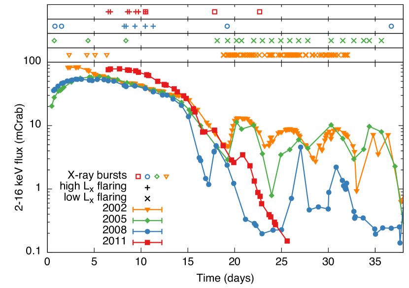
Figure 1.— Light curves in the 2–16 keV X-ray band of the 2002 (orange triangles), 2005 (green diamonds), 2008 (blue circles) and 2011 (red squares) outbursts. The symbols in the top bars show the times of type I X-ray bursts and observations with high luminosity flaring (pluses, this paper) and low luminosity flaring (crosses, Patruno et al., 2009a). The light curves have been shifted in time such that the transition from slow to fast decay is at day 15, using a shift in MJD of 52553.6, 53522.3, 54731.2 and 55863.4 for the outbursts 2002 through 2011, respectively.

Like the light curves, the power spectra of SAX J1808 are similar. The power spectra can usually be described with 4 Lorentzians (van Straaten et al., 2005); a broad noise ‘break’ component at $\sim$4 Hz, a ‘hump’ component in the range $\sim$20–80 Hz, a hectoHz component in the range $\sim$100–200 Hz, and the upper kHz QPO with a frequency in the range $\sim$300–700 Hz.

Both in 2008 and 2011 we find an interval spanning $\sim$3 days during which the power spectrum deviates significantly from its standard shape. The power density between 0.05 Hz and 10 Hz is much higher and rather than showing the usual horizontal plateau in $P(\nu)$, the power density shows a peak around $\sim$3 Hz (see Figure 2). Lorentzian and Gaussian functions fail to provide statistically acceptable fits to the power spectra as they are not steep enough at low frequencies. We find that replacing the Lorentzian break component with a Schechter function does provide a satisfactory fit to the data. The observations in which we see this behavior are marked with pluses in Figure 1 and their ObsIDs are given in Table 1. We combined the 12 observations showing this new phenomenon into 8 intervals and give all power spectrum fit parameters for those intervals in Table 2.

Table 1 High Luminosity Flaring Observation Information

ObsID	Length (s)	Start MJD	Flux (mCrab)	rms (%)a
2008 Outburst
A-07	3000	54739.40	43.2	28.5
A-09	2300	54739.60	41.4	29.0
A-02	6100	54740.54	42.2	27.0
A-08	6100	54741.65	38.5	29.0
B-00b	1280	54742.49	34.1	38.7
2011 Outburst
C-01	2800	55869.83	76.3	21.9
C-00	12000	55870.16	78.2	21.7
C-02	6100	55871.13	78.8	11.1
C-03	5400	55871.98	75.7	22.4
C-04	6100	55872.18	74.7	22.1
C-05	3100	55872.86	73.2	18.9
C-06	6100	55873.16	69.5	22.3

Note. — A = ObsID 93027-01-02, B = ObsID 93027-01-03, C = ObsID 96027-01-01.

Table 2 Power Spectrum Fit Parameters

	high $L_{x}$ flaring	Hump	hHz	upper kHz
	$\alpha$	FWHM	FWHM	FWHM
Group	$\nu_{cut}$	$\nu_{0}$	$\nu_{0}$	$\nu_{0}$	$\chi^{2}$/dof
	$r$	$r$	$r$	$r$
2008
	$-0.69\pm 0.04$	$45.6\pm 4.9$	$\cdots$	$404\pm 196$
A-07, A-09	$2.54\pm 0.12$	$21.4\pm 2.8$	$\cdots$	$496\pm 56$	173/118
	$28.03\pm 0.43$	$29.1\pm 1.8$	$\cdots$	$19.5\pm 3.1$
	$-0.41\pm 0.02$	$46.7\pm 4.1$	$\cdots$	$147\pm 103$
A-02	$4.21\pm 0.15$	$34.1\pm 1.7$	$\cdots$	$618\pm 31$	148/121
	$28.72\pm 0.29$	$26.0\pm 1.0$	$\cdots$	$12.1\pm 2.3$
	$-0.51\pm 0.05$	$60.1\pm 9.7$	$\cdots$	$\cdots$
A-08	$3.59\pm 0.24$	$29.2\pm 6.5$	$\cdots$	$\cdots$	76.8/121
	$30.78\pm 0.66$	$28.6\pm 2.7$	$\cdots$	$\cdots$
	$-1.94\pm 0.25$	$14.1\pm 3.2$	$\cdots$	$\cdots$
B-00	$1.40\pm 0.19$	$9.1\pm 1.6$	$\cdots$	$\cdots$	102/75
	$34.4\pm 1.6$	$25.7\pm 2.7$	$\cdots$	$\cdots$
2011
	$-0.45\pm 0.01$	$40.8\pm 3.1$	$427\pm 232$	$72\pm 23$
C-01, C-00	$5.63\pm 0.09$	$44.64\pm 0.52$	$199\pm 164$	$656.1\pm 2.3$	172/141
	$25.48\pm 0.10$	$20.20\pm 0.92$	$16.7_{-2.3}^{+11.2}$	$11.54\pm 0.76$
	$-0.79\pm 0.15$	$58\pm 18$	$\cdots$	$494\pm 430$
C-02	$5.65\pm 0.95$	$24\pm 13$	$\cdots$	$466\pm 118$	58.9/65
	$15.4\pm 1.3$	$13.7\pm 3.3$	$\cdots$	$12.9\pm 3.8$
	$-0.55\pm 0.02$	$52.0\pm 3.3$	$151\pm 50$	$95\pm 17$
C-03, C-04	$5.29\pm 0.11$	$46.4\pm 1.1$	$321\pm 24$	$716.0\pm 4.6$	228/123
	$26.75\pm 0.15$	$21.48\pm 0.54$	$8.8\pm 1.2$	$13.34\pm 0.64$
	$-0.59\pm 0.02$	$31.3\pm 4.6$	$472\pm 255$	$61\pm 37$
C-05, C-06	$5.80\pm 0.13$	$50.04\pm 0.82$	0 (fixed)	$709.3\pm 3.3$	140/124
	$27.31\pm 0.18$	$16.0\pm 1.4$	$21.6\pm 1.9$	$12.60\pm 0.74$

Note. — A = ObsID 93027-01-02, B = ObsID 93027-01-03, C = ObsID 96027-01-01. Frequencies $\nu_{0}$ and $\nu_{cut}$ and FWHM are in units of Hz, and fractional rms, r, is expressed as a percentage.

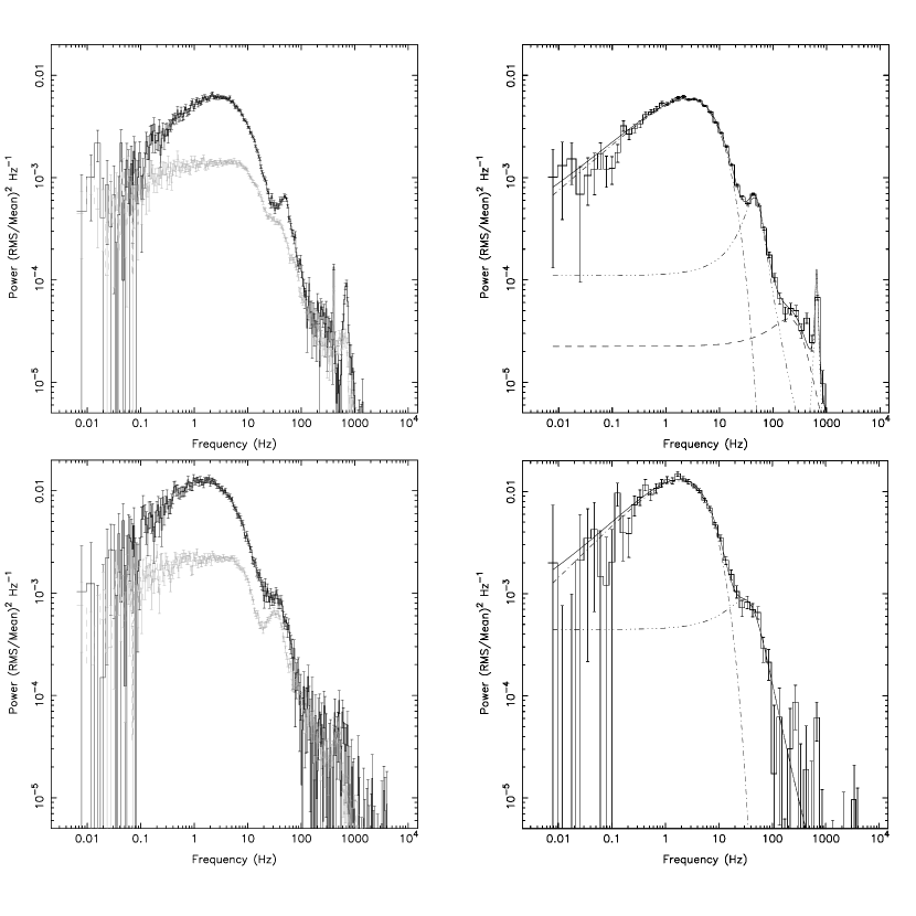
Figure 2.— Power spectra of the high luminosity flaring. The left column compares the high luminosity flaring (average of all ObsIDs reported Table 1) of 2011 (top, black) and 2008 (bottom, black) with the broad band noise in the 2002 (top, gray) and 2005 (bottom, gray) outbursts in similar outburst stages and spectral states. The right column shows the Schechter function fit to power spectra for the 2011 (top) and 2008 (bottom) outbursts. Note that all power spectra show power density versus frequency.

The centroid frequency of the best-fit Schechter function, as defined in Section 2.1, varies between 1 and 5 Hz. The amplitude of the flaring varies between 26% and 34% rms, and shows a clear anti-correlation with $\nu_{0}$ (see Figure 3). The power-law index $\alpha$ shows some scatter, but no correlation with frequency.

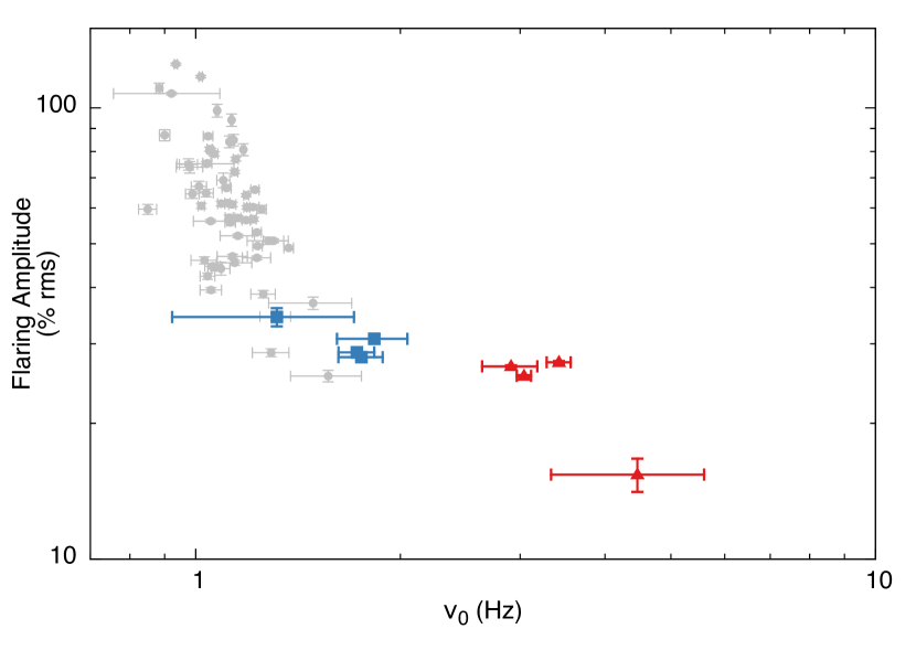
Figure 3.— Correlation between the fractional rms and the high and low luminosity flaring centroid frequencies. We show the 2008 (blue squares) and 2011 (red triangles) high luminosity flaring frequency obtained in this work along with the low luminosity flaring frequencies (grey) from (Patruno et al., 2009a) against their respective fractional rms.

The morphology of this new component is very different from the regular broad band noise, but quite similar to that of the low luminosity flaring seen in the outburst tails. Because the power spectrum returns to its normal shape outside the reported $\sim$3 day intervals, we suggest that this new high luminosity flaring phenomenon dominates over the Lorentzian break component normally seen in the same frequency range. During the 2008 outburst the amplitude of this new component briefly reaches $\sim$45% rms (see Section 3.1). In the bottom panel of Figure 4 we show a small selection of the light curve during this time. The $\sim$3 Hz variability is directly visible and indeed has a flaring morphology, showing relatively sharp spikes of emission at quasi-regular separation. Contrary to the 0.5–2 Hz low luminosity flaring, which is seen only in the outburst tail for luminosities $<13$ mCrab, the 1–5 Hz flaring, reported here for the first time, occurs near the peak of the outburst at luminosities $>30$ mCrab and is therefore called the high luminosity flaring.

Figure 4.— Light curve segments of the 2008 outburst at a time resolution of 0.035 s. The top panel shows a segment of ObsID 93027-01-03-02 which shows the regular broad band noise in the power spectrum. The bottom panel shows a segment of ObsID 93027-01-03-00, during the time that the high luminosity flaring shows an amplitude of 45% rms.

In order to study the evolution of the high luminosity flaring on short time scales we compute power spectra of 256 s data segments. Fitting a Schechter function to these short segment power spectra does not provide meaningful results, so instead we characterize the high luminosity flaring power by integrating the power spectrum between 0.05 and 10 Hz, the range in which we observe the bulk power in excess of the expected break component. These frequency bounds are identical to those used by Patruno et al. (2009a), allowing a comparison of the low luminosity flaring results with the results we obtain for the high luminosity flaring. The power estimates obtained in this way are described below. They match with the power measured by fitting a Schechter function to power spectra of longer observations.

We also study the relation of the high luminosity flaring with the 401 Hz pulsations by constructing pulse profiles for the same data segments and considering the joint behavior of the flaring rms amplitude and the phase and amplitude of the pulsations. We now discuss these results in detail for each outburst.

3.1. 2008

In 2008 the high luminosity flaring is seen at the onset of the slow decay. The flaring is present for $\sim$3.1 days between MJD 54739 and MJD 54742, during which the flux decays from 43 to 34 mCrab. In Figure 5 we present the source evolution during this interval showing, from top down, the 2–16 keV light curve, hard (orange) and soft (purple) colors, 0.05–10 Hz rms amplitude, and the phase and amplitude for the fundamental (blue) and second harmonic (red) of the 401 Hz pulsations. In the left column we averaged the data segments per $\sim 3000$ s RXTE observations and the right column uses the full 256 s resolution. We describe the evolution as a function of days using the time shift of Figure 1.

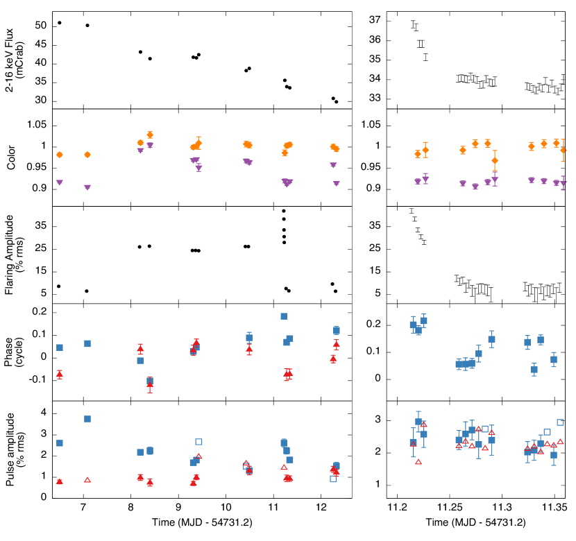
Figure 5.— Evolution of the high luminosity flaring in the 2008 outburst, showing in the left column: the 2–16 keV light curve (top panel); soft (purple triangle) and hard (orange diamond) colors (second panel); 0.05–10 Hz high luminosity flaring fractional rms (middle panel); the pulse phases (fourth panel) and finally the pulsed fractional rms (bottom panel). Amplitude and phase measurements of the pulsations are given for the fundamental (blue squares) and the second harmonic (red triangles). Open symbols give 95% confidence upper limits. The right column shows the same data, but zoomed in on the flaring switch-off.

The flaring is first observed at day 8.3 with a fractional rms of 28%. The previous observation $\sim$1.1 days earlier, showed a fractional rms of 8%. Assuming this level of fractional variability due to the break component persists incoherently during the flaring interval, an rms amplitude of 27% is deduced for the flaring.

Between day 8.3 and 10.3 the flaring amplitude varies between 25% and 28% rms, showing a weak anti correlation with flux on a day-to-day timescale. In the same period the soft color slowly decreases while the hard color remains roughly constant. Since these color trends extend beyond the flaring interval, and are also seen in the same stage in the other outbursts (van Straaten et al., 2005), they are most likely not related to the presence of flaring. During the flaring interval the pulse amplitude and phase show complicated variations, again also seen outside the flaring interval and in the other outbursts (see e.g. Hartman et al., 2008), which relate to the flux variations rather than the presence of flaring (Patruno et al., 2009b).

At day 11.3 we see the flaring at an amplitude of 45% before it switches off. During the switch-off we see the flaring rms drop dramatically over the course of 5 consecutive data segments, showing a strong correlation with a small drop flux. A zoom-in of this entire episode is shown in the right column of in Figure 5. Assuming the flaring started to switch off at the highest observed fractional rms and completely turned off at day 11.27, we obtain a switch-off time of 1.2 hr. Since the decay could have set in prior to the observed peak this is a lower limit.

While the flaring rms amplitude drops rapidly, the pulse fundamental remains steady in amplitude and phase. Yet, at day 11.27, just as the fractional rms returns to the 8% base level, there is a systematic drift in the fundamental phase of about 0.1 cycles, which is does not relate to a flux variation and might be a response to the flaring mechanism.

3.2. 2011

In Figure 6 we show the outburst evolution during the flaring interval of the 2011 outburst. In the first observation of the 2011 outburst, at MJD 55869.9, the flaring is already present with a 0.05–10 Hz rms of $\sim 23\%$. The flaring stays active for the following 4 days, during which the flux decays from $76$ to $69$ mCrab.

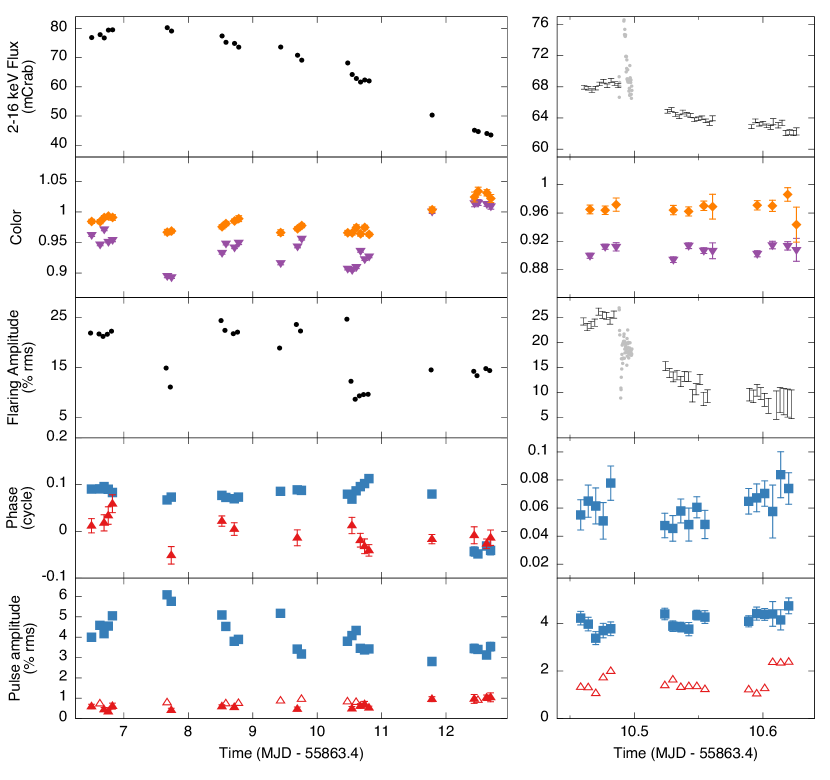
Figure 6.— Evolution of the high luminosity flaring in the 2011 outburst in comparison to the 401 Hz pulsations. The grey bullets in the right column show the flux and 0.05–10 Hz fractional rms of 16 second data segments during a type I X-ray burst interval. For a detailed view see Figure 7. For details on the remaining data see Figure 5.

At day 7.9 the flaring decreases in strength, with the amplitude dropping consecutively to $\sim 15\%$ and $\sim 9\%$ rms. The rms drop coincides with the outburst peak luminosity, and an unexpected drop in soft color. At the same time the pulsations show a drop in the second harmonic phase and an increase in the fundamental amplitude, however, this could again be related to the flux rather than the flaring.

Over the entire flaring interval, between days 6.5 and 10.5, the flaring rms varies between 17% and 26%, showing a correlation with flux on a 3000 s timescale and an anti-correlation on the longer day-to-day timescale.

At day 10.49 a bright type I X-ray burst occurs (in ’t Zand et al., 2013). Prior to the X-ray burst the flux is constant and the flaring amplitude holds steady at 25% rms (see Figures 6 and 7). During the X-ray burst peak flux ($\sim 7$ Crab) there is no significant variability in the 0.05–10 Hz frequency band above the Poisson noise level, giving a 95% confidence level upper limit on the flaring amplitude of 2% rms. As the burst flux decays, the 0.05–10 Hz fractional rms slowly increases, such that the absolute rms is consistent with the pre-burst level. At 550 s after the X-ray burst went off, just before the end of the RXTE observation, the flux returns to its pre-burst level, but at 18% rms the flaring amplitude does not.

In the next RXTE observation, at day 10.52, the flaring amplitude is 15% rms, and shows a steady decrease until it reaches the 8% rms of the broad band noise on day 10.6 . Outside the X-ray burst interval, the switch-off is again strongly correlated with a small drop in flux. Assuming the switch-off started when the X-ray burst occurred, we obtain a switch-off time of $\sim 2$ hr. Like in the 2008 outburst, the pulse fundamental phase shows a systematic drift of 0.1 cycles after the flaring switched off, although for the 2011 outburst this drift is much slower.

Figure 7.— Evolution of the 2–16 keV X-ray flux (top, second), the 0.05–10 Hz fractional rms (third) and absolute rms (bottom) of the 2011 type I X-ray burst in seconds since the start of the burst. The open symbols in the third panel give 95% C.L. upper limits on the fractional rms. The corresponding upper limits on the absolute rms where greater than 50 mCrab and have been omitted for clarity. Horizontal dashed lines show the respective averaged pre-burst levels.

3.3. Summary of Observed Correlations

The sharp decrease in flaring amplitude when the flaring switches off in both outbursts and the rms drop at peak flux in 2011 suggest the flaring only occurs in a specific flux range with a sharp upper and lower bound which differs between the two outbursts. The flaring switch-off takes place on a timescale of 1–2 hr and is strongly correlated with flux. In one outburst the start of the flaring switch-off coincides with a bright type I X-ray burst.

Directly after the flaring switches off and the 0.05–10 Hz rms returns to the 8% rms of the broad band noise, the pulse phase of the fundamental shows a systematic drift of 0.1 cycles for both outbursts.

For both outbursts the flaring fractional amplitude correlates with flux on a 3000 s timescale, while on a longer day-to-day timescale the flaring fractional amplitude is anti-correlated with flux. If we consider the relation of the 0.05–10 Hz fractional rms versus mean flux in the 2002 and 2005 outbursts, we find that the broad band noise follows similar trends, but with different correlation factors, indicating the observed relations between flux and flaring rms are not due the underlying broad band noise. This supports our assumption that the flaring is a distinct component that is added onto the broad band noise.

3.4. Relation of the Flaring Phase with Pulsations

In ObsID 93027-01-03-00 (day 11.2 of the 2008 outburst) the flaring reached an rms of 45% and was directly visible in the light curve (Figure 4). This allows us to investigate the pulsations as a function of the flux variations at the flaring timescale.

We construct a light curve at 1/32 s time resolution and sort the light curve in flux quartiles. To account for longer timescale variations in flux we apply the quartile selection on short 8 s segments containing 256 flux estimates. We then construct 4 pulse profiles corresponding to the the 4 flux quartiles. We find that the pulse phases in different quartiles are statistically consistent. The absolute amplitude of the pulsations is found to be proportional to flux ($\chi^{2}/\mbox{dof}=0.6$), such that the fractional amplitudes are the same within the errors (see Table 3).

Table 3 Pulse Parameters for Quartile Selection

Count rate	Pulse Amplitude (% rms)	Error	Phase	Error
70.6	2.55	0.83	0.27	0.05
138.3	2.09	0.57	0.30	0.04
193.1	2.53	0.39	0.26	0.02
314.8	2.93	0.33	0.30	0.02

3.5. Energy Dependence

Figure 8 shows the energy dependence of the high luminosity flaring fractional rms as measured in the 0.05–10 Hz band. We consider the fractional rms, which means the rms spectrum is divided by the energy spectrum of the mean flux. If the flaring has the same energy dependence as the mean flux, then we expect the fractional rms to be constant in energy at the level of the fractional rms of the full energy band. We find that the rms energy spectrum deviates from the average spectrum by contributing more between 6–16 keV and less below 6 keV.

This harder-than-average spectrum suggests that the high luminosity flaring does not originate from the soft disk emission, but instead comes from a harder spectral component, possibly the neutron star surface or boundary layer (Gilfanov et al., 2003).

We observe the same fractional rms spectral shape for the flaring during both the 2008 and 2011 outbursts. More importantly, in this frequency range the same rms spectral shape is also found for observations where the flaring is not seen, which suggests that the broad band noise in the 0.05–10 Hz range and the flaring share a similar origin. Since the broad band noise is believed to be caused by mass accretion rate variations in the inner accretion disk, this suggests that the high luminosity flaring is an accretion rate variation as well.

Figure 8.— Fractional rms spectra for flaring (right) and non-flaring (left) intervals in the 2011 outburst. We show the fractional rms divided by the mean fractional rms of the full energy band (22.1% and 13.3%, respectively).

4. Discussion

We have found two intervals of unusual 1–5 Hz flaring occurring at high luminosity ($>30$ mCrab) in the 2008 and 2011 outbursts of SAX J1808 as observed with RXTE. This high luminosity flaring is characterized by spikes of emission in the light curve at quasi-regular intervals, which result in a broad noise component in the power spectrum. It is only seen for 3–4 days per outburst in a narrow $\sim$10 mCrab wide flux window at a different flux for 2008 and 2011, and only in those 2 (of 6) outbursts.

The characteristics of the high luminosity flaring are reminiscent of those of the low luminosity ($<13$ mCrab) flaring previously detected in the tail of the of 2000, 2002 and 2005 outbursts (Patruno et al., 2009a). The low luminosity flaring also produces a broad noise component in the power spectrum and is also seen exclusively in a narrow $\sim 10$ mCrab wide flux window, which, however, is at the same flux for all three outbursts. The high and low luminosity flaring also differ in a number of other ways. Specifically, the high luminosity flaring is seen at $\sim$35 and $\sim$75 mCrab, with centroid frequency, $\nu_{0}$, of 1–5 Hz and rms amplitudes of 20–45%. The low luminosity flaring, on the other hand, is seen between 2 and 13 mCrab, with $\nu_{0}$ of 0.5–2 Hz and rms amplitudes between 40% and 120%. As seen in Figure 3 the trend in fractional rms against frequency of the high and low luminosity flaring match at $\sim$40% rms, but the relation is different for the two types of flaring. Additionally, the absolute rms increases with frequency.

The similarities between the high and low luminosity flaring suggest they could be caused by the same mechanism, however, the large discrepancy in the luminosity at which they are detected might indicate the opposite. We therefore first consider mechanisms that can explain the properties we observe for the high luminosity flaring alone, then we consider models that could explain them commonly with the low luminosity flaring.

4.1. Flaring Origin

The observed flaring can either be caused by an extra emission component from the accretion disk or neutron star; or by periodic obscuration along the line of sight or a variation in the accretion flow.

4.1.1 An Isolated Component

In both the 2008 and 2011 outbursts the flaring switched off smoothly, showing a strong correlation between a drop in flux and the decreasing flaring amplitude. This correlation might suggest that the flaring is due to some isolated emission component that is added to the mean flux. For such a process, we can estimate an upper limit on fractional rms of the total signal by assuming the extra component is 100% modulated. We consider a signal of the form $f(t)=a+p(t)$, such that $a$ gives the unperturbed flux and $p(t)$ the added flaring signal. The average of $f(t)$ is $\mu_{f}=a+\mu_{p}$ with $\mu_{p}$ the average of $p(t)$. The fractional rms of the total signal is defined as

$$r=\frac{\mbox{rms}}{\mu_{f}}=\frac{\sqrt{\int_{0}^{T}(f(t)-\mu_{f})^{2}dt/T}}{\mu_{f}},$$ (2)

with $T$ the average period of a single flare. For simplicity we take p(t) to be a square wave with duty cycle $D$, such that wave amplitude is $\mu_{p}/D$. The enumerator now reduces drastically, giving

$$r=\sqrt{D^{-1}-1}\ \frac{\mu_{p}}{\mu_{f}}.$$ (3)

For $\mu_{f}$ we can use the observed flux prior to switch-off, which is 37 and 68 mCrab for 2008 and 2011 respectively. The flux drop during the switch-off gives $\mu_{p}$, which is 3 mCrab in both outbursts. To calculate the minimum required duty cycle we use the maximum observed fractional rms (45% and 26%, respectively) and find that a duty cycle of $\sim 0.03$ is needed. This is much higher than the $D\simeq 0.25$ that is apparent in the light curve (see e.g. Figure 4), so the flaring cannot be produced by an isolated emission process.

4.1.2 Surface Processes

In Section 3.4 we found that the pulse amplitude responds to flux variations due to individual flares. This might suggest that the flaring originates from the neutron star surface, for instance from QPOs on the nuclear burning timescale in the hotspot (see e.g. Bildsten, 1998; Heger et al., 2007).

Marginally stable nuclear burning occurs in the transition between stable and unstable burning. It therefore occurs only in a narrow range of mass accretion rates, naturally explaining the narrow flux window observed for the high luminosity flaring. Furthermore, a transition to unstable burning, a type I X-ray burst, should stop the flaring, which is indeed observed during the 2011 flaring switch-off.

The predicted oscillation timescale of marginally stable burning depends on the thermal and accretion timescale of the burning region and is $\sim 100$ s (Heger et al., 2007), which is too slow to account for the observed flaring. Furthermore, the flux variation due to the oscillations is limited by the fraction of nuclear energy and gravitational energy released per accreted nucleon. This fraction is of the order of a few percent, resulting in a fractional rms of $\sim 5-10\%$ (depending on duty cycle, see equation 3), far too low to account for the large fractional amplitude of the high luminosity flaring. Nuclear burning therefore is an unlikely candidate.

4.1.3 Obscuration

Another possibility is that the flaring is caused by periodic obscuration of the neutron star. Dipping low-mass X-ray binaries show QPOs in the $\sim$0.5–2.5 Hz range at rms amplitudes up to 12% (Homan et al., 1999; Jonker et al., 1999, 2000). These QPOs were proposed to be caused by a nearly opaque medium orbiting at the radius where the orbital frequency matches the observed QPO frequency. This argument is supported by the flat rms spectrum of the QPO, the high inclination angle of the binaries, and constant fractional rms amplitude during short term luminosity variations like dips and type I X-ray bursts, which are all characteristics of obscuration.

The frequency range of the dipping QPO is similar to that of the high luminosity flaring, but all other characteristics differ. SAX J1808 does not show dips in the light curve and at an inclination of $60^{\circ}$ (Cackett et al., 2009; Ibragimov & Poutanen, 2009; Kajava et al., 2011) is unlikely to show obscuration. The rms spectrum of the flaring is not flat, and the flaring fractional rms is diluted by the increased flux on a type I X-ray burst. An obscuration origin for the high luminosity flaring can therefore be ruled out.

4.1.4 Accretion Flow Variations

The rms spectrum (Section 3.5) suggests the high luminosity flaring may be due to variations in the accretion flow. If this is the case, flaring variability is present in the accretion flow channeled to the hotspot, and should therefore affect both the persistent emission and the pulsed emission in a similar fashion. This relation between the flares and the pulsations was indeed observed (see Section 3.4). As, therefore, the accretion flow is the most plausible origin for the high luminosity flaring, we consider a number of such mechanisms in greater detail.

4.2. Disk Length- and Timescales

We discuss instabilities in the accretion flow within the framework of the interplay between the corotation and magnetospheric radius. The corotation radius, $r_{c}$, is defined as the radius where the disk Keplerian frequency matches the neutron star spin frequency and the magnetospheric radius, $r_{m}$, as the radius where magnetic stresses equal the material stresses of the accreting plasma. For specificity we note that $r_{c}$ can be written as

$$r_{c}\simeq 31\left[\frac{\nu_{s}}{400\mbox{ Hz}}\right]^{-2/3}\left[\frac{M}{1.4M_{\odot}}\right]^{1/3}\mbox{ km},$$ (4)

with $\nu_{s}$ the spin frequency and $M$ the neutron star mass. Additionally we write $r_{m}$ as (Spruit & Taam, 1993; D’Angelo & Spruit, 2010)

$$r_{m}\simeq 20 \left[\frac{M}{1.4M_{\odot}}\right]^{-1/10}\left[\frac{B}{10^{8}\mbox{ Gauss}}\right]^{2/5}\left[\frac{R}{10\mbox{ km}}\right]^{6/5}$$ (5)

$$\times\left[\frac{\dot{M}}{4\times 10^{-10}M_{\odot}\mbox{yr}^{-1}}\right]^{-1/5}\left[\frac{\nu_{s}}{400\mbox{ Hz}}\right]^{-3/10}\mbox{ km},$$

where $B$ is the magnetic field strength, $R$ the neutron star radius and $\dot{M}$ the mass accretion rate.

In 2008 the high luminosity flaring is seen at an average flux of $F=41$ mCrab. Relating flux to mass accretion rate as $4\pi d^{2}F=GM\dot{M}/R$, for a distance $d=3.5(1)$ kpc (Galloway & Cumming, 2006), and bolometric correction factor of 2.14 (Galloway et al., 2008), the mass accretion rate was $3\times 10^{-10}M_{\odot}$ yr^-1 during the high luminosity flaring in the 2008 outburst. In 2011 the high luminosity flaring appears at an average flux of $75$ mCrab, giving a mass accretion rate of $5\times 10^{-10}M_{\odot}$ yr^-1. For a canonical accreting neutron star ($M=1.4M_{\odot}$, $R=10$ km and $B=10^{8}$ Gauss), we find an $r_{m}$ of $\sim$21 km and $\sim$19 km for 2008 and 2011, respectively.

As a second estimate of the inner disk radius we can assume the upper kHz QPO frequency (see Table 2) to be a proxy for the inner disk Kepler frequency. This way we obtain radii of 21–28 km. All these estimates are consistent with an inner disk cut off by the magnetosphere near the corotation radius.

4.3. Magnetic Reconnection

Magnetic reconnection has been proposed by Aly & Kuijpers (1990) as the origin of QPOs that occur in the Rapid Burster at frequencies similar to those in SAX J1808 discussed here. In their magnetic reconnection model the stellar magnetic field threads the inner disk. The differential rotation between the accretion disk and the magnetosphere shears the field lines, building up magnetic energy. This energy is periodically released in reconnection events that occur a few times per beat period between the inner edge of the accretion disk and the neutron star spin. The reconnection events break up the accretion flow into blobs, which results in the observed flaring behavior.

Because in this model the QPO frequency depends on the beat between the inner disk radius and the neutron star spin, it will be a function of mass accretion rate. An increasing mass accretion rate pushes the disk inward. For $r_{m}>r_{c}$ this causes a decreasing QPO frequency, at $r_{m}=r_{c}$ the QPO frequency passes through zero, and for $r_{m}<r_{c}$ the frequency will increase with mass accretion rate. For the high luminosity flaring we found $r_{c}\simeq r_{m}$, so the frequency is in the correct range. The higher frequency and mass accretion rate in 2011 with respect to 2008 then implies $r_{m}\lesssim r_{c}$, so that centrifugal inhibition is not an issue. However, the frequency and flux change between the outbursts, $\nu(F)$, is inconsistent with predictions.

The QPO amplitude predicted by Aly & Kuijpers (1990) for an inner disk radius inside $r_{c}$ is only a few percent, whereas our observed amplitudes are at a few tens of percent. This instability is therefore unlikely to be the cause of the high luminosity flaring.

4.4. Interchange Instabilities

Interchange instabilities can occur at the boundary between the neutron star magnetosphere and the accretion disk. In the case of stable accretion, the accretion disk structure cannot be maintained within the magnetosphere. At the magnetospheric boundary matter is forced to move along the magnetic field lines, forming an accretion funnel to the neutron star surface. An interchange instability can occur if it is energetically more favorable for the accreting matter to be inside the magnetosphere rather than outside (Arons & Lea, 1976). Plasma screening currents allow some of the matter to slip between the magnetic field lines and form long narrow accretion streams directly to the neutron star equatorial plane.

Numerical simulations of interchange instabilities in the context of accretion onto a weakly magnetized neutron star have been done by Romanova et al. (2008). Such simulations confirmed the formation of equatorial accretion tongues and showed that they can co-exist with a stable accretion funnel (Romanova et al., 2008; Kulkarni & Romanova, 2008). Kulkarni & Romanova (2008) further showed that a small number of accretion tongues can remain coherent for short periods of time, producing a QPO in the light curve.

Kulkarni & Romanova (2009) found that accretion tongues create a QPO with the rotation frequency at the inner disk radius. The expected frequency of such a QPO is therefore much too high to explain the high luminosity flaring. Alternatively, the frequency at which the tongues are formed and disappear may also lead to a QPO. However, then the flux modulation of an individual flare would not affect the mean flux and the pulsed emission similarly, rather the opposite might be expected. Since we observed the pulse amplitude to change proportionally with flux variations due to the flaring, an interchange instability origin can also be ruled out.

4.5. Unstable Dead Disk

When $r_{m}$ approaches $r_{c}$, the centrifugal force at the inner edge of the disk can prevent accretion onto the neutron star (Illarionov & Sunyaev, 1975). When the inner disk radius remains smaller than $\sim 1.3r_{c}$, the centrifugal force is not strong enough to accelerate matter beyond the escape velocity (Spruit & Taam, 1993) and matter will accumulate at the magnetospheric radius (Spruit & Taam, 1993; Rappaport et al., 2004). The inner accretion disk can then be described with the dead-disk solution (Sunyaev & Shakura, 1977), which has been shown to be subject to an accretion instability (D’Angelo & Spruit, 2010).

The instability arises when the mass accretion onto the neutron star is suppressed and a mass reservoir builds up in the inner accretion disk. As the reservoir grows in mass it exerts more pressure on the magnetosphere, forcing the inner disk radius to move inwards. Once a critical radius is reached, the disk can overcome the centrifugal barrier and the reservoir empties in an episode of accretion.

In the simplest form of this model, the inner edge of the accretion disk oscillates near the corotation radius. While the reservoir builds up mass, the accretion onto the neutron star, and as such the pulsed emission, stops. Although we find $r_{m}\sim r_{c}$, the second characteristic is in conflict with our observation of pulsations during the flux minima of the high luminosity flaring.

Recent investigations by D’Angelo & Spruit (2010, 2012) show that the range of mass accretion rates at which the instability can occur is much larger than initially suggested by Spruit & Taam (1993). By parameterizing the uncertainties in the disk/magnetosphere interaction in terms of a length scale over which the accretion disk boundary moves during the instability, and a length scale that gives the size of the disk/magnetic-field coupling region, D’Angelo & Spruit (2010) find that the Spruit-Taam instability can occur in two regions of parameter space. One region covers the original regime studied by Spruit & Taam (1993), while the other region, which they call RII, extends to higher mass accretion rates. This RII region was shown to occur together with continuous accretion (D’Angelo & Spruit, 2012) and is a plausible candidate for the high luminosity flaring.

The mass accretion rates explored by D’Angelo & Spruit (2012) are parameterized in terms of a characteristic mass accretion rate

$$\dot{m}_{c}\simeq 0.5\times 10^{-10} \left[\frac{M}{1.4M_{\odot}}\right]^{-5/3}\left[\frac{B}{10^{8}\mbox{ Gauss}}\right]^{2}$$ (6)

$$\times\left[\frac{R}{10\mbox{ km}}\right]^{6}\left[\frac{\nu_{s}}{400\mbox{ Hz}}\right]^{7/3}M_{\odot}\mbox{ yr}^{-1}.$$

which is the mass accretion rate at which $r_{m}=r_{c}$. The instability is found to occur at mass accretion rates of 0.1–10$\dot{m}_{c}$, with periods of 0.01–0.1$\tau_{v}$, where

$$\tau_{v}\simeq 40 \left[\frac{\alpha}{0.1}\right]^{-4/5}\left[\frac{\dot{M}}{4\times 10^{-10}M_{\odot}\mbox{yr}^{-1}}\right]^{-3/10}$$ (7)

$$\times\left[\frac{M}{1.4M_{\odot}}\right]^{1/4}\left[\frac{R_{i}}{20\mbox{ km}}\right]^{5/4}\mbox{ s},$$

is the viscous timescale at the inner edge of the accretion disk, $R_{i}$, with $\alpha$ the disk viscosity parameter. This means the instability can occur at the $3-5\times 10^{-10}M_{\odot}$yr^-1 at which we observed the flaring, and the frequency of the instability is 0.25–2.5 Hz, which agrees well with the observed flaring frequency.

The RII instability region is bounded by a lower and an upper mass accretion rate, which can explain why the high luminosity flaring is seen in a narrow flux window and why that window has the same width in 2008 and 2011. The difference in flux at which the window is located in the two flaring instances is more difficult to understand. Possibly this difference could be explained by a change in the relative size of the two length scales governing the model, which is predicted to change the mean mass accretion rate of the instability window. This could also explain why the high luminosity flaring is not observed in 2002 and 2005 outbursts. However, why these length scales would change between outbursts is unclear, especially as SAX J1808 is otherwise very homogeneous in its outburst phenomenology.

The dead-disk accretion instability can naturally explain both the high and low luminosity flaring if the latter is caused by the low mass accretion rate instability region as proposed by Patruno et al. (2009a). Owing to the lower luminosity, the flaring in the outburst tail has $\tau_{v}\sim$60–100 s (Equation (7)), giving a frequency range of 0.1–1.7 Hz, which agrees with the observed low luminosity flaring frequency range.

5. Conclusions

We have reported on the discovery of a 1–5 Hz flaring phenomenon with $\sim$20%–45% fractional rms appearing at the peak of the 2008 and 2011 outbursts of SAX J1808. We have performed a detailed timing study of this high luminosity flaring and found that it is similar to the previously reported low luminosity flaring, which is observed in the prolonged outburst tail. We found that pulse amplitude changes proportionally to flux variations in individual flares, such that the pulse fractional amplitudes are the same within errors, implying that the flaring is most likely present in the accretion flow prior to matter entering the accretion funnel.

We have considered multiple candidate mechanisms for the high luminosity flaring and find that the dead-disk accretion instability of D’Angelo & Spruit (2012) provides the most plausible explanation. This model was previously proposed to explain the very similar low luminosity flaring seen in other outbursts of SAX J1808.

If both the observed high and low luminosity flaring are indeed caused by the dead-disk accretion instability like we suggest, then the observation of this type of variability is a new observational indicator of a magnetosphere in the system, accessible over a wide range of accretion rates. It would therefore be very interesting to search for this type of flaring in other, non-pulsating, LMXB sources.

References

- Aly & Kuijpers (1990) Aly, J. J., & Kuijpers, J. 1990, A&A, 227, 473
- Arons & Lea (1976) Arons, J., & Lea, S. M. 1976, ApJ, 207, 914
- Bildsten (1998) Bildsten, L. 1998, in NATO ASIC Proc. 515: The Many Faces of Neutron Stars., ed. R. Buccheri, J. van Paradijs, & A. Alpar, 419
- Cackett et al. (2009) Cackett, E. M., Altamirano, D., Patruno, A., et al. 2009, ApJ, 694, L21
- Campana et al. (2008) Campana, S., Stella, L., & Kennea, J. A. 2008, ApJ, 684, L99
- D’Angelo & Spruit (2010) D’Angelo, C. R., & Spruit, H. C. 2010, MNRAS, 406, 1208
- D’Angelo & Spruit (2012) —. 2012, MNRAS, 420, 416
- Dotani et al. (1989) Dotani, T., Mitsuda, K., Makishima, K., & Jones, M. H. 1989, PASJ, 41, 577
- Galloway & Cumming (2006) Galloway, D. K., & Cumming, A. 2006, ApJ, 652, 559
- Galloway et al. (2008) Galloway, D. K., Muno, M. P., Hartman, J. M., Psaltis, D., & Chakrabarty, D. 2008, ApJS, 179, 360
- Gilfanov et al. (2003) Gilfanov, M., Revnivtsev, M., & Molkov, S. 2003, A&A, 410, 217
- Hartman et al. (2009) Hartman, J. M., Patruno, A., Chakrabarty, D., et al. 2009, ApJ, 702, 1673
- Hartman et al. (2008) —. 2008, ApJ, 675, 1468
- Hasinger & van der Klis (1989) Hasinger, G., & van der Klis, M. 1989, A&A, 225, 79
- Heger et al. (2007) Heger, A., Cumming, A., & Woosley, S. E. 2007, ApJ, 665, 1311
- Heinke et al. (2009) Heinke, C. O., Jonker, P. G., Wijnands, R., Deloye, C. J., & Taam, R. E. 2009, ApJ, 691, 1035
- Homan et al. (1999) Homan, J., Jonker, P. G., Wijnands, R., van der Klis, M., & van Paradijs, J. 1999, ApJ, 516, L91
- Ibragimov & Poutanen (2009) Ibragimov, A., & Poutanen, J. 2009, MNRAS, 400, 492
- Illarionov & Sunyaev (1975) Illarionov, A. F., & Sunyaev, R. A. 1975, A&A, 39, 185
- in ’t Zand et al. (1998) in ’t Zand, J. J. M., Heise, J., Muller, J. M., et al. 1998, A&A, 331, L25
- in ’t Zand et al. (2013) in ’t Zand, J. J. M., Galloway, D. K., Marshall, H. L., et al. 2013, A&A, 553, A83
- Jahoda et al. (2006) Jahoda, K., Markwardt, C. B., Radeva, Y., et al. 2006, ApJS, 163, 401
- Jonker et al. (2000) Jonker, P. G., van der Klis, M., Homan, J., et al. 2000, ApJ, 531, 453
- Jonker et al. (1999) Jonker, P. G., van der Klis, M., & Wijnands, R. 1999, ApJ, 511, L41
- Kajava et al. (2011) Kajava, J. J. E., Ibragimov, A., Annala, M., Patruno, A., & Poutanen, J. 2011, MNRAS, 417, 1454
- Klein-Wolt et al. (2004) Klein-Wolt, M., Homan, J., & van der Klis, M. 2004, Nuclear Physics B Proceedings Supplements, 132, 381
- Kulkarni & Romanova (2008) Kulkarni, A. K., & Romanova, M. M. 2008, MNRAS, 386, 673