On the asymptotics of constrained exponential random graphs

Abstract

The unconstrained exponential family of random graphs assumes no prior knowledge of the graph before sampling, but it is natural to consider situations where partial information about the graph is known, for example the total number of edges. What does a typical random graph look like, if drawn from an exponential model subject to such constraints? Will there be a similar phase transition phenomenon (as one varies the parameters) as that which occurs in the unconstrained exponential model? We present some general results for this constrained model and then apply them to get concrete answers in the edge-triangle model with fixed density of edges.

Richard Kenyon and Mei Yin

[Brown University]Richard Kenyon

Department of Mathematics, Brown University, Providence, RI 02912, USA rkenyon@math.brown.edu

[University of Denver]Mei Yin

Department of Mathematics, University of Denver, Denver, CO 80208, USA mei.yin@du.edu

05C8082B26

1 Introduction

Consider the set $\mathcal{G}_{n}$ of all simple graphs $G_{n}$ on $n$ vertices (“simple” means undirected, with no loops or multiple edges). By a $k$-parameter family of exponential random graphs we mean a family of probability measures $\mathbb{P}_{n}^{\beta}$ on $\mathcal{G}_{n}$ defined by, for $G_{n}\in\mathcal{G}_{n}$,

$$\mathbb{P}_{n}^{\beta}(G_{n})=\exp\left[n^{2}\left(\beta_{1}t(H_{1},G_{n})+\cdots+\beta_{k}t(H_{k},G_{n})-\psi_{n}^{\beta}\right)\right],$$ (1.1)

where $\beta=(\beta_{1},\dots,\beta_{k})$ are $k$ real parameters, $H_{1},\dots,H_{k}$ are pre-chosen finite simple graphs (and we take $H_{1}$ to be a single edge), $t(H_{i},G_{n})$ is the density of graph homomorphisms (the probability that a random vertex map $V(H_{i})\to V(G_{n})$ is edge-preserving),

$$t(H_{i},G_{n})=\frac{|\text{hom}(H_{i},G_{n})|}{|V(G_{n})|^{|V(H_{i})|}},$$ (1.2)

and $\psi_{n}^{\beta}$ is the normalization constant,

$$\psi_{n}^{\beta}=\frac{1}{n^{2}}\log\sum_{G_{n}\in\mathcal{G}_{n}}\exp\left[n^{2}\left(\beta_{1}t(H_{1},G_{n})+\cdots+\beta_{k}t(H_{k},G_{n})\right)\right].$$ (1.3)

Sometimes, other than homomorphism densities, we also consider more general bounded continuous functions on the graph space (a notion to be made precise later), for example the degree sequence or the eigenvalues of the adjacency matrix.

Exponential random graphs have been used to model real-world networks as they are able to capture a wide variety of common network tendencies by representing a complex global structure through a set of tractable local features [11] [12] [17] [24] [25]. Intuitively, we can think of the $k$ parameters $\beta_{1},\ldots,\beta_{k}$ as tuning parameters that allow one to adjust the influence of different subgraphs $H_{1},\ldots,H_{k}$ of $G_{n}$ on the probability distribution, whose asymptotics are our main interest since networks are often very large in size. As flexible as they are, exponential models admittedly have one shortcoming: they are centered on dense graphs whereas most network data in the real world are sparse. In this sense, one could argue that exponential random graphs (and the graphon technology developed by Lovász et al. [5] [6] [7] [14] [15] that is heavily used in studying them) are of limited relevance in studying real networks. However, from the point of view of extremal combinatorics and statistical mechanics, exponential random graphs and constrained graphons represent an important and challenging class of models, displaying both diverse and novel phase transition behavior [18] [19] [20] [21].

Our main results are (Theorem 3.1) a variational principle for the normalization constant (partition function) for graphons with constrained edge density, and an associated concentration of measure (Theorem 3.3) indicating that almost all large constrained graphs lie near the maximizing set. We then specialize to the edge-triangle model, and show the existence of first-order phase transitions in the edge-density constrained models.

2 Background

We begin by reviewing some notation and results concerning the theory of graph limits and its use in exponential random graph models. Following the earlier work of Aldous [2] and Hoover [13], Lovász and coauthors (V.T. Sós, B. Szegedy, C. Borgs, J. Chayes, K. Vesztergombi,…) have constructed an elegant theory of graph limits in a sequence of papers [5] [6] [7] [15]. See also the recent book [14] for a comprehensive account and references. This sheds light on various topics such as graph testing and extremal graph theory, and has found applications in statistics and related areas (see for instance [9]). Though their theory has been developed for dense graphs (number of edges comparable to the square of number of vertices), serious attempts have been made at formulating parallel results for sparse graphs [3] [4].

Here are the basics of this beautiful theory. Any simple graph $G_{n}$, irrespective of the number of vertices, may be represented as an element $h^{G_{n}}$ of a single abstract space $\mathcal{W}$ that consists of all symmetric measurable functions from $[0,1]^{2}$ into $[0,1]$, by defining

$$h^{G_{n}}(x,y)=\left\{\begin{array}[]{ll}1,&\hbox{if $(\lceil nx\rceil,\lceil ny\rceil)$ is an edge in $G_{n}$;}\\ 0,&\hbox{otherwise.}\\ \end{array}\right.$$ (2.1)

A sequence of graphs $\{G_{n}\}_{n\geq 1}$ is said to converge to a function $h\in\mathcal{W}$ (referred to as a “graph limit” or “graphon”) if for every finite simple graph $H$ with vertex set $V(H)=[k]=\{1,...,k\}$ and edge set $E(H)$,

$$\lim_{n\to\infty}t(H,h^{G_{n}})=t(H,h),$$ (2.2)

where $t(H,h^{G_{n}})=t(H,G_{n})$, the graph homomorphism density (1.2), by construction, and

$$t(H,h)=\int_{[0,1]^{k}}\prod_{\{i,j\}\in E(H)}h(x_{i},x_{j})dx_{1}\cdots dx_{k}.$$ (2.3)

Indeed every function in $\mathcal{W}$ is the limit of a certain convergent graph sequence [15]. Intuitively, the interval $[0,1]$ represents a “continuum” of vertices, and $h(x,y)$ denotes the probability of putting an edge between $x$ and $y$. For example, for the Erdős-Rényi random graph $G(n,\rho)$, the “graphon” is represented by the function that is identically equal to $\rho$ on $[0,1]^{2}$. This “graphon” interpretation enables us to capture the notion of convergence in terms of subgraph densities by an explicit metric on $\mathcal{W}$, the so-called “cut distance”:

$$d_{\square}(f,h)=\sup_{S,T\subseteq[0,1]}\left|\int_{S\times T}\left(f(x,y)-h(x,y)\right)dx\,dy\right|$$ (2.4)

for $f,h\in\mathcal{W}$. A non-trivial complication is that the topology induced by the cut metric is well defined only up to measure preserving transformations of $[0,1]$ (and up to sets of Lebesgue measure zero), which in the context of finite graphs may be thought of as vertex relabeling. To tackle this issue, an equivalence relation $\sim$ is introduced in $\mathcal{W}$. We say that $f\sim h$ if $f(x,y)=h_{\sigma}(x,y):=h(\sigma x,\sigma y)$ for some measure preserving bijection $\sigma$ of $[0,1]$. Let $\tilde{h}$ (referred to as a “reduced graphon”) denote the equivalence class of $h$ in $(\mathcal{W},d_{\square})$. Since $d_{\square}$ is invariant under $\sigma$, one can then define on the resulting quotient space $\tilde{\mathcal{W}}$ the natural distance $\delta_{\square}$ by $\delta_{\square}(\tilde{f},\tilde{h})=\inf_{\sigma_{1},\sigma_{2}}d_{\square}(f_{\sigma_{1}},h_{\sigma_{2}})$, where the infimum ranges over all measure preserving bijections $\sigma_{1}$ and $\sigma_{2}$, making $(\tilde{\mathcal{W}},\delta_{\square})$ into a metric space. With some abuse of notation we also refer to $\delta_{\square}$ as the “cut distance”. The space $(\tilde{\mathcal{W}},\delta_{\square})$ enjoys many important properties that are essential for the study of exponential random graph models. For example, it is a compact space and homomorphism densities $t(H,\cdot)$ are continuous functions on it.

For the purpose of this paper, two theorems from Chatterjee and Diaconis [8] (both based on a large deviation result established in Chatterjee and Varadhan [10]) merit some special attention. Together they connect the occurrence of a phase transition in the exponential model with the solution of a certain maximization problem. Their results are formulated in terms of general exponential models where the terms in the exponent defining the probability measure may contain functions on the graph space other than homomorphism densities, as alluded to at the beginning of this paper. Let $T:\tilde{\mathcal{W}}\rightarrow\mathbb{R}$ be a bounded continuous function. Let the probability measure $\mathbb{P}_{n}$ and the normalization constant $\psi_{n}$ be defined as in (1.1) and (1.3), that is,

$$\mathbb{P}_{n}(G_{n})=\exp\left(n^{2}(T(\tilde{h}^{G_{n}})-\psi_{n})\right),$$ (2.5)

$$\psi_{n}=\frac{1}{n^{2}}\log\sum_{G_{n}\in\mathcal{G}_{n}}\exp\left(n^{2}T(\tilde{h}^{G_{n}})\right).$$ (2.6)

The first theorem (Theorem 3.1 in [8]) states that the limiting normalization constant $\psi:=\lim_{n\rightarrow\infty}\psi_{n}$ of the exponential random graph, which is crucial for the computation of maximum likelihood estimates, always exists and is given by

$$\psi=\sup_{\tilde{h}\in\tilde{W}}\left(T(\tilde{h})-I(\tilde{h})\right),$$ (2.7)

where $I$ is first defined as a function from $[0,1]$ to $\mathbb{R}$ as

$$I(u)=\frac{1}{2}u\log u+\frac{1}{2}(1-u)\log(1-u),$$ (2.8)

and then extended to $\tilde{\mathcal{W}}$ in the usual manner:

$$I(\tilde{h})=\int_{[0,1]^{2}}I(h(x,y))\,dx\,dy,$$ (2.9)

where $h$ is any representative element of the equivalence class $\tilde{h}$. It was shown in [10] that $I$ is well defined and lower semi-continuous on $\tilde{\mathcal{W}}$. Let $\tilde{H}$ be the subset of $\tilde{\mathcal{W}}$ where $\psi$ is maximized. By the compactness of $\tilde{\mathcal{W}}$, the continuity of $T$ and the lower semi-continuity of $I$, $\tilde{H}$ is a nonempty compact set. The set $\tilde{H}$ encodes important information about the exponential model (2.5) and helps to predict the behavior of a typical random graph sampled from this model. The second theorem (Theorem 3.2 in [8]) states that in the large $n$ limit, the quotient image $\tilde{h}^{G_{n}}$ of a random graph $G_{n}$ drawn from (2.5) must lie close to $\tilde{H}$ with high probability,

$$\delta_{\square}(\tilde{h}^{G_{n}},\tilde{H})\to 0\hbox{ in probability as }n\to\infty.$$ (2.10)

Since the limiting normalization constant $\psi$ is the generating function for the limiting expectations of other random variables on the graph space such as expectations and correlations of homomorphism densities, a phase transition occurs when $\psi$ is non-analytic or when $\tilde{H}$ is not a singleton set.

3 Constrained exponential random graphs

The exponential family of random graphs introduced above have popular counterparts in statistical physics: a hierarchy of models ranging from the grand canonical ensemble, the canonical ensemble, to the microcanonical ensemble, with subgraph densities in place of particle and energy densities, and tuning parameters in place of temperature and chemical potentials. In the grand canonical ensemble, the exponential model (1.1) in this case, no prior knowledge of the graph is assumed. As useful as they are, for large networks these models are sometimes inappropriate. For example, as shown by Chatterjee and Diaconis [8], when $k=2$ and $\beta_{2}>0$, all graphs drawn from (1.1) where $H_{1}$ is an edge and $H_{2}$ is any finite simple graph are not appreciably different from Erdős-Rényi in the large $n$ limit. This somewhat trivial conclusion implies that sometimes subgraph densities cannot be tuned and exponential random graphs alone may not capture all desirable features of the networked system, such as interdependency and clustering. We are thus motivated to study variants of the exponential random graph model: the canonical ensemble, where some subgraph density is controlled directly and others are tuned with parameters, and the microcanonical ensemble, where complete information of the graph is observed beforehand.

One difficulty arises. Unlike standard statistical physics models, the equivalence of various ensembles in the asymptotic regime does not hold in these models (see [23] for discussions about non-equivalence of ensembles due to non-concavity of entropy). A natural question to ask is what would be a typical random graph drawn from an exponential model subject to certain constraints? Or perhaps more importantly will there be a similar phase transition phenomenon as in the standard exponential model (hereby referred to as an “unconstrained model”)? The following Theorems 3.1 and 3.3 give a detailed answer to these questions. Not surprisingly, the proofs follow a similar line of reasoning as in Theorems 3.1 and 3.2 of [8]. However, there are noted differences in how we interpret these phase transition results. For example, a typical graph drawn from the constrained edge-triangle model still exhibits Erdős-Rényi structure for $\beta_{2}$ close to $0$, but consists of one big clique and some isolated vertices as $\beta_{2}$ gets sufficiently close to infinity, so the transition is between graphs of different characters. In the unconstrained model, on the other hand, although there is a curve in the parameter space across which the graph densities display sudden jumps [8] [21], the transition is between graphs of similar characters (Erdős-Rényi graphs). This gives one more reason why the constrained model deserves its own attention. Due to the imposed constraints, instead of working with probability measure $\mathbb{P}_{n}$ and normalization constant $\psi_{n}$ as in [8], we are working with conditional probability measure and conditional normalization constant, so the argument is more involved. The proof of Theorem 3.1 also incorporates some ideas from Theorem 3.1 of [19].

For clarity, we assume that the edge density of the graph is approximately known, though the proof runs through without much modification if the density of some other more complicated subgraph is approximately described. We make precise the notion of “approximately” below. We still assign a probability measure $\mathbb{P}_{n}$ as in (2.5) on $\mathcal{G}_{n}$, but we will consider a conditional normalization constant and also define a conditional probability measure. Let $e\in[0,1]$ be a real parameter that signifies an “ideal” edge density. Take $\alpha>0$. The conditional normalization constant $\psi^{e}_{n,\alpha}$ is defined analogously to the normalization constant for the unconstrained exponential random graph model,

$$\psi^{e}_{n,\alpha}=\frac{1}{n^{2}}\log\sum_{G_{n}\in\mathcal{G}_{n}:|e(G_{n})-e|<\alpha}\exp\left(n^{2}T(\tilde{h}^{G_{n}})\right),$$ (3.1)

the difference being that we are only taking into account graphs $G_{n}$ whose edge density $e(G_{n})$ is within an $\alpha$ neighborhood of $e$. Correspondingly, the associated conditional probability measure $\mathbb{P}^{e}_{n,\alpha}(G_{n})$ is given by

$$\mathbb{P}^{e}_{n,\alpha}(G_{n})=\exp(-n^{2}\psi^{e}_{n,\alpha})\exp\left(n^{2}T(\tilde{h}^{G_{n}})\right)\mathbbm{1}_{|e(G_{n})-e|<\alpha}.$$ (3.2)

We perform two limit operations on $\psi^{e}_{n,\alpha}$. First we take $n$ to infinity, then we shrink the interval around $e$ by letting $\alpha$ go to zero:

$$\psi^{e}=\lim_{\alpha\rightarrow 0}\lim_{n\rightarrow\infty}\psi^{e}_{n,\alpha}.$$ (3.3)

Intuitively, these two operations ensure that we are examining the asymptotics of exponentially weighted large graphs with edge density sufficiently close to $e$. Theorem 3.1 shows that this is indeed the case.

Theorem 3.1.

Let $e:0\leq e\leq 1$ be a real parameter and $T:\tilde{\mathcal{W}}\rightarrow\mathbb{R}$ be a bounded continuous function. Let $I$ and $\psi^{e}$ be defined as before (see (2.8), (2.9), (3.1) and (3.3)). Then

$$\psi^{e}=\sup_{\tilde{h}\in\tilde{\mathcal{W}}:e(\tilde{h})=e}\left(T(\tilde{h})-I(\tilde{h})\right),$$ (3.4)

where

$$e(\tilde{h})=\int_{[0,1]^{2}}h(x_{1},x_{2})dx_{1}dx_{2},$$ (3.5)

and $h$ is any function in the equivalence class $\tilde{h}$.

Proof 3.2.

By definition, $\liminf\psi^{e}_{n,\alpha}$ and $\limsup\psi^{e}_{n,\alpha}$ exist as $n\rightarrow\infty$. We will show that they both approach $\sup_{\tilde{h}:e(\tilde{h})=e}(T(\tilde{h})-I(\tilde{h}))$ as $\alpha\rightarrow 0$. For this purpose we need to define a few sets. Let $\tilde{U}_{\alpha}$ be the open strip of reduced graphons $\tilde{h}$ with $e-\alpha<e(\tilde{h})<e+\alpha$, and let $\tilde{H}_{\alpha}$ be the closed strip $e-\alpha\leq e(\tilde{h})\leq e+\alpha$. Fix $\epsilon>0$. Since $T$ is a bounded function, there is a finite set $R$ such that the intervals $\{(c,c+\epsilon):c\in R\}$ cover the range of $T$. For each $c\in R$, let $\tilde{U}_{\alpha,c}$ be the open set of reduced graphons $\tilde{h}$ with $e-\alpha<e(\tilde{h})<e+\alpha$ and $c<T(\tilde{h})<c+\epsilon$, and let $\tilde{H}_{\alpha,c}$ be the closed set $e-\alpha\leq e(\tilde{h})\leq e+\alpha$ and $c\leq T(\tilde{h})\leq c+\epsilon$. It may be assumed without loss of generality that $\tilde{U}_{\alpha,c}$ and $\tilde{H}_{\alpha,c}$ are nonempty for each $c\in R$. Let $|\tilde{U}_{\alpha,c}^{n}|$ and $|\tilde{H}_{\alpha,c}^{n}|$ denote the number of graphs with $n$ vertices whose reduced graphons lie in $\tilde{U}_{\alpha,c}$ or $\tilde{H}_{\alpha,c}$, respectively. The large deviation principle, Theorem 2.3 of [10], implies that:

$$\limsup_{n\rightarrow\infty}\frac{\log|\tilde{H}_{\alpha,c}^{n}|}{n^{2}}\leq-\inf_{\tilde{h}\in\tilde{H}_{\alpha,c}}I(\tilde{h}),$$ (3.6)

and that

$$\liminf_{n\rightarrow\infty}\frac{\log|\tilde{U}_{\alpha,c}^{n}|}{n^{2}}\geq-\inf_{\tilde{h}\in\tilde{U}_{\alpha,c}}I(\tilde{h}).$$ (3.7)

We first consider $\limsup\psi^{e}_{n,\alpha}$.

$$\exp(n^{2}\psi^{e}_{n,\alpha})\leq\sum_{c\in R}\exp(n^{2}(c+\epsilon))|\tilde{H}_{\alpha,c}^{n}|\leq|R|\sup_{c\in R}\exp(n^{2}(c+\epsilon))|\tilde{H}_{\alpha,c}^{n}|.$$ (3.8)

This shows that

$$\limsup_{n\rightarrow\infty}\psi^{e}_{n,\alpha}\leq\sup_{c\in R}\left(c+\epsilon-\inf_{\tilde{h}\in\tilde{H}_{\alpha,c}}I(\tilde{h})\right).$$ (3.9)

Each $\tilde{h}\in\tilde{H}_{\alpha,c}$ satisfies $T(\tilde{h})\geq c$. Consequently,

$$\sup_{\tilde{h}\in\tilde{H}_{\alpha,c}}(T(\tilde{h})-I(\tilde{h}))\geq\sup_{\tilde{h}\in\tilde{H}_{\alpha,c}}(c-I(\tilde{h}))=c-\inf_{\tilde{h}\in\tilde{H}_{\alpha,c}}I(\tilde{h}).$$ (3.10)

Substituting this in (3.9) gives

$$\limsup_{n\rightarrow\infty}\psi^{e}_{n,\alpha} \leq \epsilon+\sup_{c\in R}\sup_{\tilde{h}\in\tilde{H}_{\alpha,c}}(T(\tilde{h})-I(\tilde{h}))$$

$$= \epsilon+\sup_{\tilde{h}\in\tilde{H}_{\alpha}}(T(\tilde{h})-I(\tilde{h})).$$

Next we consider $\liminf\psi^{e}_{n,\alpha}$.

$$\exp(n^{2}\psi^{e}_{n,\alpha})\geq\sup_{c\in R}\exp(n^{2}c)|\tilde{U}_{\alpha,c}^{n}|.$$ (3.12)

Therefore for each $c\in R$,

$$\liminf_{n\rightarrow\infty}\psi^{e}_{n,\alpha}\geq c-\inf_{\tilde{h}\in\tilde{U}_{\alpha,c}}I(\tilde{h}).$$ (3.13)

Each $\tilde{h}\in\tilde{U}_{\alpha,c}$ satisfies $T(\tilde{h})<c+\epsilon$. Therefore

$$\sup_{\tilde{h}\in\tilde{U}_{\alpha,c}}(T(\tilde{h})-I(\tilde{h}))\leq\sup_{\tilde{h}\in\tilde{U}_{\alpha,c}}(c+\epsilon-I(\tilde{h}))=c+\epsilon-\inf_{\tilde{h}\in\tilde{U}_{\alpha,c}}I(\tilde{h}).$$ (3.14)

Together with (3.13), this shows that

$$\liminf_{n\rightarrow\infty}\psi^{e}_{n,\alpha} \geq -\epsilon+\sup_{c\in R}\sup_{\tilde{h}\in\tilde{U}_{\alpha,c}}(T(\tilde{h})-I(\tilde{h}))$$

$$= -\epsilon+\sup_{\tilde{h}\in\tilde{U}_{\alpha}}(T(\tilde{h})-I(\tilde{h})).$$

Since $\epsilon$ is arbitrary, this yields a chain of inequalities

$$\sup_{\tilde{h}\in\tilde{H}_{\alpha-\alpha^{2}}}(T(\tilde{h})-I(\tilde{h}))\leq\sup_{\tilde{h}\in\tilde{U}_{\alpha}}(T(\tilde{h})-I(\tilde{h}))\leq\liminf_{n\rightarrow\infty}\psi^{e}_{n,\alpha}\\ \leq\limsup_{n\rightarrow\infty}\psi^{e}_{n,\alpha}\leq\sup_{\tilde{h}\in\tilde{H}_{\alpha}}(T(\tilde{h})-I(\tilde{h})).$$ (3.16)

As $\alpha\rightarrow 0+$, the limits of $\sup_{\tilde{H}_{\alpha-\alpha^{2}}}(T(\tilde{h})-I(\tilde{h}))$ and $\sup_{\tilde{H}_{\alpha}}(T(\tilde{h})-I(\tilde{h}))$ are the same, so we have proven that

$$\psi^{e}=\lim_{\alpha\rightarrow 0}\lim_{n\rightarrow\infty}\psi^{e}_{n,\alpha}=\lim_{\alpha\rightarrow 0}\sup_{\tilde{h}\in\tilde{H}_{\alpha}}(T(\tilde{h})-I(\tilde{h})).$$ (3.17)

First we establish that the right-hand side of (3.17) is equal to $\sup_{\tilde{H}_{0}}(T(\tilde{h})-I(\tilde{h}))$, where $\tilde{H}_{0}=\{\tilde{h}:e(\tilde{h})=e\}$. By the compactness of $\tilde{\mathcal{W}}$ and the continuity of $e$, $\tilde{H}_{0}$ is a nonempty compact set. By definition, we can find a sequence of reduced graphons $\tilde{h}_{\alpha}\in\tilde{H}_{\alpha}$ such that $\lim_{\alpha\rightarrow 0}(T(\tilde{h}_{\alpha})-I(\tilde{h}_{\alpha}))=\lim_{\alpha\rightarrow 0}\sup_{\tilde{H}_{\alpha}}(T(\tilde{h})-I(\tilde{h}))$. These reduced graphons converge to a reduced graphon $\tilde{h}_{0}\in\tilde{H}_{0}$. Since $T$ is continuous and $I$ is lower semi-continuous,

$$\sup_{\tilde{H}_{0}}(T(\tilde{h})-I(\tilde{h}))\geq T(\tilde{h}_{0})-I(\tilde{h}_{0})\geq\lim_{\alpha\rightarrow 0}(T(\tilde{h}_{\alpha})-I(\tilde{h}_{\alpha})).$$ (3.18)

However, since $\tilde{H}_{0}\subset\tilde{H}_{\alpha}$, $\sup_{\tilde{H}_{0}}(T(\tilde{h})-I(\tilde{h}))$ is at least as small as $\sup_{\tilde{H}_{\alpha}}(T(\tilde{h})-I(\tilde{h}))$. Our claim thus follows.

Fix $e$. Let $\tilde{H}$ be the subset of $\tilde{H}_{0}$ where $T(\tilde{h})-I(\tilde{h})$ is maximized. By the compactness of $\tilde{H}_{0}$, the continuity of $T$ and the lower semi-continuity of $I$, $\tilde{H}$ is a nonempty compact set. Theorem 3.1 gives an asymptotic formula for $\psi^{e}_{n,\alpha}$ but says nothing about the behavior of a typical random graph sampled from the constrained exponential model (3.2). In the unconstrained case (2.5) however, we know that the quotient image $\tilde{h}^{G_{n}}$ of a sampled graph must lie close to the corresponding maximizing set $\tilde{H}$ for $\psi$ with probability vanishing in $n$. We expect that a similar phenomenon should occur in the constrained model as well, and this is confirmed by Theorem 3.3.

Theorem 3.3.

Take $e\in[0,1]$. Let $\tilde{H}$ be defined as above. Let $\mathbb{P}^{e}_{n,\alpha}(G_{n})$ (3.2) be the conditional probability measure on $\mathcal{G}_{n}$. Then for any $\eta>0$ and $\alpha$ sufficiently small there exist $C,\gamma>0$ such that for all $n$ large enough,

$$\mathbb{P}^{e}_{n,\alpha}\left(\delta_{\square}(\tilde{h}^{G_{n}},\tilde{H})\geq\eta\right)\leq Ce^{-n^{2}\gamma}.$$ (3.19)

Proof 3.4.

We check that the conditional probability measure $\mathbb{P}^{e}_{n,\alpha}$ is well defined for all large enough $n$. It suffices to show that $\psi^{e}_{n,\alpha}$ is finite. But from (3.16), $\psi^{e}_{n,\alpha}$ is trapped between $\sup_{\tilde{h}\in\tilde{U}_{\alpha}}(T(\tilde{h})-I(\tilde{h}))$ and $\sup_{\tilde{h}\in\tilde{H}_{\alpha}}(T(\tilde{h})-I(\tilde{h}))$, which are clearly both finite.

Recall that $\tilde{H}_{\alpha}$ is the set of reduced graphons $\tilde{h}$ with $e-\alpha\leq e(\tilde{h})\leq e+\alpha$. Take any $\eta>0$. Let $\tilde{A}_{\alpha}$ be the subset of $\tilde{H}_{\alpha}$ consisting of reduced graphons that are at least $\eta$-distance away from $\tilde{H}$,

$$\tilde{A}_{\alpha}=\{\tilde{h}\in\tilde{H}_{\alpha}:\delta_{\square}(\tilde{h},\tilde{H})\geq\eta\}.$$ (3.20)

It is easy to see that $\tilde{A}_{\alpha}$ is a closed set. Without loss of generality we assume that $\tilde{A}_{\alpha}$ is nonempty for every $\alpha>0$, since otherwise our claim trivially follows. Under this nonemptiness assumption we can find a sequence of reduced graphons $\tilde{h}_{\alpha}\in\tilde{A}_{\alpha}$ converging to a reduced graphon $\tilde{h}_{0}\in\tilde{A}_{0}$, which shows that $\tilde{A}_{0}$ is nonempty as well. By the compactness of $\tilde{H}_{0}$ and $\tilde{H}$, and the upper semi-continuity of $T-I$, it follows that

$$\max_{\tilde{h}\in\tilde{H}_{0}}(T(\tilde{h})-I(\tilde{h}))-\max_{\tilde{h}\in\tilde{A}_{0}}(T(\tilde{h})-I(\tilde{h}))>0.$$ (3.21)

From the proof of Theorem 3.1 we see that

$$\limsup_{\tilde{H}_{\alpha}}(T(\tilde{h})-I(\tilde{h}))=\max_{\tilde{H}_{0}}(T(\tilde{h})-I(\tilde{h})).$$ (3.22)

Similarly, we have

$$\limsup_{\tilde{A}_{\alpha}}(T(\tilde{h})-I(\tilde{h}))=\max_{\tilde{A}_{0}}(T(\tilde{h})-I(\tilde{h})).$$ (3.23)

This implies that for $\alpha$ sufficiently small,

$$2\gamma:=\sup_{\tilde{h}\in\tilde{H}_{\alpha-\alpha^{2}}}(T(\tilde{h})-I(\tilde{h}))-\sup_{\tilde{h}\in\tilde{A}_{\alpha}}(T(\tilde{h})-I(\tilde{h}))>0.$$ (3.24)

Choose $\epsilon=\gamma$ and define $\tilde{H}_{\alpha,c}$ and $R$ as in the proof of Theorem 3.1. Let $\tilde{A}_{\alpha,c}=\tilde{A}_{\alpha}\cap\tilde{H}_{\alpha,c}$. Then

$$\mathbb{P}^{e}_{n,\alpha}(\tilde{h}^{G_{n}}\in\tilde{A}_{\alpha})\leq\exp(-n^{2}\psi^{e}_{n,\alpha})|R|\sup_{c\in R}\exp(n^{2}(c+\gamma))|\tilde{A}_{\alpha,c}^{n}|.$$ (3.25)

While bounding the last term above, it may be assumed without loss of generality that $\tilde{A}_{\alpha,c}$ is nonempty for each $c\in R$. Similarly as in the proof of Theorem 3.1, the above inequality gives

$$\limsup_{n\rightarrow\infty}\frac{\log\mathbb{P}^{e}_{n,\alpha}(\tilde{h}^{G_{n}}\in\tilde{A}_{\alpha})}{n^{2}}\leq\sup_{c\in R}\left(c+\gamma-\inf_{\tilde{h}\in\tilde{A}_{\alpha,c}}I(h)\right)-\sup_{\tilde{h}\in\tilde{H}_{\alpha-\alpha^{2}}}\left(T(\tilde{h})-I(\tilde{h})\right).$$ (3.26)

Each $\tilde{h}\in\tilde{A}_{\alpha,c}$ satisfies $T(\tilde{h})\geq c$. Consequently,

$$\sup_{\tilde{h}\in\tilde{A}_{\alpha,c}}(T(\tilde{h})-I(\tilde{h}))\geq c-\inf_{\tilde{h}\in\tilde{A}_{\alpha,c}}I(\tilde{h}).$$ (3.27)

Substituting this in (3.26) gives

$$\limsup_{n\rightarrow\infty}\frac{\log\mathbb{P}^{e}_{n,\alpha}(\tilde{h}^{G_{n}}\in\tilde{A}_{\alpha})}{n^{2}}\leq\gamma+\sup_{\tilde{h}\in\tilde{A}_{\alpha}}(T(\tilde{h})-I(\tilde{h}))-\sup_{\tilde{h}\in\tilde{H}_{\alpha-\alpha^{2}}}(T(\tilde{h})-I(\tilde{h}))=-\gamma.$$ (3.28)

This completes the proof.

4 An application

Theorems 3.1 and 3.3 in the previous section illustrate the importance of finding the maximizing graphons for $T-I$ subject to certain constraints. Similar optimization problems have also been studied in the context of upper tails of random graphs by Lubetzky and Zhao [16]. The optimizers aid us in understanding the limiting conditional probability distribution and the global structure of a random graph $G_{n}$ drawn from the constrained exponential model. Indeed, knowledge of such graphons would help us understand the limiting probability distribution and the global structure of a random graph $G_{n}$ drawn from the unconstrained exponential model as well, since we can always carry out the unconstrained optimization in steps: first consider a constrained optimization (referred to as “micro analysis”), then take into consideration of all possible constraints (referred to as “macro analysis”). However, as straight-forward as it sounds, due to the myriad of structural possibilities of graphons, both the unconstrained (2.7) and constrained (3.4) optimization problems are not always explicitly solvable. So far major simplification has only been achieved in the “attractive” case where the parameters $\beta_{2},\ldots,\beta_{k}$ are all nonnegative [8] [21] [26] and for $k$-star models [8], whereas a complete analysis of either (2.7) or (3.4) in the “repulsive” region where the parameters $\beta_{2},\ldots,\beta_{k}$ are all negative has proved to be very difficult. This section will provide some phase transition results on the constrained “repulsive” edge-triangle exponential random graph model and discuss their possible generalizations. Using the same arguments, it is also possible to establish the phase transition in the “attractive” region of the parameter space. We make these notions precise in the following.

The unconstrained edge-triangle model is a $2$-parameter exponential random graph model obtained by taking $H_{1}$ to be a single edge and $H_{2}$ to be a triangle in (1.1). More explicitly, in the edge-triangle model, the probability measure $\mathbb{P}_{n}^{\beta}$ is

$$\mathbb{P}_{n}^{\beta}(G_{n})=\exp\left(n^{2}(\beta_{1}e(G_{n})+\beta_{2}t(G_{n})-\psi_{n}^{\beta})\right),$$ (4.1)

where $\beta=(\beta_{1},\beta_{2})$ are $2$ real parameters, $e(G_{n})$ and $t(G_{n})$ are the edge and triangle densities of $G_{n}$, and $\psi_{n}^{\beta}$ is the normalization constant. As before, we assume that the ideal edge density $e$ is fixed. The limiting construction described at the beginning of Section 3 will then yield the asymptotic conditional normalization constant $\psi^{e}$. From (3.4) we see that $\psi^{e}$ depends on both parameters $\beta_{1}$ and $\beta_{2}$, however the $\beta_{1}$ dependence is linear: $\psi^{e}$ is equal to $\beta_{1}e$ plus a function independent of $\beta_{1}$. In particular $\beta_{1}$ plays no role in the maximization problem, so we can consider it fixed at value $\beta_{1}=0$. The only relevant parameters then are $e$ and $\beta_{2}$.

To highlight this parameter dependence, in the following we will write $\psi^{e}$ as $\psi^{e,\beta_{2}}$ instead. We are particularly interested in the asymptotics of $\psi^{e,\beta_{2}}$ when $\beta_{2}$ is negative, the so-called repulsive region. Naturally, varying $\beta_{2}$ allows one to adjust the influence of the triangle density of the graph on the probability distribution. The more negative the $\beta_{2}$, the more unlikely that graphs with a large number of triangles will be observed. When $\beta_{2}$ approaches negative infinity, the most probable graph would likely be triangle free. At the other extreme, when $\beta_{2}$ is zero, the edge-triangle model reduces to the well-studied Erdős-Rényi model, where edges between different vertex pairs are independently included. The structure of triangle free graphs and disordered Erdős-Rényi graphs are apparently quite different, and thus a phase transition is expected as $\beta_{2}$ decays from $0$ to $-\infty$. In fact, it is believed that, quite generally, repulsive models exhibit a transition qualitatively like the solid/fluid transition, in that a region of parameter space depicting emergent multipartite structure, which is in imitation of the structure of solids, is separated by a phase transition from a region of disordered graphs, which resemble fluids. The existence of such a transition in unconstrained $2$-parameter models whose subgraph $H_{2}$ has chromatic number at least $3$ has been proved by Aristoff and Radin [1] based on a symmetry breaking result from [8]. Theorem 4.1 below gives a corresponding result in the constrained edge-triangle model. Its proof though is quite different from the parallel result in [1] and relies instead on some analysis arguments.

Theorem 4.1.

Consider the constrained repulsive edge-triangle exponential random graph model as described above. Let $e$ be arbitrary but fixed. Let $\beta_{2}$ vary from $0$ to $-\infty$. Then $\psi^{e,\beta_{2}}$ is not analytic at at least one value of $\beta_{2}$.

Proof 4.2.

We first consider the case $e\leq 1/2$; the case $e>1/2$ is similar, see the comments at the end of the proof.

Let $e(\tilde{h})\leq 1/2$ be the edge density of a reduced graphon $\tilde{h}$ and $t(\tilde{h})$ be the triangle density, obtained by taking $H$ to be a triangle in (2.3). By (3.4),

$$\psi^{e,\beta_{2}} = \sup_{\tilde{h}\in\tilde{\mathcal{W}}:e(\tilde{h})=e}\left(\beta_{2}t(\tilde{h})-I(\tilde{h})\right)$$

$$= \sup_{t}\sup_{\tilde{h}\in\tilde{\mathcal{W}}:e(\tilde{h})=e,t(\tilde{h})=t}\left(\beta_{2}t-I(\tilde{h})\right)$$

$$= \sup_{t}\left(\beta_{2}t+s(e,t)\right),$$

where for notational convenience, we denote by $s(e,t)$ the maximum value of $-I(\tilde{h})$ over all reduced graphons with $e(\tilde{h})=e$ and $t(\tilde{h})=t$. We examine (4.2) at the two extreme values of $\beta_{2}$ first. Since $I$ is convex, when $\beta_{2}=0$,

$$\psi^{e,0}=\sup_{\tilde{h}\in\tilde{\mathcal{W}}:e(\tilde{h})=e}\left(-I(\tilde{h})\right)\leq-I(e)$$ (4.3)

by Jensen’s inequality, and the equality is attained only when $h\equiv e$, the associated graphon for an Erdős-Rényi graph with edge formation probability $e$. This also ensures that when we take $\beta_{2}\leq 0$, any maximizing graphon $h$ for (4.2) will satisfy $t(\tilde{h})\leq e^{3}$. For the other extreme, take an arbitrary sequence $\beta_{2}^{(i)}\rightarrow-\infty$, and let $\tilde{h}_{i}$ be a maximizing reduced graphon for each $\psi^{e,\beta_{2}^{(i)}}$. Let $\tilde{h}$ be a limit point of $\tilde{h}_{i}$ in $\widetilde{\mathcal{W}}$ (its existence is guaranteed by the compactness of $\tilde{\mathcal{W}}$). We say that a graphon $h:[0,1]^{2}\rightarrow[0,1]$ is symmetric bipodal if it is of the form

$$h(x,y)=\left\{\begin{array}[]{ll}p&\hbox{if $x<1/2<y$ or $x>1/2>y$;}\\ q&\hbox{if $x,y<1/2$ or $x,y>1/2$,}\\ \end{array}\right.$$ (4.4)

where $p$ and $q$ are constants taking values between $0$ and $1$. Suppose $t(\tilde{h})>0$. Then by the continuity of $t$ and the boundedness of $I$, $\lim_{i\rightarrow\infty}\psi^{e,\beta_{2}^{(i)}}=-\infty$. But this is impossible since $\psi^{e,\beta_{2}^{(i)}}$ is uniformly bounded below, as can be seen by considering the symmetric bipodal graphon $h$ with $p=2e$ and $q=0$ as a test function, which corresponds to a complete bipartite graph with $1-2e$ fraction of edges randomly deleted. Thus $t(\tilde{h})=0$. The rest of the proof will utilize the following useful features of $s(e,t)$ derived in Radin and Sadun [19] [20]. From the convexity of $I$, Theorem 4.1 in [19] finds that for $e\leq 1/2$, $s(e,0)=-I(2e)/2$ and this maximum is achieved only at the reduced symmetric bipodal graphon $\tilde{h}$ depicted above. Further utilizing properties of the Hermitian trace class operator, Theorem 1.1 in [20] states that for any $e\in[0,1]$ and for $t\leq e^{3}$,

$$s(e,e^{3})-s(e,t)\geq c(e^{3}-t)^{2/3}$$ (4.5)

for some $c=c(e)>0$. Thus we have

$$\lim_{\beta_{2}\rightarrow-\infty}\psi^{e,\beta_{2}}=-I(2e)/2;$$ (4.6)

while (4.5) implies that for $\beta_{2}>-c(e)$ and $t<e^{3}$,

$$-\beta_{2}(e^{3}-t)<s(e,e^{3})-s(e,t).$$ (4.7)

In other words, the constant graphon $h\equiv e$ still yields the maximum value for (4.2) for these small values of $\beta_{2}$. Thus regarded as a function of $\beta_{2}$, $\psi^{e,\beta_{2}}$ is constant on the interval $(-c(e),0)$ and $\psi^{e,\beta_{2}}=-I(e)$. This shows that $\psi^{e,\beta_{2}}$ must lose its analyticity at at least one $\beta_{2}$ as $\beta_{2}$ varies from $0$ to $-\infty$, since otherwise we would have

$$\lim_{\beta_{2}\rightarrow-\infty}\psi^{e,\beta_{2}}=-I(e),$$ (4.8)

in contradiction with (4.6).

For $e>1/2$, the lower boundary of attainable $t(\tilde{h})$ is nonzero; see Figure 1. However the graphons attaining the minimum $t$ values for each $e$ are known, see [19], and their rate functions are strictly less than $-I(e),$ so the proof above goes through without change.

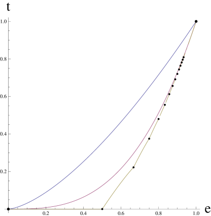
Figure 1: Region of attainable edge ($e$) and triangle ($t$) densities for graphons. The upper boundary is the curve $t=e^{3/2}$ and the lower boundary is a piecewise algebraic curve with infinitely many concave pieces; see [22]. The red curve is the Erdős-Renyi curve $t=e^{3}$.

The proof of Theorem 4.1 does not rely heavily on the definition of the edge-triangle model, except for the non-differentiability of $s(e,t)$ at $t=e^{3}$ and the structure of the maximizing graphons at the two extreme values of $\beta_{2}$. The following extension of this theorem may not come as a surprise.

Theorem 4.3.

Take $H_{1}$ a single edge and $H_{2}$ a different, arbitrary simple graph with chromatic number $\chi(H_{2})$ at least $3$. Consider the constrained repulsive $2$-parameter exponential random graph model where the probability measure $\mathbb{P}_{n}^{e,\beta_{2}}$ is given by

$$\mathbb{P}_{n}^{e,\beta_{2}}(G_{n})=\exp\left(n^{2}(\beta_{2}t(H_{2},G_{n})-\psi_{n}^{e,\beta_{2}})\right).$$ (4.9)

Let the edge density $e$ be fixed. Let the second parameter $\beta_{2}$ vary from $0$ to $-\infty$. Then $\psi^{e,\beta_{2}}$ loses its analyticity at at least one value of $\beta_{2}$.

Proof 4.4.

The proof of Theorem 4.1 carries over almost word-for-word when we incorporate the disordered Erdős-Rényi structure of the maximizing graphon at $\beta_{2}=0$, the non-differentiability of $s(e,t)$ for a general $H_{2}$ [20], and the emergent multipartite structure of the maximizing graphon as $\beta_{2}\rightarrow-\infty$ [8] [27].

Now that we know about the occurrence of a phase transition in the constrained repulsive exponential model, we probe deeper into this phenomenon and ask: how smooth is this transition? Theorem 4.5 shows what happens when the ideal edge density of the edge-triangle model is fixed at $1/2$ while the influence of the triangle densities is tuned through the parameter $\beta_{2}$.

Theorem 4.5.

Consider the constrained repulsive edge-triangle exponential random graph model as described at the beginning of Section 4. Fix $e=1/2$. Let $\beta_{2}$ vary from $0$ to $-\infty$. Then $\psi^{\frac{1}{2},\beta_{2}}$ is analytic everywhere except at a certain point $\beta_{2}^{c}$, where the derivative $\frac{\partial}{\partial\beta_{2}}\psi^{\frac{1}{2},\beta_{2}}$ displays jump discontinuity.

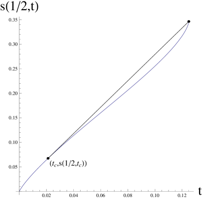
Figure 2: The graph of $s(1/2,t)$ below the ER line for the edge-triangle model (blue). The convex hull of the region below the graph is delimited by the black line segment and the portion of the graph to its left; this segment is the support line at the right endpoint $(t=1/8,s=\frac{\log 2}{2})$ of maximal slope $-\beta_{2}^{c}$. The other point at which the line segment meets the curve is the point $(t_{c},s(1/2,t_{c}))$.

Proof 4.6.

Setting $e=1/2$ in (4.2) gives

$$\psi^{\frac{1}{2},\beta_{2}}=\sup_{t}(\beta_{2}t+s(\frac{1}{2},t)).$$ (4.10)

Since $\beta_{2}\leq 0$, by the convexity of $I$, any maximizing graphon $h$ for (4.10) must satisfy $t(\tilde{h})\leq 1/8$, i.e., it must lie below the Erdős-Rényi curve $t=e^{3}$. Radin and Sadun [20] showed that on the line segment $e=\frac{1}{2}$ and $t\leq e^{3}$, the symmetric bipodal graphon

$$h(x,y)=\left\{\begin{array}[]{ll}\frac{1}{2}+\epsilon,&\hbox{if $x<\frac{1}{2}<y$ or $x>\frac{1}{2}>y$;}\\ \frac{1}{2}-\epsilon,&\hbox{if $x,y<\frac{1}{2}$ or $x,y>\frac{1}{2}$,}\\ \end{array}\right.$$ (4.11)

where $0\leq\epsilon=(\frac{1}{8}-t)^{\frac{1}{3}}\leq\frac{1}{2}$, maximizes $s(\frac{1}{2},t)$, and that every maximizing graphon is of the form $h_{\sigma}$ for some measure preserving bijection $\sigma$. Equivalently, the maximum value for (4.10) is achieved only at the reduced bipodal graphon $\tilde{h}$. See Figure 2 for the graph of $s(1/2,t)$.

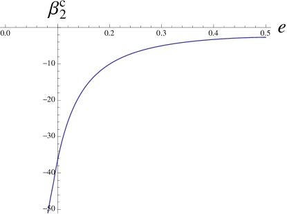
Figure 3: The (conjectural) graph of $\beta_{2}^{c}$ as a function of $e$ for the edge-triangle model, in the range $e\leq 1/2$. The computation is based on the conjecture that the maximizing graphons in this region are symmetric and bipodal, see [18].

Geometrically, the maximization problem in (4.10) involves finding the lowest half-plane with bounding line of slope $-\beta_{2}$ lying above the graph of $s(1/2,t)$. For $\beta_{2}>\beta_{2}^{c}$ the boundary of this half-plane passes only through the graph of $s(1/2,t)$ at the right endpoint $(\frac{1}{8},\frac{\log 2}{2})$. The critical value $\beta_{2}^{c}$ is defined (as in Figure 2) as the first slope at which this half-plane intersects the curve at a different point. We let $(t_{c},s(1/2,t_{c}))$ be this second point. At more negative values of $\beta_{2}$, the half-plane will hit the curve at points with $t$ values below $t_{c}$.

In particular this shows the non-analyticity of $\psi^{\frac{1}{2},\beta_{2}}$ as a function of $\beta_{2}$ at $\beta_{2}=\beta_{2}^{c}$. The analyticity of $\psi^{\frac{1}{2},\beta_{2}}$ elsewhere follows from concavity (and analyticity) of $s(1/2,t)$ below $t_{c}$. By Theorem 3.3, at $\beta_{2}=\beta_{2}^{c}$, the maximizing reduced graphon $\tilde{h}$ for (4.10) transitions from being Erdős-Rényi with edge formation probability $\frac{1}{2}$ to symmetric bipodal with $\epsilon_{c}=(\frac{1}{8}-t_{c})^{1/3}$. The jump discontinuity in the derivative follows when we realize that $\frac{\partial}{\partial\beta_{2}}\psi^{\frac{1}{2},\beta_{2}}=t(\tilde{h})$.

Numerical computations yield that $\beta_{2}^{c}$ is approximately $-2.7$ and $\epsilon_{c}$ is approximately $0.47$. By Theorem 3.3, this shows that as $\beta_{2}$ decreases from $0$ to $-\infty$, a typical graph $G_{n}$ drawn from the constrained repulsive edge-triangle model jumps from being Erdős-Rényi to almost complete bipartite, skipping a large portion of the $e=\frac{1}{2}$ line. This “jump behavior” (also called first-order phase transition) is intrinsically tied to the convexity of $s(e,t)$ just below the Erdős-Rényi curve $t=e^{3}$, thus we expect similar phase transition phenomena for general $e\neq\frac{1}{2}$ as well; see Figures 3, 4. However, unlike in the $e=\frac{1}{2}$ case, where the symmetry of $I$ (2.8) about $u=\frac{1}{2}$ contributes to a precise knowledge of the structure of the maximizing graphon, in general cases, there is only empirical evidence concerning the structure of the maximizing graphons. See also [8] for related results in the unconstrained repulsive edge-triangle model.

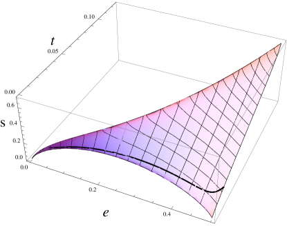
Figure 4: The (conjectural) graph of entropy $-I$ as a function of edge and triangle densities $e,t$ in the region $e\leq\frac{1}{2},t\leq e^{3}$. The critical curve (black) defines $t^{c}$ as a function of $e$. The computation is based on the conjecture that the maximizing graphons in this region are symmetric and bipodal, see [18].

5 Euler-Lagrange equations

We return to the constrained $2$-parameter family of exponential random graphs (4.9). For notational convenience and with some abuse of notation, denote by $T(h)=\sum_{i=1}^{2}\beta_{i}t(H_{i},h)$. As seen in Section 4, the “micro analysis” helps with the “macro analysis”. Explicitly, if we can find the maximizing graphon for $-I$ subject to two constraints $t(H_{1},\cdot)=t_{1}$ and $t(H_{2},\cdot)=t_{2}$, where $t_{1}$ and $t_{2}$ are arbitrary but fixed homomorphism densities, then we can find the maximizing graphon for $T-I$ subject to fewer or even no constraints. This in turn will aid us in understanding the limiting conditional probability distribution and the structure of a typical graph $G_{n}$ sampled from either the constrained or the unconstrained exponential model. In the unconstrained case, Chatterjee and Diaconis derived the Euler-Lagrange equation for the maximizing graphon $h$ for $T(h)-I(h)$ when the tuning parameters are arbitrary but fixed (Theorem 6.1 in [8]). When applied to the $2$-parameter model, they showed that $h$ must be bounded away from $0$ and $1$ and for almost all $(x,y)\in[0,1]^{2}$,

$$h(x,y)=\frac{e^{2\sum_{i=1}^{2}\beta_{i}\Delta_{H_{i}}h(x,y)}}{1+e^{2\sum_{i=1}^{2}\beta_{i}\Delta_{H_{i}}h(x,y)}},$$ (5.1)

where for a finite simple graph $H$ with vertex set $V(H)$ and edge set $E(H)$,

$$\Delta_{H}h(x,y)=\sum_{(r,s)\in E(H)}\Delta_{H,r,s}h(x,y),$$ (5.2)

and for each $(r,s)\in E(H)$ and each pair of points $x_{r},x_{s}\in[0,1]$,

$$\Delta_{H,r,s}h(x_{r},x_{s})=\\ \int_{[0,1]^{|}V(H)\texttt{\char 92\relax}\{r,s\}|}\prod_{(r^{\prime},s^{\prime})\in E(H):(r^{\prime},s^{\prime})\neq(r,s)}h(x_{r^{\prime}},x_{s^{\prime}})\prod_{v\in V(H):v\neq r,s}dx_{v}.$$ (5.3)

For example, in the edge-triangle model where $H_{1}$ is an edge and $H_{2}$ is a triangle, $\Delta_{H_{1}}h(x,y)\equiv 1$ and $\Delta_{H_{2}}h(x,y)=3\int_{0}^{1}h(x,z)h(y,z)dz$. In the constrained case, we could likewise derive the Euler-Lagrange equation by resorting to the method of Lagrange multipliers, which will turn the constrained maximization into an unconstrained one, but we provide an alternative bare-hands approach here. The following theorem may also be formulated in terms of reduced graphons.

Theorem 5.1.

Consider the constrained $2$-parameter exponential random graph model (4.9). Let $t_{1}$ and $t_{2}$ be arbitrary but fixed homomorphism densities. Suppose the graphon $h$ maximizes $-I(h)$ subject to $t(H_{1},h)=t_{1}$ and $t(H_{2},h)=t_{2}$. If $h$ is bounded away from $0$ and $1$, then there must exist constants $\beta_{1}$ and $\beta_{2}$ such that $h$ satisfies (5.1) for almost all $(x,y)\in[0,1]^{2}$.

Proof 5.2.

Graphons are bounded integrable functions on $[0,1]^{2}$ so they are continuous outside a set of arbitrarily small measure. Let $(x_{i},y_{i})$ for $i=1,2,3$ be three points of $[0,1]^{2}$. Inside a very small ball near $(x_{i},y_{i})$, write $h=h_{i}+\bar{h}$ where $h_{i}$ is the average of $h$ in that ball. We infinitesimally perturb the values of $h$ around $(x_{i},y_{i})$, sending $h_{i}\to h_{i}+dh_{i}$. Since $\bar{h}$ averages to $0$ and is pointwise small, in computing $t_{1},t_{2},$ and $-I$, terms involving $\bar{h}$ only contribute to second order and may be ignored in the computation below. Then $(t_{1},t_{2},-I)\rightarrow(t_{1},t_{2},-I)+(dt_{1},dt_{2},-dI)$ where

$$\left(\begin{array}[]{c}dt_{1}\\ dt_{2}\\ -dI\\ \end{array}\right)=\left(\begin{array}[]{cccc}\Delta_{H_{1}}h_{1}&\Delta_{H_{1}}h_{2}&\Delta_{H_{1}}h_{3}\\ \Delta_{H_{2}}h_{1}&\Delta_{H_{2}}h_{2}&\Delta_{H_{2}}h_{3}\\ \frac{1}{2}\log(\frac{1}{h_{1}}-1)&\frac{1}{2}\log(\frac{1}{h_{2}}-1)&\frac{1}{2}\log(\frac{1}{h_{3}}-1)\\ \end{array}\right)\left(\begin{array}[]{c}dh_{1}\\ dh_{2}\\ dh_{3}\\ \end{array}\right).$$ (5.4)

If the determinant of the above matrix is nonzero, then there is a nontrivial deformation $(dh_{1},dh_{2},dh_{3})$ which increases $-I$ while leaving $t_{1}$ and $t_{2}$ fixed. So the maximizing graphon $h$ must satisfy the condition that the determinant is zero. Recall that $H_{1}$ is a single edge and $\Delta_{H_{1}}h_{i}\equiv 1$. Without loss of generality we assume that $h_{1}\neq h_{2}$, since otherwise $h$ is a constant graphon and our claim trivially follows. Thus the first and third rows of the matrix are linearly independent and there must exist constants $\beta_{1}$ and $\beta_{2}$ such that

$$\Delta_{H_{2}}h_{i}=\beta_{1}+\frac{\beta_{2}}{2}\log(\frac{1}{h_{i}}-1).$$ (5.5)

Moreover, since $\beta_{1}$ and $\beta_{2}$ are determined by $h_{1}$ and $h_{2}$, we must have (5.5) for all points $(x_{3},y_{3})\in[0,1]^{2}$. We recognize this requirement is equivalent to (5.1).

Suppose we are looking for a graphon $h$ that maximizes $-I(h)$ subject to $t(H_{1},h)=t_{1}$ only. Then following the same “perturbation” idea, we should examine

$$\left(\begin{array}[]{c}dt_{1}\\ -dI\\ \end{array}\right)=\left(\begin{array}[]{cccc}\Delta_{H_{1}}h_{1}&\Delta_{H_{1}}h_{2}\\ \frac{1}{2}\log(\frac{1}{h_{1}}-1)&\frac{1}{2}\log(\frac{1}{h_{2}}-1)\\ \end{array}\right)\left(\begin{array}[]{c}dh_{1}\\ dh_{2}\\ \end{array}\right).$$ (5.6)

Since the determinant is zero, $h$ must be a constant. This is the same conclusion obtained by applying Jensen’s inequality to the convex function $I$. On the other hand, we may also consider maximizing $-I(h)$ subject to $k$ (instead of $2$) constraints $t(H_{i},h)=t_{i}$ for $i=1,\ldots,k$, in which case we would perturb the values of the graphon at $k+1$ points and form a $(k+1)\times(k+1)$ matrix.

Richard Kenyon’s research was partially supported by NSF grant DMS-1208191 and a Simons Investigator award. Mei Yin’s research was partially supported by NSF grant DMS-1308333. They thank Charles Radin, Kui Ren, and Lorenzo Sadun for helpful conversations.

References

- [1] Aristoff, D, Radin, C.: Emergent structures in large networks. J. Appl. Prob. 50, 883-888 (2013)
- [2] Aldous, D.: Representations for partially exchangeable arrays of random variables. J. Multivariate Anal. 11, 581-598 (1981)
- [3] Bollobás, B.: Random Graphs, Volume 73 of Cambridge Studies in Advanced Mathematics. 2nd ed. Cambridge University Press, Cambridge (2001)
- [4] Borgs, C., Chayes, J.T., Cohn, H., Zhao, Y: An theory of sparse graph convergence I. Limits, sparse random graph models, and power law distributions. arXiv: 1401.2906 (2014)
- [5] Borgs, C., Chayes, J., Lovász, L., Sós, V.T., Vesztergombi, K.: Counting graph homomorphisms. In: Klazar, M., Kratochvil, J., Loebl, M., Thomas, R., Valtr, P. (eds.) Topics in Discrete Mathematics, Volume 26, pp. 315-371. Springer, Berlin (2006)
- [6] Borgs, C., Chayes, J.T., Lovász, L., Sós, V.T., Vesztergombi, K.: Convergent sequences of dense graphs I. Subgraph frequencies, metric properties and testing. Adv. Math. 219, 1801-1851 (2008)
- [7] Borgs, C., Chayes, J.T., Lovász, L., Sós, V.T., Vesztergombi, K.: Convergent sequences of dense graphs II. Multiway cuts and statistical physics. Ann. of Math. 176, 151-219 (2012)
- [8] Chatterjee, S., Diaconis, P.: Estimating and understanding exponential random graph models. Ann. Statist. 41, 2428-2461 (2013)
- [9] Chatterjee, S., Diaconis, P., Sly, A.: Random graphs with a given degree sequence. Ann. Appl. Prob. 21, 1400-1435 (2011)
- [10] Chatterjee, S., Varadhan, S.R.S.: The large deviation principle for the Erdős-Rényi random graph. European J. Combin. 32, 1000-1017 (2011)
- [11] Frank, O., Strauss, D.: Markov graphs. J. Amer. Statist. Assoc. 81, 832-842 (1986)
- [12] Häggström, O., Jonasson, J.: Phase transition in the random triangle model. J. Appl. Probab. 36, 1101-1115 (1999)
- [13] Hoover, D.: Row-column exchangeability and a generalized model for probability. In: Koch, G., Spizzichino, F. (eds.) Exchangeability in Probability and Statistics, pp. 281-291. North-Holland, Amsterdam (1982)
- [14] Lovász, L.: Large Networks and Graph Limits. American Mathematical Society, Providence (2012)
- [15] Lovász, L., Szegedy B.: Limits of dense graph sequences. J. Combin. Theory Ser. B 96, 933-957 (2006)
- [16] Lubetzky, E., Zhao, Y.: On the variational problem for upper tails in sparse random graphs. arXiv: 1402.6011 (2014)
- [17] Newman, M.: Networks: An Introduction. Oxford University Press, New York (2010)
- [18] Radin, C., Ren, K., Sadun, L.: The asymptotics of large constrained graphs. arXiv: 1401.1170 (2014)
- [19] Radin, C., Sadun, L.: Phase transitions in a complex network. J. Phys. A 46, 305002 (2013)
- [20] Radin, C., Sadun, L.: Singularities in the entropy of asymptotically large simple graphs. arXiv: 1302.3531 (2013)
- [21] Radin, C., Yin, M.: Phase transitions in exponential random graphs. Ann. Appl. Probab. 23, 2458-2471 (2013)
- [22] Razborov, A.: On the minimal density of triangles in graphs. Combin. Probab. Comput. 17, 603-618 (2008)
- [23] Touchette, H., Ellis, R.S., Turkington, B.: An introduction to the thermodynamic and macrostate levels of nonequivalent ensembles. Physica A 340, 138-146 (2004)
-
[24]
van der Hofstad, R.: Random Graphs and Complex Networks.
http://www.win.tue.nl/rhofstad/NotesRGCN.pdf (2014) - [25] Wasserman, S., Faust, K.: Social Network Analysis: Methods and Applications. Cambridge University Press, Cambridge (2010)
- [26] Yin, M.: Critical phenomena in exponential random graphs. J. Stat. Phys. 153, 1008-1021 (2013)
- [27] Yin, M., Rinaldo, A., Fadnavis, S.: Asymptotic quantization of exponential random graphs. arXiv: 1311.1738 (2013)