Optimal control of storage incorporating market impact
and with energy applications

Abstract

Large scale electricity storage is set to play an increasingly important role in the management of future energy networks. A major aspect of the economics of such projects is captured in arbitrage, i.e. buying electricity when it is cheap and selling it when it is expensive. We consider a mathematical model which may account for nonlinear—and possibly stochastically evolving—cost functions, market impact, input and output rate constraints and both time-dependent and time-independent inefficiencies or losses in the storage process. Our main concern is to develop the associated strong Lagrangian theory. The Lagrange multipliers associated with the capacity constraints in particular have important economic interpretations with regard to the dimensioning of storage—both with respect to its capacity and its rate constraints—and prove key to the efficient control of a store. We also develop an algorithm which determines, sequentially in time, both these Lagrange multipliers and the optimal control. This algorithm further identifies, for each point in time, a time horizon beyond which it is not necessary to look in order to identify the optimal control at that point; this horizon is furthermore the shortest such. The algorithm is thus particularly suitable for the management of storage over extended periods of time. We give examples related to the management of real-world systems. Finally we consider a pragmatic approach to the real-time management of storage in a stochastic cost environment, which is computationally feasible, optimal under certain ideal conditions, and which may in general be expected to perform close to optimally. Our results are formulated in a general setting which permits their application to other energy management problems, and to other commodity storage problems.

1 Introduction

How should one optimally control an energy store which is used to make money by buying electricity when it is cheap, and selling it when it is expensive? While in its simplest form this is a classical mathematical problem (see [10] and, for early dynamic programming approaches, [6] and [13]) we are interested in the problem where the store has both finite capacity and rate constraints, and where we allow that the activities of the store are of a sufficient magnitude as to impact upon prices in the market in which it operates. The underlying mathematics thus required has various novel features and needs to be carefully formulated so as to properly account for physical characteristics of different storage technologies and to deal with inherent nonlinearities which occur when prices are impacted by the store’s behaviour.

A closely related application is to the management of demand in such systems, where the ability to contract with consumers to postpone demand may be regarded as negative storage. For some recent discussion and work on these applications see, for example, [1, 17, 19, 21, 23, 28, 30] and the references therein; for work on the optimal placement of storage within a network, see [26, 27]. These works are concerned, as here, with the mathematics of storage for arbitrage, i.e. taking advantage of—and hence assisting in smoothing—-price fluctuations over time. This mathematics is of course also quite generally applicable to the use of storage in other markets. (For the mathematics of other uses of storage in energy systems—notably for buffering against uncertainty—see, for example, [3, 4, 5, 15, 18, 20, 30].)

We think of the available storage as a single store. Its value is equal to the profit which can be made by a notional store “owner” buying and selling as above. Our particular interest is in the case where the activities of the store are sufficiently significant as to have a market impact (the store becomes a “price-maker”). In this case the store owner sees nonlinear cost functions as, at any time, the marginal costs of buying or returns from selling vary with the amount being bought or sold. In the case where the system or societal value of the store is required, this may be similarly calculated by adjusting the notional buying and selling prices so that the store “owner” is required to bear also the external costs of the store’s activities (see below for further discussion of this).

The nonlinearity of the cost functions means that the linear programming techniques which might otherwise be used in the solution of this problem are not generally available. (However, see Section 2 for some further discussion and references for the case where linear programming techniques may be used.) Neither are dynamic programming techniques—deterministic or stochastic (see, for example, [7, 8])—always tractable in practice. The reason for the latter is that optimization is typically over extended periods of time, during which the costs involved usually vary with time in an irregular manner. The computational complexity of a dynamic programming approach may therefore be unduly burdensome and is almost certainly so in a stochastic environment. Further, in the presence of temporal heterogeneity dynamic programming approaches may fail to provide necessary insights—for example, concerning the time horizons necessary for optimal decision making, or sensitivities with respect to local cost variations.

In the present paper we develop an approach based on the use of strong Lagrangian techniques (convex optimization theory) which naturally accommodates nonlinear cost functions, input and output rate constraints, and temporal heterogeneity, and for which the associated Lagrange multipliers provide the information necessary for the correct dimensioning of storage with respect to both capacity and rate constraints, and for the assessment of the economics of storage in networks. The strong Lagrangian approach also enables the development of an algorithm for the solution of the problem which is efficient in the sense that the decisions to be made at each point in time typically depend only on a very short future horizon—which is identifiable, but not determined in advance. The length of this horizon (the definition of which we make precise in Section 4) depends on the parameters of the store and is of the same order as that of the shortest period of time over which prices fluctuate significantly; this is important when we may wish to optimally manage a store over a very much longer, or perhaps indefinite, period of time. Our approach also allows us to account for differences in buying and selling prices and for both time-dependent and time-independent inefficiencies in the storage process.

Initially we work in a deterministic setting in which we assume that all relevant buying and selling prices are known in advance. For many applications this is reasonable: as indicated above (and in the realistic examples of Section 6) the time horizon required for optimal decision making may be short. However, elsewhere there is a need to take account of stochastic variation, and in Section 7 we consider prices which evolve stochastically. We show that in a somewhat idealised stochastic setting—in which uncertainty evolves backwards in time as a martingale—the optimal control is simply to replace future costs by their expected values and to proceed as in the deterministic case. We argue also that that this approach should continue to work well in a more general stochastic setting when combined with the possibility of re-optimisation at each time step.

In Section 2 we formally define the relevant mathematical problem, while in Section 3 we use strong Lagrangian theory to characterise mathematically its optimal solution. We use this theory in Section 4 to develop the algorithm for the solution referred to above and to characterise the evolving time horizon required for decision making in a dynamic environment. In Section 5 we show how the value of the store changes with respect to variation in its characteristic parameters. Section 6 considers examples based on real data for UK electricity prices. Section 7 studies models in which the cost functions vary stochastically as described above, and proposes an approach which we believe is as realistic as is practicable for many applications.

2 Problem formulation

We work in discrete time, which we take to be integer. We assume that the store has total capacity of $E$ (which, in the context of an energy system, would be total energy which could be stored) and input and output rate constraints of $P_{i}$ and $P_{o}$ respectively (which, for an energy system, would be in units of power). We consider two types of (in)efficiency associated with the store. The first of these (and usually much the more significant in practice) is a time-independent efficiency $\eta$ which may be defined as the fraction of energy bought which is available to sell. This may be incorporated directly into the cost functions $C_{t}$, by suitably rescaling selling and buying prices. The second type of (in)efficiency may be regarded as leakage over time, and is modelled by assuming that at each successive time instant there is lost a fraction $1-\rho$ of whatever is in the store at that time. We remark that it would also be possible to assume, without loss of generality, that there was no leakage, i.e. that $\rho=1$; this could be achieved by adjusting by a factor $\rho^{t}$ the units of measurement of the volume in storage at each time $t$ and suitably redefining cost functions and constraints; however, there is very little effort saved by introducing this additional level of abstraction, and so we in general avoid doing so.

Let $X=\{x:-P_{o}\leq x\leq P_{i}\}$. Both buying and selling prices at time $t$ may conveniently be represented by a cost function $C_{t}$, which we assume to be convex, and is such that $C_{t}(x)$ is the cost at time $t$ of increasing the level of the store contents (after any leakage—see below) by $x$, positive or negative. Typically—in a conventional store and with positive prices—we have that each function $C_{t}$ is increasing and that $C_{t}(0)=0$; then, for positive $x$, $C_{t}(x)$ is the cost of buying $x$ units (for example of energy) and, for negative $x$, $C_{t}(x)$ is the negative of the reward for selling $-x$ units; however, for some applications (see below), the interpretation of the functions $C_{t}$ may vary slightly from this, and only the convexity condition on these functions is required. This convexity assumption corresponds, for each time $t$, to an increasing cost to the store of buying each additional unit, a decreasing revenue obtained for selling each additional unit, and every unit buying price being at least as great as every unit selling price. Note that incorporating the time-independent (or “round-trip”) efficiency $\eta$ into the cost functions $C_{t}$, as discussed above, automatically preserves convexity whenever these cost functions are increasing. For a discussion of non-convex cost functions, see for example [14].

We are not concerned here to discuss the market derivation of the functions $C_{t}$, for a discussion of which see, for example, [11].

As indicated above, if the problem is to determine the value of the store to the entire system in which it operates, or to society, then these prices are taken to be those appropriate to the system or to be societal costs. Thus, for example, for $x$ positive, $C_{t}(x)$ may be the price paid by the store at time $t$ for $x$ units of, for example, energy plus the increased cost paid by other energy users at that time as a result of the store’s purchase increasing market prices—again see [11] for a detailed explanation of how the current model may be used in this context.

Figure 1 thus illustrates a typical cost function $C_{t}$. While the function $C_{t}$ may be formally regarded as defined over the whole real line, the rate constraints means that for the purposes of the present problem its domain is effectively restricted to the set $X$ defined above. (We shall later wish to consider the effect of varying the rate constraints.)

Figure 1: Illustrative cost function $C_{t}$. The domain of the function is effectively restricted to the set $X=\{x:-P_{o}\leq x\leq P_{i}\}$.

A special case is that of a “small” store, whose operations do not influence the market (the store is a “price-taker” rather than a “price-maker”), and which at time $t$ buys and sells at given prices per unit of $c^{(b)}_{t}$ and $c^{(s)}_{t}$ respectively, where we assume that $c^{(b)}_{t}\geq c^{(s)}_{t}$. Here the function $C_{t}$ is given by

$$C_{t}(x)=\begin{cases}c^{(b)}_{t}x&\quad\text{if $x\geq 0$}\\ c^{(s)}_{t}x&\quad\text{if $x<0$}.\end{cases}$$ (1)

Finally, we assume for the moment that all prices are known in advance, so that the problem of controlling the store is deterministic. We consider a realistic stochastic model in Section 7.

Denote the successive levels of the store by a vector $S=(S_{0},\dots,S_{T})$ where $S_{t}$ is the level of the store at each successive time $t$. Define also the vector $x(S)=(x_{1}(S),\dots,x_{T}(S))$ by $x_{t}(S)=S_{t}-\rho S_{t-1}$ for each $t\geq 1$. Here $\rho$ is the leakage measure defined above, so that $x_{t}(S)$ represents the addition to the store at time $t$. It is convenient to assume that both the initial level $S_{0}$ and the final level $S_{T}$ of the store are fixed in advance at $S_{0}=S^{*}_{0}$ and $S_{T}=S^{*}_{T}$. (If the final level $S_{T}$ is not fixed and the cost function $C_{T}$ is strictly increasing, then, for an optimal control, we may take $S_{T}$ to be minimised—so that finally as much as possible of the contents of the store are sold; however, we might, for example, wish to require $S^{*}_{T}=S^{*}_{0}$ in order to solve a problem in which the cost functions varied cyclically.)

The problem thus becomes:

• (given the convex functions $C_{t}$) choose $S$ so as to minimise

  $$G(S):=\sum_{t=1}^{T}C_{t}(x_{t}(S))$$ (2)

  subject to the capacity constraints

  $$S_{0}=S^{*}_{0},\qquad S_{T}=S^{*}_{T},\qquad 0\leq S_{t}\leq E,\quad 1\leq t\leq T-1.$$ (3)

  and the rate constraints

  $$x_{t}(S)\in X,\qquad 1\leq t\leq T.$$ (4)

We shall say that a vector $S$ is feasible for the problem $\mathbf{P}$ if it satisfies both the capacity constraints (3) and the rate constraints (4). We shall assume that $S^{*}_{0}$ and $S^{*}_{T}$ are sufficiently close that it is possible to change the level of the store from $S^{*}_{0}$ to $S^{*}_{T}$ between times $0$ and $T$, i.e. that the set of feasible vectors $S$ is nonempty. Note that this set is then closed and convex and that the function $G$ defined by (2) is convex, and strictly so when the functions $C_{t}$ are strictly convex. Hence a solution to the problem $\mathbf{P}$ always exists, and is unique when the functions $C_{t}$ are strictly convex.

In the case where the cost functions $C_{t}$ are linear, or piecewise linear, as in the “small store” case given by (1), the problem $\mathbf{P}$ may be reformulated as a linear programming problem, and solved by, for example, the use of the minimum cost circulation algorithm (see, for example, [9, 2]). Our aim in the present paper is to deal with the general case, to develop the related Lagrangian theory together with an algorithm which identifies both problem solution and associated Lagrange multipliers, and to use this algorithm to show that the optimal choice of $S_{t}$ at each time $t$ depends only on a typically very short time horizon, thus providing an efficient approach to the solution of the problem (particularly the real-time management of the store within applications) over long time periods.

Finally, we note that the mathematical problem formulated in this section is applicable to physical problems—in energy management and elsewhere—other than those of conventional storage. One such is the management of “one-sided” storage, such as hydroelectric power, in which inputs are predetermined and (we assume here) known and the only control is over the output at each successive time $t$. Here the control remains the sequence $S$ of successive levels of the store, and, for each $t$, the function $C_{t}$ is such that $C_{t}(x_{t}(S))$ remains the cost of the “change” $x_{t}(S)$ as defined earlier. It may not here be natural to have $C_{t}(0)=0$, and we may wish to allow the space $X$ of feasible values of $x_{t}(S)$ to depend on the time $t$—something which causes no additional complications.

A further possible application might be to the buffering of demand, which, as remarked earlier, may be regarded as negative storage, $S_{t}$ now being the amount of demand “postponed” at each successive time $t$. The cost functions $C_{t}$ would represent the costs of such postponement. However, to be realistic such costs would probably also need to reflect the durations of such postponements.

3 Lagrangian formulation and characterisation of solution

We develop the strong Lagrangian theory [9, 29] associated with the problem $\mathbf{P}$ defined above. Theorem 1 gives sufficient conditions for a value $S^{*}$ of $S$ to solve the problem, while Theorem 2 guarantees the existence of such a value of $S^{*}$, together with the associated vector (cumulative Lagrange multiplier) $\mu^{*}$ defined there.

Theorem 1.

Suppose that there exists a vector $\mu^{*}=(\mu^{*}_{1},\dots,\mu^{*}_{T})$ and a value $S^{*}=(S^{*}_{0},\dots,S^{*}_{T})$ of $S$ such that

1. $S^{*}$ is feasible for the stated problem,

2. for each $t$ with $1\leq t\leq T$, $x_{t}(S^{*})$ minimises $C_{t}(x)-\mu^{*}_{t}x$ in $x\in X$,

3. the pair $(S^{*},\mu^{*})$ satisfies the complementary slackness conditions, for $1\leq t\leq T-1$,

   $$\begin{cases}\rho\mu^{*}_{t+1}=\mu^{*}_{t}&\quad\text{if $0<S^{*}_{t}<E$,}\\ \rho\mu^{*}_{t+1}\leq\mu^{*}_{t}&\quad\text{if $S^{*}_{t}=0$,}\\ \rho\mu^{*}_{t+1}\geq\mu^{*}_{t}&\quad\text{if $S^{*}_{t}=E$.}\end{cases}$$ (5)

Then $S^{*}$ solves the stated problem $\mathbf{P}$.

Proof.

Let $S$ be any vector which is feasible for the problem (with $S_{0}=S^{*}_{0}$ and $S_{T}=S^{*}_{T}$). Then, from the condition (ii),

$$\sum_{t=1}^{T}\left[C_{t}(x_{t}(S^{*}))-\mu^{*}_{t}x_{t}(S^{*})\right]\leq\sum_{t=1}^{T}\left[C_{t}(x_{t}(S))-\mu^{*}_{t}x_{t}(S)\right].$$

Rearranging and recalling that $S$ and $S^{*}$ agree at $0$ and at $T$, we have

$$\sum_{t=1}^{T}C_{t}(x_{t}(S^{*}))-\sum_{t=1}^{T}C_{t}(x_{t}(S)) \leq\sum_{t=1}^{T}\mu^{*}_{t}(S^{*}_{t}-\rho S^{*}_{t-1}-S_{t}+\rho S_{t-1})$$

$$=\sum_{t=1}^{T-1}(S^{*}_{t}-S_{t})(\mu^{*}_{t}-\rho\mu^{*}_{t+1})$$

$$\leq 0,$$

by the condition (iii), so that the result follows. ∎

Remark 1.

Note that when the functions $C_{t}$ are increasing the vector $\mu^{*}$ of Theorem 1 may be taken to be nonnegative, i.e. to have nonnegative components: if $\mu^{*}$ does not satisfy this condition then its negative components may all be increased to $0$ and the pair $(S^{*},\,\mu^{*})$ will continue to satisfy the conditions of the theorem.

The vector $\mu^{*}$ is a cumulative form of the vector of Lagrange multipliers associated with the capacity constraints (3) (see the proof of Theorem 2 below). It has the interpretation that, for each $t$, the quantity $\mu^{*}_{t}$ may be regarded as a notional reference value per unit volume in storage at that time. Thus, in the condition (ii) of the theorem, $C_{t}(x)$ is the cost at time $t$ of increasing the level of the store by $x$ (again positive or negative) and $\mu^{*}_{t}x$ may be regarded as a current offsetting measure of value added to the store; the quantity $C_{t}(x)-\mu^{*}_{t}x$ is thus to be minimised in $x\in X$. The relations (5) of condition (iii) of the theorem are then such that, were they to be violated, $x_{t}$ and $x_{t+1}$ could in general be adjusted so as to leave unchanged the level of the store at the end of time $t+1$ while reducing the overall cost of operating the store throughout the period consisting of the times $t$ and $t+1$.

Note also that, in the condition (ii) of Theorem 1, the minimisation takes place without reference to the capacity constraints (as is appropriate given the above Lagrangian interpretation of $\mu^{*}$). However, the minimisation of that condition is required to respect the rate constraints $x\in X$—for which no Lagrange multiplier is introduced at this stage (but see Section 5). The reason for the apparent asymmetry of treatment of the two constraint types is that it is only the capacity constraints which introduce complexity into the optimisation problem, by introducing interactions between the amounts which may be bought and sold at different times. The rate constraints could, if we wished, be dropped from the formal statement of the problem by suitably modifying the cost functions so that the violation of these constraints was simply prohibitively expensive.

Before considering Theorem 2, which guarantees the existence of the pair $(S^{*},\mu^{*})$, we give a couple of simple examples, in each of which the reference vector $\mu^{*}$ is identified. Theorem 1 is not, however, needed for the solution of the first, very simple, example. It is needed in the second example only in the case where the store is sufficiently large as to have market impact (i.e. be a price-maker).

Example 1.

As a simple (toy) example, suppose that $T=2$ and that the cost functions $C_{t}$, $t=1,2$, in addition to being increasing and convex, are differentiable (with necessarily continuous first derivatives); however, as an exception and in order to allow for a distinction between buying and selling prices we allow a difference between the left and right derivatives of the functions $C_{t}$ at $0$, denoting these one-sided derivatives by $C^{\prime}_{t}(0-)$ and $C^{\prime}_{t}(0+)$ respectively (with, necessarily, $C^{\prime}_{t}(0-)\leq C^{\prime}_{t}(0+)$ for $t=1,2$). We suppose additionally, and again for simplicity, that the input and output rate constraints are equal, setting $P_{i}=P_{o}=P$, and that there is no leakage (i.e. $\rho=1$). Finally we suppose $S^{*}_{0}=S^{*}_{2}=0$ so that the store starts empty and is required to finish empty. Thus the only possible control of the store lies in the choice of the amount $x\geq 0$ which is bought at time $1$ and sold again at time $2$.

For this example, the optimal policy is of course easily determined. Our concern is merely to identify, in this very simple case, the vector $\mu^{*}$ of Theorem 1. This vector plays a crucial rôle in more complex optimization over longer time periods. We consider the three possible cases.

1. If $C^{\prime}_{1}(0+)\geq C^{\prime}_{2}(0-)$ then clearly the optimal policy is buy and sell nothing and we take $x=0$. For the vector $\mu^{*}$ of Theorem 1 we may take $\mu^{*}_{1}=C_{1}^{\prime}(0+)$ and $\mu^{*}_{2}=C_{2}^{\prime}(0-)$.

2. If $C^{\prime}_{1}(0+)<C^{\prime}_{2}(0-)$ and there exists $x$ such that both $0\leq x\leq\min(E,\,P)$ and $C^{\prime}_{1}(x)=C^{\prime}_{2}(-x)$, then this choice of $x$ is again clearly optimal. The vector $\mu^{*}$ is given (uniquely) by $\mu^{*}_{1}=\mu^{*}_{2}=C^{\prime}_{1}(x)$.

3. Finally, if $C^{\prime}_{1}(x)<C^{\prime}_{2}(-x)$ for all $x$ such that $0\leq x\leq\min(E,\,P)$, then the optimal choice of $x$ is given by $x=\min(E,\,P)$. In the case where $P\leq E$ we require $C^{\prime}_{1}(P)\leq\mu^{*}_{1}=\mu^{*}_{2}\leq C^{\prime}_{2}(-P)$, while in the case where $E<P$ we require $C^{\prime}_{1}(E)=\mu^{*}_{1}\leq\mu^{*}_{2}=C^{\prime}_{2}(-E)$.

Note that the actual solution to this very simple problem depends on $E$ and $P$ only through $\min(E,\,P)$. However, as previously observed, $\mu^{*}$ plays an asymmetric rôle with respect to capacity and rate constraints and thus formally differs in the case (iii) according to which of $E$ or $P$ is the greater.

Example 2.

Periodic costs. As a second simple example, we suppose that the cost functions vary over time in a manner which is completely periodic. To begin with, we consider the “small store”, or price-taker, case in which the cost functions $C_{t}$ are given by (1) (with $c^{(b)}_{t}\geq c^{(s)}_{t}$ for all $t$). We suppose that the periodic behaviour is such that, at some time $t_{1}$ in a cycle, both $c^{(b)}_{t_{1}}$ and $c^{(s)}_{t_{1}}$ are simultaneously at a minimum; the unit costs $c^{(b)}_{t}$ and $c^{(s)}_{t}$ then increase monotonically up to a time $t_{2}>t_{1}$ where they are simultaneously at a maximum, before decreasing monotonically again to the same minimum value as previously at further time $t_{3}>t_{2}$; this pattern is then repeated indefinitely with period $t_{3}-t_{1}$. We suppose also that the minimum value of the unit buy costs $c^{(b)}_{t}$ is less than the maximum value of the unit sell costs $c^{(s)}_{t}$ (otherwise the store remains unused). We again assume, for simplicity, that there is no leakage (i.e. $\rho=1$), that $P_{i}=P_{o}=P$ and that time is sufficiently finely discretised that $E/P$ (the minimum time in which the store may completely empty or fill) may be taken to be integer. The optimal control policy depends (up to a multiplicative constant) on $E$ and $P$ only through the ratio $E/P$; hence, without loss of generality, we assume $P=1$.

The simplicity of this example is such that the optimal control of the store is again immediately clear: for all $E$ there exist reference costs $\mu^{(b)}\leq\mu^{(s)}$ such that the store buys the maximum value of one unit at those times such that $c^{(b)}_{t}<\mu^{(b)}$ and sells the maximum value of one unit at those times such that $c^{(s)}_{t}>\mu^{(s)}$; for $E$ sufficiently small we may take $\mu^{(b)}<\mu^{(s)}$ and the store completely empties and fills on each cycle; however, as $E$ increases it reaches a value at which the reference costs $\mu^{(b)}$ and $\mu^{(s)}$ equalise, and for this and larger values of $E$ the capacity constraint is no longer binding.

As in the case of the previous example, this “small store” problem is too simple for its solution to require the use of the reference vector $\mu^{*}$ of Theorem 1 (but see below for where it is needed). We note, however, that this vector may be given by $\mu^{*}_{t}=\mu^{(b)}$ at those times $t$ at which the store is buying, and by $\mu^{*}_{t}=\mu^{(s)}$ at those times $t$ at which it is selling; at other times (at each of which the store will either be completely full or completely empty) $\mu^{*}_{t}$ is merely required to satisfy the condition (iii) of Theorem 1 together with the condition $c^{(s)}_{t}\leq\mu^{*}_{t}\leq c^{(b)}_{t}$ (so that the condition (ii) of Theorem 1 is satisfied).

We also comment briefly on the effect of varying the frequency of the cost variation. If, in what should strictly be a continuous-time setting, this frequency is increased by a factor $\alpha$ with the rate constraint $P$ being similarly increased by the same factor, then this corresponds to a simple time speed-up, with the store’s revenue per unit time also being increased by the factor $\alpha$. However, suppose instead that while the frequency of the cost variation is increased by the factor $\alpha$, the rate constraint $P$ is held constant at its original value and that the capacity constraint $E$ is replaced by $E/\alpha$. It then follows, from the earlier observation that the optimal control depends on $E$ and $P$ only through their ratio, that the optimal control is here a rescaled version of the original and that the store’s revenue per unit time remains unchanged from the original. Thus we have the well-known result that more frequent cost variation enables the same revenue to be obtained with a smaller store capacity.

When we consider the general case in which the store is a price-maker, and in which the cost functions $C_{t}$ have the same general periodicity over time, but no longer have the simple structure given by (1), then the store may fill and empty over periods of time which are longer than the minimum necessary, so as to avoid the higher costs or penalties of buying or selling too much at once. The reference vector $\mu^{*}$ of Theorem 1 then becomes essential in deciding the correct volume of each transaction.

Theorem 1 does not require the convexity of the cost functions $C_{t}$ of the problem $\mathbf{P}$ defined in Section 2. This condition is, however, required to ensure the existence of the vector $\mu^{*}$ of that theorem, as is given by Theorem 2 below. The latter theorem identifies $\mu^{*}$ as essentially a cumulative Lagrange multiplier for capacity constraint variation. It is a further application of arguments to be found in strong Lagrangian theory (again see [29]).

We have already observed that, under strict convexity of the cost functions $C_{t}$, the solution $S^{*}$ to the problem $\mathbf{P}$ is unique. However, we further remark that even this condition is insufficient to guarantee uniqueness of $\mu^{*}$ as above. We address this issue in Section 5, where we assume sufficient differentiability conditions on the cost functions $C_{t}$ as to ensure uniqueness of $\mu^{*}$ and to derive sensitivity results for variation of the minimised cost function of $\mathbf{P}$ with respect to both its capacity and rate constraints.

Prior to Theorem 2 it is convenient to introduce the more general problem $\mathbf{P}(a,\,b)$ in which $S_{0}$ is kept fixed at the value $S^{*}_{0}$ of interest above, but in which $S_{1},\dots,S_{T}$ are allowed to vary between quite general upper and lower bounds:

• minimise $\sum_{t=1}^{T}C_{t}(x_{t}(S))$ over all $S=(S_{0},\dots,S_{T})$ with $S_{0}=S^{*}_{0}$ and subject to the further constraints

  $$a_{t}\leq S_{t}\leq b_{t},\qquad 1\leq t\leq T,$$ (6)

  and $x_{t}(S)\in X$ for $1\leq t\leq T$, where $a=(a_{1},\dots,a_{T})$ and $b=(b_{1},\dots,b_{T})$ are such that $a_{t}\leq b_{t}$ for all $t$.

Note that the convexity of the functions $C_{t}$ guarantees their continuity, and, since for each $a$, $b$ as above the space of allowed values of $S$ is compact, a solution $S^{*}(a,\,b)$ to the problem $\mathbf{P}(a,\,b)$ always exists. Let $V(a,\,b)$ be the corresponding minimised value of the objective function, i.e. $V(a,\,b)=\sum_{t=1}^{T}C_{t}(x_{t}(S^{*}(a,\,b)))$. Then $V(a,\,b)$ is itself convex in $a$ and $b$. (To see this, consider, for example, any convex combination $(\bar{a},\bar{b})=(\lambda a_{1}+(1-\lambda)a_{2},\lambda b_{1}+(1-\lambda)b_{2})$ of any two values $(a_{1},b_{1})$ and $(a_{2},b_{2})$ of the pair $(a,b)$, where $0\leq\lambda\leq 1$; the linearity of the constraints (3) and (4) implies that the vector $\bar{S}=\lambda S^{*}(a_{1},b_{1})+(1-\lambda)S^{*}(a_{2},b_{2})$ is feasible for the problem $\mathbf{P}(\bar{a},\,\bar{b})$; hence

$$V(\bar{a},\bar{b}) \leq\sum_{t=1}^{T}C_{t}(x_{t}(\bar{S}))$$

$$=\sum_{t=1}^{T}C_{t}(\lambda x_{t}(S^{*}(a_{1},b_{1}))+(1-\lambda)x_{t}(S^{*}(a_{2},b_{2})))$$

$$\leq\lambda\sum_{t=1}^{T}C_{t}(x_{t}(S^{*}(a_{1},b_{1})))+(1-\lambda)\sum_{t=1}^{T}C_{t}(x_{t}(S^{*}(a_{2},b_{2})))$$

$$=\lambda V(a_{1},b_{1})+(1-\lambda)V(a_{2},b_{2}),$$

where the second inequality above follows from the convexity of the functions $C_{t}$.) Define also $a^{*}$ and $b^{*}$ to be the values of $a$ and $b$ corresponding to our particular problem $\mathbf{P}$ of interest, i.e. $a^{*}_{t}=0$ and $b^{*}_{t}=E$ for $1\leq t\leq T-1$, and $a^{*}_{T}=b^{*}_{T}=S^{*}_{T}$. Further, let $S^{*}=(S^{*}_{0},\dots,S^{*}_{T})=S^{*}(a^{*},\,b^{*})$ denote the solution to this problem.

Theorem 2.

Under the given convexity condition on the cost functions $C_{t}$, there always exists a pair $(S^{*},\mu^{*})$ which solves the problem $\mathbf{P}$ as in Theorem 1.

Proof.

Consider the more general problem $\mathbf{P}(a,\,b)$ defined above. Introduce slack (or surplus) variables $z=(z_{1},\dots,z_{t})$ and $w=(w_{1},\dots,w_{t})$ and rewrite this problem as:

• minimise $\sum_{t=1}^{T}C_{t}(x_{t}(S))$ over all $S=(S_{0},\dots,S_{T})$ with $S_{0}=S^{*}_{0}$, all $z\geq 0$, all $w\geq 0$, and subject to the further constraints

  $$S_{t}-z_{t} =a_{t},\qquad 1\leq t\leq T,$$ (7)

  $$S_{t}+w_{t} =b_{t},\qquad 1\leq t\leq T,$$ (8)

  and, again, $x_{t}(S)\in X$ for $1\leq t\leq T$.

Since, as already observed, the function $V(a,\,b)$ is itself convex in $a$ and $b$, it follows by the supporting hyperplane theorem (see [9] or [29]), that there exist vectors (Lagrange multipliers) $\alpha^{*}=(\alpha^{*}_{1},\dots,\alpha^{*}_{T})$ and $\beta^{*}=(\beta^{*}_{1},\dots,\beta^{*}_{T})$ such that

$$V(a,\,b)\geq V(a^{*},\,b^{*})+\sum_{t=1}^{T}\alpha^{*}_{t}(a_{t}-a^{*}_{t})+\sum_{t=1}^{T}\beta^{*}_{t}(b_{t}-b^{*}_{t})\qquad\text{for all $a$, $b$}.$$ (9)

Thus also, for all $S$ with $S_{0}=S^{*}_{0}$ and such that $x_{t}(S)\in X$ for $1\leq t\leq T$, for all $z\geq 0$, and for all $w\geq 0$,

$$\sum_{t=1}^{T}\left[C_{t}(x_{t}(S))-\alpha^{*}_{t}(S_{t}-z_{t})-\beta^{*}_{t}(S_{t}+w_{t})\right]\\ \geq\sum_{t=1}^{T}\left[C_{t}(x_{t}(S^{*}))-\alpha^{*}_{t}(S^{*}_{t}-z^{*}_{t})-\beta^{*}_{t}(S^{*}_{t}+w^{*}_{t})\right]$$ (10)

Since the components of $z$ and $w$ may take arbitrary positive values, we deduce immediately the following usual complementary slackness conditions for the vectors of Lagrange multipliers $\alpha^{*}$ and $\beta^{*}$:

$$\alpha^{*}_{t}\geq 0,\qquad \text{$\alpha^{*}_{t}=0$ whenever $z^{*}_{t}>0$},\qquad 1\leq t\leq T,$$ (11)

$$\beta^{*}_{t}\leq 0,\qquad \text{$\beta^{*}_{t}=0$ whenever $w^{*}_{t}>0$},\qquad 1\leq t\leq T.$$ (12)

Thus, from (10)–(12) and by taking $z_{t}=w_{t}=0$ for all $t$ on the left side of (10), it follows that, for all $S$ with $S_{0}=S^{*}_{0}$ and $x_{t}(S)\in X$ for $1\leq t\leq T$,

$$\sum_{t=1}^{T}\left[C_{t}(x_{t}(S))-(\alpha^{*}_{t}+\beta^{*}_{t})S_{t}\right]\geq\sum_{t=1}^{T}\left[C_{t}(x_{t}(S^{*}))-(\alpha^{*}_{t}+\beta^{*}_{t})S^{*}_{t}\right].$$ (13)

Thus also, for all $x=(x_{1},\dots,x_{t})$ such that $x_{t}\in X$ for $1\leq t\leq T$, by defining $S$ by $S_{0}=S^{*}_{0}$ and $S_{t}=\rho S_{t-1}+x_{t}$ for $1\leq t\leq T$, it follows that

$$\sum_{t=1}^{T}\left[C_{t}(x_{t})-\mu^{*}_{t}x_{t}\right]\geq\sum_{t=1}^{T}\left[C_{t}(x_{t}(S^{*}))-\mu^{*}_{t}x_{t}(S^{*})\right].$$ (14)

where, for each $1\leq t\leq T$, we define

$$\mu^{*}_{t}=\sum_{u=t}^{T}\rho^{u-t}(\alpha^{*}_{u}+\beta^{*}_{u}).$$ (15)

It now follows that the pair $(S^{*},\mu^{*})$ satisfies the conditions (i) and (ii) of Theorem 1. Further, on recalling from (7) and (8) respectively that, for $1\leq t\leq T-1$, we have $z^{*}_{t}=0$ if and only if $S^{*}_{t}=0$ and $w^{*}_{t}=0$ if and only if $S^{*}_{t}=E$, it follows also from (11), (12) and the definition (15) of the vector $\mu^{*}$, that the pair $(S^{*},\mu^{*})$ satisfies the complementary slackness conditions (iii) of Theorem 1. ∎

Recall the earlier interpretation of each successive $\mu^{*}_{t}$ as providing a unit reference value determining the quantity $x_{t}$ (positive or negative) which should be added to the level of the store at that time. In Section 4 we give an efficient algorithm for the determination of the successive values of $\mu^{*}_{t}$.

4 Determination of optimal control and associated Lagrange multipliers

We now give an explicit construction of a pair $(S^{*},\mu^{*})$ as in Theorem 1. This construction further provides an algorithm for the solution of the problem $\mathbf{P}$ in the general case. The algorithm proceeds sequentially in time, and has the “locality” property that, at each time $t$, the identification of the optimal value $x^{*}_{t}$ of $x_{t}$ requires a knowledge of the cost functions $C_{t^{\prime}}$ only up to a time horizon which, while necessarily greater than $t$, is frequently very much less than $T$. Thus, for example, if the cost functions vary strongly on an essentially daily cycle, while the period over which the optimal control is required is of the order of months or years, nevertheless the optimal decision at each point in time typically depends only on a knowledge of the cost functions for a future period of the order of a day or so—see the further discussion at the end of this section and the examples of Section 6. The algorithm is thus in general suitable for the optimal control of the store on an essentially infinite time horizon. We make these ideas clear below.

We assume for the moment that there is no leakage from the store over time, i.e. that $\rho=1$. With this assumption, the algorithm below may briefly be described as that of attempting to choose $(S^{*},\mu^{*})$ so as to satisfy the conditions of Theorem 1, by choosing the components of these vectors successively in time and by keeping $\mu^{*}_{t}$ as constant as possible over $t$, changes only being allowed at those times when the store is either empty or full. Once the algorithm is understood, the modifications required to deal with the more general case $\rho\leq 1$ are easily seen and are indicated in brief at the end of this section.

For further simplicity, we suppose first that the cost functions $C_{t}$ are all strictly convex. Then, as already noted, the vector $S^{*}$ of Theorem 1 is unique—though the corresponding vector $\mu^{*}$ need not be. We give a construction of $(S^{*},\mu^{*})$ which is sequential in time. For any $t$ such that $1\leq t\leq T$ and any (scalar) $\mu$, define $x^{*}_{t}(\mu)$ to be the unique value of $x$ which minimises $C_{t}(x)-\mu x$ in $x\in X$. Note that $x^{*}_{t}(\mu)$ is then continuous and increasing (though not necessarily strictly so) in $\mu$. We show how to identify inductively a sequence of times $0=T_{0}<T_{1}<\dots<T_{K}=T$ and a corresponding sequence $(\bar{\mu}_{1},\dots,\bar{\mu}_{K})$, such that, for each $k=1,\dots,K$, we may take $\mu^{*}_{t}=\bar{\mu}_{k}$ for $T_{k-1}+1\leq t\leq T_{k}$. The vector $S^{*}$ is then constructed as in (ii) of Theorem 1 and the pair $(S^{*},\mu^{*})$ satisfies all the conditions of that theorem.

Further, for each $k=1,\dots,K-1$, we identify a time $\overline{T}_{k}>T_{k}$ such that, for any $t$,

1. whether or not $\overline{T}_{k}$ is equal to $t$ is does not depend on the cost functions subsequent to time $t$;

2. whenever $\overline{T}_{k}$ is equal to $t$, both the values of $T_{k}$ and of $(S^{*}_{t},\mu^{*}_{t})$ for $1\leq t\leq T_{k}$ do not depend on the cost functions subsequent to the time $t$; thus for each $t$ such that $T_{k-1}+1\leq t\leq T_{k}$, the time $\overline{T}_{k}$ represents the time horizon identified earlier as that beyond which it is not necessary to look for the determination of the optimal decision at time $t$.

Thus, were the cost functions stochastic, we should describe each $\overline{T}_{k}$ as a stopping time (though of course the nature of the optimal control in a stochastic environment might well be different—see Section 7).

In stating the construction it will be sufficient to consider the identification of the time $T_{1}$ and the constant $\bar{\mu}_{1}$, together with the further time $\overline{T}_{1}$. Since the optimal control is then identified up to the time $T_{1}$, the construction may then be restarted at that time. Theorem 3 below then shows that the pair $(S^{*},\mu^{*})$ thus constructed over the entire time period $[1,\dots,T]$ has all the required properties necessary to define the optimal control.

We thus consider trial values $\mu$ of $\bar{\mu}_{1}$. For each (scalar) $\mu$, define a vector $S(\mu)=(S_{0}(\mu),\dots,S_{T}(\mu))$ by $S_{0}(\mu)=S^{*}_{0}$ and

$$S_{t}(\mu)=S_{t-1}(\mu)+x^{*}_{t}(\mu),\qquad 1\leq t\leq T.$$ (16)

For each such $\mu$ define $\overline{T}(\mu)$ be first time $t$, $1\leq t\leq T$, such that $S_{t}(\mu)$ violates one of the capacity constraints (3); if there is no such time (i.e. the path $S(\mu)$ satisfies all the capacity constraints and so is feasible for the problem $\mathbf{P}$) we write $\overline{T}(\mu)=\infty$. Define $M_{1}$ to be the set of $\mu$ such that $\overline{T}(\mu)\leq T$ and such that it is the lower capacity constraint which is violated at the time $\overline{T}(\mu)$ (i.e. $S_{\overline{T}(\mu)}(\mu)<0$ if $\overline{T}(\mu)<T$, and $S_{\overline{T}(\mu)}(\mu)<S_{T}^{*}$ if $\overline{T}(\mu)=T$). Similarly define $M^{\prime}_{1}$ to be the set of $\mu$ such that $\overline{T}(\mu)\leq T$ and such that it is the upper capacity constraint which is violated at the time $\overline{T}(\mu)$ (i.e. $S_{\overline{T}(\mu)}(\mu)>E$ if $\overline{T}(\mu)<T$, and $S_{\overline{T}(\mu)}(\mu)>S_{T}^{*}$ if $\overline{T}(\mu)=T$).

Since each $x^{*}_{t}(\mu)$ is increasing in $\mu$, it follows that if $\mu\in M_{1}$ then $\mu^{\prime}\in M_{1}$ for all $\mu^{\prime}<\mu$ and that if $\mu\in M_{1}^{\prime}$ then $\mu^{\prime}\in M_{1}^{\prime}$ for all $\mu^{\prime}>\mu$; further the sets $M_{1}$ and $M_{1}^{\prime}$ are disjoint, and (since the pair $(S^{*},\mu^{*})$ exists) neither $M_{1}$ nor $M_{1}^{\prime}$ can be the entire real line. We now set $\bar{\mu}_{1}=\sup M_{1}$. (In the case where $M_{1}$ is empty—which could only happen when the sole feasible strategy for the management of the store would be to reduce its level by the maximum of $P_{o}$ at each successive time $t$, this being just sufficient to obtain the required level $S^{*}_{T}$ at time $T$—we could formally set $\bar{\mu}_{1}=-\infty$). Consider the behaviour of $S(\bar{\mu}_{1})$, for which there are three possibilities:

1. the vector $S(\bar{\mu}_{1})$ is feasible (i.e. $\overline{T}(\bar{\mu}_{1})=\infty$); in this case we take $K=1$, the time $T_{1}=T$, and $S^{*}_{t}=S_{t}(\bar{\mu}_{1})$ with $\mu^{*}_{t}=\bar{\mu}_{1}$ for $1\leq t\leq T$;

2. the scalar $\bar{\mu}_{1}$ belongs to the set $M_{1}$; we here define $\overline{T}_{1}=\overline{T}(\bar{\mu}_{1})$ and note that there necessarily exists at least one $t<\overline{T}_{1}$ such that $S_{t}(\bar{\mu}_{1})=E$ (for otherwise, by the continuity of each $S_{t}(\mu)$ in $\mu$, $\mu$ could be increased above $\bar{\mu}_{1}$ while still belonging to the set $M_{1}$); define $T_{1}$ to be any such $t$, and take $S^{*}_{t}=S_{t}(\bar{\mu}_{1})$ and $\mu^{*}_{t}=\bar{\mu}_{1}$ for all $t$ such that $1\leq t\leq T_{1}$;

3. the scalar $\bar{\mu}_{1}$ belongs to the set $M_{1}^{\prime}$; we here again define $\overline{T}_{1}=\overline{T}(\bar{\mu}_{1})$ and note that, similarly to the case (b), there necessarily exists at least one $t<\overline{T}(\bar{\mu}_{1})$ such that $S_{t}(\bar{\mu}_{1})=0$; define $T_{1}$ to be any such $t$, and again take $S^{*}_{t}=S_{t}(\bar{\mu}_{1})$ and $\mu^{*}_{t}=\bar{\mu}_{1}$ for all $t$ such that $1\leq t\leq T_{1}$.

The time $T_{1}$ and the constant $\bar{\mu}_{1}$ thus identified, the above construction is now restarted at each of the successive times $T_{k}$, $k=1,\dots,K-1$. At each such time $T_{k}$ we replace $S^{*}_{0}$ by $S^{*}_{T_{k}}$ and identify the corresponding sets $M_{k+1}$, $M^{\prime}_{k+1}$, the constant $\bar{\mu}_{k+1}$, and hence the times $\overline{T}_{k+1}$, $T_{k+1}$. We then set $\mu^{*}_{t}=\bar{\mu}_{k+1}$ and $S^{*}_{t}=S^{*}_{t-1}+x^{*}_{t}(\bar{\mu}_{k+1})$ for $t=T_{k}+1,\dots,T_{k+1}$. We continue thus until we obtain $k=K$ such that $T_{K}=T$.

In the more general case where the functions $C_{t}$ are not necessarily strictly convex, we have the complication that, for appropriate $\mu$, the quantity $x^{*}_{t}(\mu)$ may not be uniquely defined. Rather each of the “functions” $x^{*}_{t}$ can be viewed as a many-valued function which is increasing in the sense that for $\mu_{1}<\mu_{2}$ we have $x^{*}_{t}(\mu_{1})\leq x^{*}_{t}(\mu_{2})$ for any values of $x^{*}_{t}(\mu_{1})$ and $x^{*}_{t}(\mu_{2})$, and which is further continuous in the sense that (by the supporting hyperplane theorem) every $x\in X$ is a possible value of $x^{*}_{t}(\mu)$ for some $\mu$. In the first step of the above construction (that required to identify the times $\overline{T}_{1}$ and $T_{1}$ together with $(S^{*}_{t},\mu^{*}_{t})$ for $1\leq t\leq T_{1}$), these properties of the many-valued functions $x^{*}_{t}$ extend in the obvious sense to the paths $S(\cdot)$ given by (16), each of which now becomes an envelope of paths. Thus only obvious modifications are required in order to proceed as before. (The one formality is that the sets $M_{1}$ and $M^{\prime}_{1}$ should be replaced by sets of paths, consisting of those $S(\mu)$ which on first violating a capacity constraint do so respectively below or above.)

We now have the following result.

Theorem 3.

Assume $\rho=1$. Then the pair $(S^{*},\mu^{*})$ as given by the above recursive construction satisfies the conditions (i)–(iii) of Theorem 1. Further, the “locality” properties asserted at 1. and 2. above hold.

Proof.

Again suppose first that the functions $C_{t}$ are strictly convex.

To show the first assertion of the theorem, note the conditions (i) and (ii) of Theorem 1 are satisfied by construction and, for the condition (iii) of Theorem 1, it only remains to show that, in the case $K\geq 2$, the condition (5) of (iii) is satisfied for $t=T_{1},\dots,T_{K-1}$. It is sufficient to consider $t=T_{1}$. Since we are assuming $K\geq 2$, the first of the three possible behaviours for the vector $S(\bar{\mu}_{1})$ considered at (a)–(c) above cannot occur. Thus, without loss of generality, assume $\bar{\mu}_{1}\in M_{1}$. Then $0\leq S_{t}(\bar{\mu}_{1})\leq E$ for $1\leq t\leq\overline{T}_{1}-1$, while $S_{\overline{T}_{1}}(\bar{\mu}_{1})$ violates the capacity constraints below (i.e. $S_{\overline{T}_{1}}(\bar{\mu}_{1})<0$ if $\overline{T}_{1}<T$ and $S_{\overline{T}_{1}}(\bar{\mu}_{1})<S^{*}_{T}$ if $\overline{T}_{1}=T$); further, as already noted in the above construction, at the time $T_{1}<\overline{T}_{1}$ we have $S_{T_{1}}(\bar{\mu}_{1})=S^{*}_{T_{1}}$. Thus, considering the construction restarted at the time $T_{1}$, it now follows that also $\bar{\mu}_{1}\in M_{2}$. Hence, from the definition of $\bar{\mu}_{2}$, it follows that $\bar{\mu}_{2}\geq\bar{\mu}_{1}$ as required.

For the second part of the theorem, we again assume $K\geq 2$ (otherwise there is nothing to show). Once more, it is sufficient to consider $k=1$. Observe that, in the above construction, $\overline{T}_{1}(\mu)$ is increasing in $\mu$ for $\mu\in M_{1}$ and decreasing in $\mu$ for $\mu\in M_{1}^{\prime}$. Suppose, without loss of generality, $\bar{\mu}_{1}\in M_{1}$. Then, again from the above construction, $\overline{T}_{1}(\mu)\leq\overline{T}_{1}$ for all $\mu\in M_{1}$ and $\overline{T}_{1}(\mu)\leq T_{1}<\overline{T}_{1}$ for all $\mu\in M_{1}^{\prime}$, so that the asserted result follows.

In the case where the functions $C_{t}$ are not necessarily strictly convex, again only obvious and formal modifications are required: we proceed as indicated earlier, replacing the space of possible $\mu$ with the space of possible paths $S(\mu)$ (where there may be infinitely many $S(\mu)$ corresponding to particular values of $\mu$). ∎

Algorithm.

Theorem 3 gives an algorithm for the construction of the pair $(S^{*},\mu^{*})$. This algorithm is local in time in the sense which is made precise in the statement of that theorem, but which may be stated informally as being such that the determination of the optimal control at any time depends only on a knowledge of future cost functions to a time horizon which may be well short of the final time $T$. As previously remarked it is thus typically suitable for the management of a store on an infinite time horizon. However, in the numerical implementation of the algorithm there are some considerations which are worth commenting on at this point. We again focus on the first step of the algorithm in which, given the initial level $S^{*}_{0}$ of the store, it is required to determine the time $T_{1}$ and the value $\bar{\mu}_{1}$ (such that $\mu^{*}_{t}=\bar{\mu}_{1}$ and $S^{*}_{t}=S(\bar{\mu}_{1})$ for $1\leq t\leq T_{1}$).

In the case where the cost functions $C_{t}$ are strictly convex, the determination of $\bar{\mu}_{1}$ usually—and inevitably in the case of general convex cost functions—involves some form of numerical search (e.g. a simple binary search) which terminates with a pair of values $\bar{\mu}_{1}^{l}\in M_{1}$ and $\bar{\mu}_{1}^{u}\in M^{\prime}_{1}$ such that $\bar{\mu}_{1}^{l}<\bar{\mu}_{1}^{u}<\bar{\mu}_{1}^{l}+\epsilon$ to within some sufficiently small tolerance $\epsilon>0$. Suppose, without loss of generality, that $\overline{T}_{1}(\bar{\mu}_{1}^{l})>\overline{T}_{1}(\bar{\mu}_{1}^{u})$. It then follows from the continuity in $\mu$ of the sample paths $S(\mu)$ that at the time $t=\overline{T}_{1}(\bar{\mu}_{1}^{u})$ we have $S_{t}(\bar{\mu}_{1}^{l})\approx S_{t}(\bar{\mu}_{1}^{u})\approx E$ (the errors in the approximations being $o(\epsilon)$ as $\epsilon\to 0$). Thus, revisiting the detail of the proof of Theorem 3, it is easy to see that we may make the approximation $\bar{\mu}_{1}=\bar{\mu}_{1}^{u}$ (or $\bar{\mu}_{1}=\bar{\mu}_{1}^{l}$) and $T_{1}=\overline{T}_{1}(\bar{\mu}_{1}^{u})$. Similarly in the case where $\overline{T}_{1}(\bar{\mu}_{1}^{l})<\overline{T}_{1}(\bar{\mu}_{1}^{u})$ we may take $T_{1}=\overline{T}_{1}(\bar{\mu}_{1}^{l})$. The error in the ultimately constructed pair $(S^{*},\mu^{*})$ is then again $o(\epsilon)$ as $\epsilon\to 0$.

In the case where the cost functions $C_{t}$ are not necessary strictly convex, more care is as usual required, and a numerical search terminates when we obtain a pair of paths of the form $S(\mu)$—one first violating a constraint below and the other first violating a constraint above—which are sufficiently close to each other. It is here possible that these paths may correspond to the same value of $\mu$. Thus those values of $\mu$ such that, for some $t$, $x^{*}_{t}(\mu)$ is nonunique typically require to be identified in advance. Finally we remark that in the case where the cost functions $C_{t}$ are simply piecewise linear (as in the “small store”, or price-taker, case in which the cost functions $C_{t}$ are given by (1)), then the above algorithm may be adapted to avoid numerical search. Alternatively, standard linear programming techniques may of course be used in this case, though it is not obvious how these might be adapted to yield the “time locality” property which is identified above and which permits the optimal control of the store on essentially infinite time horizons.

The case $\rho\leq 1$.

We now consider briefly the case of general $\rho\leq 1$, i.e. where we also model possible leakage from the store. Only small and readily understood modifications are required to the above algorithm. Here, as before, the essence of the argument is to attempt to choose $(S^{*},\mu^{*})$ so as to satisfy the conditions of Theorem 1, again by choosing the components of these vectors successively in time, but now maintaining the relationship $\rho\mu^{*}_{t+1}=\mu^{*}_{t}$, except at those times $t$ such that the store is either empty or full. Thus we proceed as previously, except that the relation (16) now becomes

$$S_{t}(\mu)=\rho S_{t-1}(\mu)+x^{*}_{t}(\rho^{1-t}\mu),\qquad 1\leq t\leq T,$$

and corresponding and obvious small modifications are required in the three cases (a)–(c) considered previously.

Further discussion.

In the above construction, the typical length of the intervals between the successive times $T_{i}$ depends on the shape of the cost functions $C_{t}$ (notably the difference between buying and selling prices), together with the rate at which these functions fluctuate in time. This is to be expected as the store operates by selling at prices above those at which it bought, and what is important is the frequency with which such events can occur. For example, such fluctuations may occur an a 24-hour cycle, and, depending on the shape of the cost functions, the typical length of the intervals between the successive times $T_{i}$ may then be of the order of around 12 hours. These points are illustrated further in the examples of Section 6.

Finally we remark that, again in the above construction, it is not difficult to see that, for each $k\leq K-1$, suitable variation of the cost function $C_{\overline{T}_{k}}$ changes $(S^{*}_{t},\mu^{*}_{t})$ for $T_{k-1}+1\leq t\leq T_{k}$, and further that $\overline{T}_{1}\leq\dots\leq\overline{T}_{K}$. Thus the latter sequence provides, in the obvious sense, a running minimal time horizon for the algorithmic solution of the problem $\mathbf{P}$, and in this sense the above algorithm is optimal.

5 Sensitivity of store value with respect to constraint variation

Under suitable differentiability assumptions, the Lagrangian theory of the preceding sections enables an immediate determination of the effect on the cost of operating the store (the negative of its value) of marginal variations in either the capacity or the rate constraints. The capacity variation result is almost immediate, while the rate constraint result requires a modest extension of the earlier theory. Throughout we again consider the more general problem $\mathbf{P}(a,\,b)$ introduced in Section 3, together with its minimised objective function $V(a,\,b)$—corresponding to the minimum cost of operating the store. We again let $a^{*}$ and $b^{*}$ to be the values of $a$ and $b$ corresponding to our particular problem $\mathbf{P}$ of interest—as previously defined. We assume throughout this section that the minimised objective function $V(a,\,b)$ is differentiable with respect to (each of the components of) the vectors $a$ and $b$ at $(a^{*},\,b^{*})$—as will be the case when, for example, the cost functions $C_{t}$ are differentiable at the solution to the problem $\mathbf{P}$.

Under this differentiability condition the vector $\mu^{*}$ of Theorem 1 is uniquely defined. This follows from consideration of the algorithm of Section 4, which sequentially constructs a pair $(S^{*},\,\mu^{*})$ satisfying the conditions of Theorem 1. Here the differentiability condition above implies easily that any attempt to vary $\mu^{*}$ as constructed by that algorithm leads to a violation of the complementary slackness conditions (iii) of Theorem 1. (Alternatively, the uniqueness may here be argued directly from the conditions (ii) and (iii) of Theorem 1, again by considering infinitesimal variation of $\mu^{*}_{t}$ at those times $t$ such that the capacity constraints are binding.) This vector $\mu^{*}$ is thus as identified by Theorem 2—and has the interpretation in terms of Lagrange multipliers given there—and is as constructed by the algorithm of Section 4.

It is convenient to write $V^{*}$ for the value $V(a^{*},\,b^{*})$ of the minimised objective function for our particular problem of interest $\mathbf{P}=\mathbf{P}(a^{*},\,b^{*})$. For the sensitivity of the cost of operating the store with respect to variation in the capacity constraint, we have the following result.

Theorem 4.

The derivative of the cost of operating the store with respect to variation of the capacity $E$ is given by

$$\frac{\partial V^{*}}{\partial E}=\sum_{t\in\tau}(\mu^{*}_{t}-\rho\mu^{*}_{t+1}),$$ (17)

where $\tau$ is the set of times $t$ such that $1\leq t\leq T-1$ and $S^{*}_{t}=E$, and where $\mu^{*}$ is as identified above.

Proof.

Let $\alpha^{*}$ and $\beta^{*}$ be the vector Lagrange multipliers introduced in the proof of Theorem 2. Recall also the definition of $b^{*}$ above. From the standard interpretation of Lagrange multipliers in the presence of differentiability of an objective function,

$$\frac{\partial V^{*}}{\partial E} =\sum_{1\leq t\leq T-1}\beta^{*}_{t}$$

$$=\sum_{t\in\tau}(\alpha^{*}_{t}+\beta^{*}_{t}),$$ (18)

where (18) above follows from the conditions (11) and (12) (which imply that for $1\leq t\leq T-1$, we have $\beta^{*}_{t}=0$ for $t\notin\tau$ and $\alpha^{*}_{t}=0$ for $t\in\tau$). The required result now follows on using (15). ∎

We now consider the sensitivity of the cost of operating the store with respect to variation in the rate constraints. We here have the following result.

Theorem 5.

Assume additionally that the cost functions $C_{t}$ are differentiable at the points $P_{i}$ and $-P_{o}$ corresponding to the input and output rate constraints. Then the derivatives of the cost $V(a^{*},\,b^{*})$ of operating the store with respect to variation of the input and output rate constraints $P_{i}$ and $P_{o}$ are given respectively by

$$\frac{\partial V^{*}}{\partial P_{i}} =\sum_{t\in\tau_{i}}(C^{\prime}_{t}(P_{i})-\mu^{*}_{t})$$ (19)

$$\frac{\partial V^{*}}{\partial P_{o}} =\sum_{t\in\tau_{o}}(\mu^{*}_{t}-C^{\prime}_{t}(-P_{o})),$$ (20)

where $\tau_{i}$ is the set of times $1\leq t\leq T$ such that $x_{t}(S^{*})=P_{i}$ and $\tau_{o}$ is the set of times $1\leq t\leq T$ such that $x_{t}(S^{*})=-P_{o}$ (i.e. $\tau_{i}$ and $\tau_{o}$ are respectively the sets of times such that the input and output rate constraints are binding at the solution $S^{*}$ to the problem $P$), and where again $\mu^{*}$ is as identified above.

Proof.

We proceed as in the proof of Theorem 2. However, we rewrite the problem $\mathbf{P}(a,\,b)$ by relaxing the rate constraints $x_{t}(S)\in X$ to $x_{t}(S)\in\mathbb{R}$ and introducing instead the additional functional constraints

$$x_{t}(S)+u_{t} =P_{i},\qquad 1\leq t\leq T,$$ (21)

$$x_{t}(S)-v_{t} =-P_{o},\qquad 1\leq t\leq T,$$ (22)

for slack (or surplus) variables $u=(u_{1},\dots,u_{T})$ and $v=(v_{1},\dots,v_{T})$ constrained to be positive. We thus introduce additional vectors $\gamma^{*}=(\gamma^{*}_{1},\dots,\gamma^{*}_{T})$ and $\delta^{*}=(\delta^{*}_{1},\dots,\delta^{*}_{T})$ of Lagrange multipliers to deal respectively with the additional functional constraints (21) and (22). Arguing as before we have the further complementary slackness conditions (in addition to (11) and (12))

$$\gamma^{*}_{t}\leq 0,\qquad \text{$\gamma^{*}_{t}=0$ whenever $u^{*}_{t}>0$},\qquad 1\leq t\leq T,$$ (23)

$$\delta^{*}_{t}\geq 0,\qquad \text{$\delta^{*}_{t}=0$ whenever $v^{*}_{t}>0$},\qquad 1\leq t\leq T.$$ (24)

where $u^{*}$ and $v^{*}$ are the values of $u$ and $v$ at the solution $S^{*}$ to the original problem $\mathbf{P}$. Again arguing as in the proof of Theorem 2, we now have that, for each $1\leq t\leq T$,

$$x_{t}(S^{*}) C_{t}(x)-(\mu^{*}_{t}+\gamma^{*}_{t}+\delta^{*}_{t})x x\in\mathbb{R}$$ minimises in , (25)

where the vector $\mu^{*}=(\mu^{*}_{1},\dots,\mu^{*}_{T})$ remains as identified in Theorem 2—since the interpretations as derivatives of the Lagrange multipliers $\alpha^{*}$ and $\beta^{*}$ of that theorem remain unchanged and $\mu^{*}$ remains as identified by (15). (We observe in passing that the relation (25) stands formally in contrast to the result in the proof of Theorem 2 where, from (14), $x_{t}(S^{*})$ minimised $C_{t}(x)-\mu^{*}_{t}x$ in $x\in X$).

We now note that, once again from the differentiability assumptions of the present theorem, and standard Lagrangian theory,

$$\frac{\partial V^{*}}{\partial P_{i}}=\sum_{t\in\tau_{i}}\gamma^{*}_{t}.$$

Further, for $t\in\tau_{i}$, we have $v^{*}_{t}=P_{i}+P_{o}>0$ and so $\delta^{*}_{t}=0$ (from (24)) and also $C^{\prime}_{t}(P_{i})=\mu^{*}_{t}+\gamma^{*}_{t}$ (from (25)). The result (19) now follows. The result (20) follows similarly. ∎

Remark 2.

Note that the results (19) and (20) of Theorem 5 are also intuitively clear from the interpretation of $\mu^{*}_{t}$ given in Section 3 as a notional unit reference value for additions to the store at each time $t$. Thus for (19), note that, for each $t\in\tau_{i}$, increasing the maximum input rate $P_{i}$ by $\mathrm{d}P_{i}$ permits the addition of increased value $\mu^{*}_{t}\mathrm{d}P_{i}$—corresponding to the addition to the level of the store—at a cost of $C^{\prime}_{t}(P_{i})\mathrm{d}P_{i}$.

6 Examples

In this section we illustrate some of our results with an example storage facility which has market impact. We use half-hourly time units and a cost series $(p_{1},\ldots,p_{T})$ corresponding to the real half-hourly spot market wholesale electricity prices in Great Britain for the year 2011. As might be expected these prices show a strong daily cyclical behaviour. We assume that the store is large enough to have market impact on prices, but small enough in relation to the rest of the network that the price at which the store buys or sells energy can be approximated by a linear function of the amount of energy traded by the store. The resulting cost function is quadratic and of the form

$$C_{t}(x)=\begin{cases}(p_{t}+p_{t}^{\prime}x)x&\quad\text{if $x\geq 0$}\\ (p_{t}+\eta p_{t}^{\prime}x)\eta x&\quad\text{if $x<0$}\end{cases}$$ (26)

where $\eta$ is the time-independent, or round-trip, efficiency of the store and $p_{t}^{\prime}\geq 0$ is a measure of the market impact of the store on the price at time $t$. The terms in brackets in (26) are the prices which result from filling (or emptying) the store by $x$ units of energy. In the following examples, we assume further that each $p_{t}^{\prime}$ is proportional to the wholesale price $p_{t}$ at that time, so that $p_{t}^{\prime}=\lambda p_{t}$ for some $\lambda\geq 0$. This reflects the intuition that the market becomes more price-responsive when prices are high. The special case $\lambda=0$ corresponds to the price-taking store with cost function (1). We assume a common input and output rate constraint $P_{i}=P_{o}=P$ and, as before, denote by $E$ the capacity of the store. Finally, while we allow a round-trip efficiency $\eta<1$, we assume throughout that there is no leakage from the store over time, i.e. that $\rho=1$.

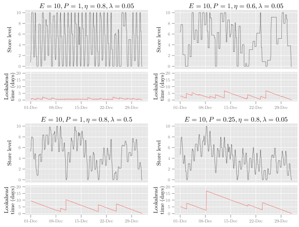
Figure 2: Examples in which the parameters associated with the store are varied. In each case, the upper plot shows the optimal level of storage and the lower plot shows the look-ahead time required at each stage of the optimisation.

The optimal strategy associated with the cost function (26) is shown in Figure 2 (the upper plot in each quadrant) for various choices of parameters. The optimisation takes place over the whole year and we present here the behaviour of the store over a single month (December). The plot in the top-left quadrant corresponds to a “base” case, with the parameter choices $E=10$, $P=1$, $\eta=0.8$ and $\lambda=0.05$. The time $E/P=10$ half-hours units for the store to completely fill or empty and the round-trip efficiency of $0.8$ correspond approximately to the Dinorwig pumped storage facility in Snowdonia in North Wales; since, in the units of this example, the maximum volume which can be bought or sold in a single period is $1$, the choice $\lambda=0.05$ indicates only modest market impact. The upper portion of the plot shows the variation of the store level with time $t$, while the lower portion shows, for each time $t$, the time horizon $\overline{T}_{k}-t$, where $k$ is such that $T_{k-1}+1\leq t\leq T_{k}$, defined in Section 4; the latter is the length of time into the future over which it is necessary to examine the cost functions in order to make the optimal decision at time $t$. It is seen that, under the optimal strategy, the store usually completely empties and fills on a daily cycle, with some lull in activity over the Christmas period. As might be expected the time horizon necessary for an optimal decision is of the order of a day or so.

The plots in the remaining three quadrants of Figure 2 are each formed by varying one of the parameters of the base case example, in each case in such a way that the store is less active. The plot in the top-right quadrant corresponds to a reduction in the round-trip efficiency of the store from $\eta=0.8$ to $\eta=0.6$. Here it is seen that the store level cycles less frequently and tends to remain at the same value for longer periods of time than in the base case—as might be expected; the time horizons necessary for optimal decision making are significantly longer than in the base case. The plot in the lower-left quadrant corresponds to an increase in the “market impact” factor from $\lambda=0.05$ to $\lambda=0.5$, while that in the lower-right quadrant corresponds to a tightening of the rate constraint from $P=1$ to $P=0.25$. In both cases the store is almost continuously active but trades at lower volumes than in the base case; consequently time horizons for optimal decision making are very much longer than in the base case. The broad similarity of the behaviour in these two examples may be explained by noting that an increased market impact factor acts to slow down the activity rate of the store in much the same way as a tightening of the rate constraint. This is because buying prices increase in proportion to the market impact factor with each additional unit of energy bought at that time, whilst selling prices similarly decrease with energy sold. The store therefore needs to balance the benefit of operating at high powers with the impact this has on prices.

For some further numerical results in the context of this particular example, see [12].

7 Stochastic models

In practice there is uncertainty as to future energy prices, and hence there is a need to consider models in which the cost functions $C_{t}$ evolve randomly in time. However, the temporal behaviour of such prices may be very heterogeneous and unlikely to evolve in any stochastically regular manner; thus any comprehensive stochastic modelling of possible future behaviour, together with its optimisation (which under such general circumstances would typically and necessarily involve some form of stochastic dynamic programming) is likely in practice to prove at least computationally infeasible. Thus we should wish to make some form of approximation, sufficiently good as to work well at any time in determining the decision over the next time step; after each such step the future could then be reassessed and the control re-optimised.

There is substantial evidence in the literature that this approach, sometimes referred to as the “rolling intrinsic policy”, often works very well in practice, providing near-optimal strategies at a much lower computational cost than dynamic programming and other competing methods (see, for example, [22] for a comparison of different approximate optimisation methods, both in terms of computational efficiency and accuracy). Examples of cost distributions which have been handled using this approach in the literature, and shown to produce near-optimal results, include (gas) prices whose logarithms evolve as a single-factor, mean-reverting stochastic process [24], and prices which are characterised by multivariate driftless Brownian motions [22, 31]. In [25], a back-casting approach is employed, which can be considered as a special case of the rolling intrinsic policy, in which at each stage of re-optimisation, past prices (from the previous two weeks) are used as future prices. Even under this relatively simple regime, it is illustrated that a store could gain between 80 and 90$\%$ of the profit available in a deterministic setting.

In the present section we propose a stochastic model, in which future uncertainty has a martingale structure (which seems a plausible first approximation to a stochastic structure for price uncertainty). We show that for this model the exact optimal policy is simply that for the deterministic model in which future cost functions are replaced by their expected values, and may thus be determined as in Section 4. In a more general stochastic setting, we propose the following relatively simple strategy: successively at each time step, future cost functions are replaced by their expected values and the present algorithm then used to work out how much to buy or sell in the next time step; future expected cost functions are then re-evaluated prior to the next step. We expect this method to work well, provided that the future expected cost functions, as seen at each re-optimization time $t$, are sufficiently close to the actual costs up until the first time horizon $\overline{T}_{k}$ which follows $t$ (where $\overline{T}_{k}$ is as defined previously). In particular, our analysis in Section 4 shows that, if expected costs exactly match actual costs between times $t$ and $\overline{T}_{k}$, then any uncertainty in costs after $\overline{T}_{k}$ are irrelevant to the decision of the store at time $t$—thus, any inaccuracies arising from this approach are due only to forecasting inaccuracies between times $t$ and $\overline{T}_{k}.$. Given also the relative computational efficiency of the current algorithm, in particular its identification of the shortest time horizon required for the determination of the optimal decision at each time step, we believe that this method should provide a near-optimal procedure for the efficient real-time management of storage over extended periods of time.

Thus we consider a model in which uncertainties in future costs evolve multiplicatively as we proceed backwards in time. (This seems a possible first approximation to market uncertainty.) More precisely we assume that the cost functions $C_{t}$ are given by

$$C_{t}=\xi_{t}\bar{C}_{t},\qquad 1\leq t\leq T,$$

where $(\bar{C}_{1},\dots,\bar{C}_{T})$ is a sequence of deterministic cost functions and where $(\xi_{1},\dots,\xi_{T})$ is a sequence of strictly positive real-valued random variables forming a martingale, i.e. such that

$$\mathbf{E}(\xi_{t}\,|\,\mathcal{F}_{t-1})=\xi_{t-1},\qquad 1\leq t\leq T;$$ (27)

here $\mathbf{E}$ denotes expectation and each $\mathcal{F}_{t}$ is the $\sigma$-algebra generated by $\xi_{1},\dots,\xi_{t}$ (with $\mathcal{F}_{0}$ the trivial $\sigma$-algebra). Note that, since the functions $\bar{C}_{t}$ may if necessary be rescaled, there is no loss of generality in omitting a multiplicative constant from (27). The deterministic functions $\bar{C}_{t}$ are assumed to satisfy the same conditions as the cost functions $C_{t}$ of the deterministic problem given in Section 2, and hence the random cost functions $C_{t}$ also satisfy these conditions.

The optimization problem $\mathbf{P}$ of Section 2 now becomes

• choose the random vector $S=(S_{1},\dots,S_{T})$, with $S_{t}\in\mathcal{F}_{t}$ for each $t$, so as to minimise

  $$G(S):=\mathbf{E}\left[\sum_{t=1}^{T}C_{t}(x_{t}(S))\right]$$ (28)

  with $S_{0}=S^{*}_{0}$ and $S_{T}=S^{*}_{T}$ (where $S^{*}_{0}$ and $S^{*}_{T}$ are fixed constants as previously), and again subject to the capacity constraints

  $$0\leq S_{t}\leq E,\qquad 1\leq t\leq T-1.$$

  and the rate constraints

  $$x_{t}(S)\in X,\qquad 1\leq t\leq T.$$

Note in particular that each $S_{t}$ (or, equivalently, each $x_{t}(S)$) may be chosen based on the knowledge of the realised random variables $\xi_{1},\dots,\xi_{t}$ up to time $t$. We now have the following result (which we reiterate one would expect to use in practice by coupling it with re-optimisation at each time step).

Theorem 6.

The solution to the above problem remains deterministic, with the optimal sequence of store levels as given in the case where stochastic cost functions $C_{t}$ are replaced by their deterministic counterparts $\bar{C}_{t}$. Further the optimized value of the objective function (28) is the same as that for the deterministic variant of the problem.

Remark 3.

This result is intuitively clear, since the stochastic aspect of the problem can be characterised as consisting of, at each successive time, a random but uniform scaling of all future costs, and any such scaling cannot change the optimal strategy. However, a formal proof is required.

Proof of Theorem 6.

Consider first the case in which the stochastic cost functions $C_{t}$ are replaced by their deterministic counterparts $\bar{C}_{t}$. For each $0\leq t\leq T-1$, and each fixed $S_{t}$ such that $0\leq S_{t}\leq E$, with $S_{0}=S^{*}_{0}$, define

$$\bar{V}_{t}(S_{t})=\min_{S_{t+1},\dots,S_{T-1}}\sum_{u=t+1}^{T}\bar{C}_{u}(x_{u}(S)),$$

where $S=(S_{t},\dots,S_{T})$ and, for each $u>t$, we have $0\leq S_{u}\leq E$ with $S_{T}=S^{*}_{T}$ and where $x_{u}(S)=S_{u}-\rho S_{u-1}$ satisfies the rate constraint $x_{u}(S)\in X$. Define also $\bar{V}_{T}(S^{*}_{T})=0$. Thus $\bar{V}_{t}(S_{t})$ represents optimised future costs at time $t$ given that the level of the store is then $S_{t}$. Then, by the usual dynamic programming recursion, we have

$$\bar{V}_{t}(S_{t})=\min_{x_{t+1}\in X}\left[\bar{C}_{t+1}(x_{t+1})+\bar{V}_{t+1}(\rho S_{t}+x_{t+1})\right],\qquad 0\leq t\leq T-1,$$ (29)

where the above minimisation is taken over $x_{t+1}\in X$ such that $0\leq\rho S_{t}+x_{t+1}\leq E$ for $0\leq t\leq T-2$ and $\rho S_{T-1}+x_{T}=E$.

In the general stochastic case define similarly, for $0\leq t\leq T-1$, and each fixed $S_{t}$ such that $0\leq S_{t}\leq E$, again with $S_{0}=S^{*}_{0}$,

$$V_{t}(S_{t})=\mathbf{E}\left[\min_{S_{t+1},\dots,S_{T-1}}\sum_{u=t+1}^{T}C_{u}(x_{u}(S))\,\Bigg{\lvert}\,\mathcal{F}_{t}\right],$$ (30)

where the random vector $S=(S_{t},\dots,S_{T})$ and, for each $u>t$, we have $S_{u}\in\mathcal{F}_{u}$ and $0\leq S_{u}\leq E$ with $S_{T}=S^{*}_{T}$ and where $x_{u}(S)=S_{u}-\rho S_{u-1}\in X$. Define also $V_{T}(S^{*}_{T})=0$. Thus again $V_{t}(S_{t})$ represents optimised future costs at time $t$ given that the level of the store is then $S_{t}$.

We now assert that, for each $t$ and $S_{t}$ as above,

$$V_{t}(S_{t})=\xi_{t}\bar{V}_{t}(S_{t}).$$ (31)

The proof of this assertion is by backwards induction in time $t$. The result is trivially true for $t=T$. Assume now that it is true for $t=u+1$, where $0\leq u\leq T-1$. Then, analogously to (29),

$$V_{u}(S_{u}) =\mathbf{E}\left[\min_{x_{u+1}\in\mathcal{F}_{u+1}}[C_{u+1}(x_{u+1})+V_{u+1}(\rho S_{u}+x_{u+1})]\,\bigg{\lvert}\,\mathcal{F}_{u}\right]$$

$$=\mathbf{E}\left[\min_{x_{u+1}\in\mathcal{F}_{u+1}}\xi_{u+1}[\bar{C}_{u+1}(x_{u+1})+\bar{V}_{u+1}(\rho S_{u}+x_{u+1})]\,\bigg{\lvert}\,\mathcal{F}_{u}\right]$$

$$=\mathbf{E}\left[\xi_{u+1}\bar{V}_{u}(S_{u})\,\bigg{\lvert}\,\mathcal{F}_{u}\right]$$ (32)

$$=\xi_{u}\bar{V}_{u}(S_{u}),$$ (33)

where the above minimisation is taken over $x_{u+1}\in\mathcal{F}_{u+1}$, $x_{u+1}\in X$, and such that $0\leq\rho S_{u}+x_{u+1}\leq E$ with $\rho S_{T-1}+x_{T}=E$ in the case $u=T-1$, and where (32) and (33) follow from (27) and (31) respectively. Hence the assertion (31) holds for all $t$ and for all $S_{t}$.

Note also that, from iteration of the argument leading to (33), for each $t$ and $S_{t}$, the optimising values of $S_{t+1},\dots,S_{T-1}$ are as in the deterministic case. The theorem now follows from this observation and from (31) in the case $t=0$. ∎

8 Commentary and conclusions

In the preceding sections we have developed the optimization theory associated with the use of storage for arbitrage, in particular the strong Lagrangian theory which may be used to form the basis of optimal control and which is necessary for the correct dimensioning of storage facilities. We have also given an algorithm for the determination of the optimal control policy and of the associated Lagrange multipliers. In particular the algorithm captures the fact that the control policy is essentially local in time, in that, for a given system subject to given capacity and rate constraints, at each time optimal decisions are dependent only on future cost functions within an identifiable and typically short time horizon.

Our framework accounts for nonlinear cost functions, rate constraints, storage inefficiencies, and the effect of externalities caused by the activities of the store impacting the market. It further accounts for leakage over time from the store—something which may be expected to substantially further localise over time the character of optimal control policies. While the model of the earlier sections of the paper is deterministic in that it assumes that all the prices determining the cost functions are known in advance, we have also considered what we hope to be a realistic approach to near-optimal control in a stochastic cost environment: the formulation of a reasonably realistic approximate model for which the optimal control may be precisely and efficiently evaluated via the earlier deterministic algorithm, combined with the ability to re-optimise at each time step by reformulating the approximation. This general approach has been shown to work well elsewhere.

What we have not done in the present paper is to consider the use of storage for providing a reserve in case of unexpected system shocks, such as sudden surges in demand or shortfalls in supply. This problem is considered by other authors (see, for example, [5, 15, 16]) in the case where the probabilities of storage underflows or overflows are controlled to fixed levels. However, we believe that a further approach here would be to attach economic values to such underflows or overflows, translating to attaching an economic worth to the absolute level the store (as opposed to attaching a worth to a change in the level of the store as in the present paper). Since in practice storage is used both for arbitrage and for buffering or control as described above, this would provide a more integrated approach to the full economic valuation of such storage.

References

- [1] K. Ahlert and C. Van Dinther. Sensitivity analysis of the economic benefits from electricity storage at the end consumer level. Proc. IEEE Bucharest Power Tech Conf. (2009).
- [2] R.K. Ahuja, T.L. Magnanti and J.B. Orlin. Network Flows: Theory, Algorithms and Applications. Prentice Hall (1993).
- [3] J.P. Barton and D.G. Infield. Energy storage and its use with intermittent renewable energy. IEEE Transactions on Energy Conversion, 19 (2), 441–448 (2004).
- [4] J.P. Barton and D.G. Infield. A probabilistic method for calculating the usefulness of a store with finite energy capacity for smoothing electricity generation from wind and solar power. Journal of Power Sources, 162, 943–948 (2006).
- [5] A.Iu Bejan, R.J. Gibbens and F.P.Kelly. Statistical aspects of storage systems modelling in energy networks. 46th Annual Conference on Information Sciences and Systems (invited session on Optimization of Communication Networks), Princeton University, USA (2012).
- [6] R. Bellman. On the theory of dynamic programming—a warehousing problem. Management Science. 2 (3), 272–275 (1956).
- [7] D. Bertsekas. Dynamic Programming and Stochastic Control. Academic Press (1976).
- [8] D. Bertsekas. Stochastic Optimal Control: the Discrete Time Case. Academic Press (1979).
- [9] S. Boyd and L. Vandenberghe. Convex Optimization. Cambridge University Press (2004).
- [10] A.S. Cahn. The warehouse problem. Bulletin of the American Mathematical Society. 54 (11) 1073-1073 (1948).
- [11] J.R. Cruise, L.C. Flatley and S. Zachary. Impact of storage on energy markets. In preparation (2015).
- [12] J.R. Cruise, R.J. Gibbens and S. Zachary. Optimal control of storage for arbitrage, with applications to energy systems. 48th Annual Conference on Information Sciences and Systems (CISS), 1–6 (2014).
- [13] S.E. Dreyfus. An analytic solution of the warehouse problem. Management Science. 4 (1), 99–104 (1957).
- [14] L. Flatley, R.S. MacKay and M. Waterson. Optimal strategies for operating energy storage in an arbitrage market. http://arxiv.org/abs/1412.0829 (2014)
- [15] N.G. Gast, D.C. Tomozei and J-Y. Le Boudec. Optimal storage policies with wind forecast uncertainties. Greenmetrics 2012, Imperial College, London, UK (2012).
- [16] N.G. Gast, J-Y. Le Boudec, A. Proutiere, and D.C. Tomozei. Impact of storage on the efficiency and prices in real-time electricity markets. Proceedings of the fourth international conference on Future energy systems (2013).
- [17] F. Graves, T. Jenkin and D. Murphy. Opportunities for electricity storage in deregulating markets. The Electricity Journal, 12 (8), 46–56 (1999).
- [18] S.D. Howell, H. Pinto, G. Strbac, N. Proudlove and M. Black. A partial differential equation system for modelling stochastic storage in physical systems with applications to wind power generation. IMA Journal of Management Mathematics, 22, 231–252 (2011).
- [19] W. Hu, Z. Chen and B. Bak-Jensen. Optimal operation strategy of battery energy storage system to real-time electricity price in Denmark. Proc. IEEE Power Energy Soc. Gen. Meet. (2010).
- [20] Y. Huang and S. Mao and R.M. Nelms. Adaptive electricity scheduling in microgrids. Proc. IEEE INFOCOM, Turin, Italy (2013).
- [21] I. Koutsopoulos , V. Hatzi and L. Tassiulas. Optimal energy storage control policies for the smart power grid, Proc. IEEE SmartGridComm, 475–480 (2011).
- [22] G. Lai, F. Margot and N. Secomandi. An approximate dynamic programming approach to benchmark practice-based heuristics for natural gas storage valuation. Operations Research. 58 (3), 564–582 (2010).
- [23] D. Pudjianto, M. Aunedi, P. Djapic and G. Strbac. Whole-systems assessment of the value of energy storage in low-carbon electricity systems. IEEE Transactions on Smart Grid, 5, 1098–1109 (2014).
- [24] N. Secomandi. Optimal commodity trading with a capacitated storage asset. Management Science. 56 (3), 449–467 (2010).
- [25] R. Sioshansi, P. Denholm, T. Jenkin and J. Weiss. Estimating the value of electricity storage in PJM: Arbitrage and some welfare effects. Energy Economics. 31 (2), 269–277 (2009).
- [26] C. Thrampoulidis, S. Bose and B. Hassibi. Optimal large-scale storage placement in single generator single load networks. Power and Energy Society General Meeting (PES), IEEE, 1–5 (2013).
- [27] C. Thrampoulidis, S. Bose and B. Hassibi. Optimal placement of distributed energy storage in power networks. http://arxiv.org/abs/1303.5805 (2013)
- [28] P.M. van de Ven, N. Hegde, L. Massoulié and T. Salonidis. Optimal control of end-user energy storage. IEEE Transactions on Smart Grid, 4, 789–797 (2013).
- [29] P. Whittle. Optimization Under Constraints: Theory and Applications of Nonlinear Programming. Wiley (1971).
- [30] J.C. Williams and B.D. Wright. Storage and Commodity Markets. Cambridge University Press (2005).
- [31] O.Q. Wu, D.D. Wang and Z. Qin. Seasonal energy storage operations with limited flexibility: the price-adjusted rolling intrinsic policy. Manufacturing & Service Operations Management. 14 (3), 455–471 (2012).
-
[32]
https://en.wikipedia.org/wiki/Dinorwig_Power_Station.