Impact of Residual Transmit RF Impairments on Training-Based MIMO Systems

Abstract

Radio-frequency (RF) impairments, that exist intimately in wireless communications systems, can severely degrade the performance of traditional multiple-input multiple-output (MIMO) systems. Although compensation schemes can cancel out part of these RF impairments, there still remains a certain amount of impairments. These residual impairments have fundamental impact on the MIMO system performance. However, most of the previous works have neglected this factor. In this paper, a training-based MIMO system with residual transmit RF impairments (RTRI) is considered. In particular, we derive a new channel estimator for the proposed model, and find that RTRI can create an irreducible estimation error floor. Moreover, we show that, in the presence of RTRI, the optimal training sequence length can be larger than the number of transmit antennas, especially in the low and high signal-to-noise ratio (SNR) regimes. An increase in the proposed approximated achievable rate is also observed by adopting the optimal training sequence length. When the training and data symbol powers are required to be equal, we demonstrate that, at high SNRs, systems with RTRI demand more training, whereas at low SNRs, such demands are nearly the same for all practical levels of RTRI.

I Introduction

MIMO point-to-point systems offer wireless communication with high data rates, without requiring additional bandwidth or transmit power. The pioneering works of [1] and [2] illustrated a linear growth in capacity in rich scattering environments by deploying more antennas at both the transmitter and receiver sides. However, to fully reap the advantages that MIMO systems can offer, instantaneous channel state information (CSI) is essential, especially at the receiver.

In practical systems, a training-based (or pilot-based) transmission scheme is usually utilized to estimate the channel and thereafter to transmit/receive data. This area is well covered in the literature (e.g., [3, 4, 5, 6, 7, 8]); however, most of these works assume ideal RF hardware, which is quite unrealistic in practice. RF impairments, such as in-phase/quadrature-phase (I/Q) imbalance, high power amplifier non-linearities, and oscillator phase noise, are known to have a detrimental impact on practical MIMO systems [9, 10]. Even though one can resort to calibration schemes to mitigate part of these impairments [9], there still remains a certain amount of residual distortions unaccounted for. These residual impairments stem from, for example, inaccurate models which are used to characterize the impairments, as well as, errors in the estimation of impairments’ parameters. To the best of our knowledge, the only paper that considers training-based MIMO systems with residual impairments is [11]. The authors therein analyzed the impact of impairments on the uplink channel estimation in a massive MIMO configuration. They reported an estimation error floor, and observed that by increasing the number of pilot symbols, one can average out the impact of impairments. However, they did not provide detailed power allocation and training sequence schemes, which are of pivotal importance in training-based point-to-point communication systems.

Motivated by the above discussion, we hereafter assess the impact of RTRI on training-based MIMO systems. More specifically, we first evaluate how RTRI affect channel estimation in the estimation phase, and observe an estimation error floor in the high SNR regime, which is analytically deduced. After that, we analyze an approximation for the achievable rate, using the classical technique of [3], in the presence of channel estimation errors, as well as, residual distortions in the data transmission phase. Through optimizing power allocation and training sequence length, we find that, the optimal training duration can be larger than the number of transmit antennas, especially for low and high SNR values. Moreover, for more practical systems, which have the same transmit power per channel use during the estimation and data transmission phases, our results indicate that systems with higher RTRI require more training at high SNRs, whilst at low SNRs, the training demands almost the same for all practical levels of RTRI.

Notation: Upper and lower case boldface letters denote matrices and vectors, respectively. The trace of a matrix is expressed by $\mathrm{tr}\left\{\cdot\right\}$. The $n\times n$ identity matrix is represented by $\mathbf{I}_{n}$. The expectation operation is $\mathbb{E}[\cdot]$, while the matrix determinant is denoted by det$(\cdot)$. The superscripts $(\cdot)^{H}$ and $(\cdot)^{-1}$ stand for Hermitian transposition and matrix inverse, respectively. The Frobenius norm is denoted by $\left\|\cdot\right\|_{F}^{2}$. The symbol $\mathcal{CN}\left(\mathbf{m},\boldsymbol{\Sigma}\right)$ denotes a circularly-symmetric complex multi-variate Gaussian distribution with mean $\mathbf{m}$ and covariance $\boldsymbol{\Sigma}$, while $\triangleq$ refers to “is defined as”.

II Signal and system models

In this paper, we consider a block fading channel with a coherence time of ${T}$ channel uses. During each block, the channel is constant, and is a realization of the uncorrelated Rayleigh fading model. Channel realizations between different blocks are assumed to be independent.

II-A System Model With Residual Transmit RF Impairments

RF impairments exist widely in practical wireless communication systems. Due to these impairments, the transmitted signal is distorted during the transmission processing, hence cause a mismatch between the intended signal and what is actually transmitted. Even though compensation schemes are usually adopted to mitigate the effects of these impairments, there is always some amount of residual impairments. In [9, 10], the authors have shown that these residual impairments on the transmit side act as additive noise. Furthermore, experimental results in [10] revealed that such RTRI behave like zero-mean complex Gaussian noise, but with the important property that their average power is proportional to the average signal power. For sufficient decoupling between different RF chains, such impairments are statistically independent across the antennas. Moreover, impairments during different channel uses are also assumed to be independent. We now denote the RTRI noise as $\boldsymbol{\Delta}$. Then, the input-output relationship of a training-based MIMO system with $N_{t}$ transmit antennas and $N_{r}$ receive antennas within a block of $T$ symbols, can be expressed as

$$\mathbf{Y}=\sqrt{\frac{\rho}{N_{t}}}\mathbf{H}(\mathbf{S}+\boldsymbol{\Delta})+\mathbf{V},$$ (1)

where ${\mathbf{S}}\in\mathbb{C}^{N_{t}\times T}$ is the transmitted signal, $\rho$ is the average SNR at each receive antenna, and $\mathbf{H}\in\mathbb{C}^{N_{r}\times N_{t}}$ is the channel matrix. The receiver noise and the received signal are denoted as $\mathbf{V}\in\mathbb{C}^{N_{r}\times T}$ and $\mathbf{Y}\in\mathbb{C}^{N_{r}\times T}$, respectively. Each element of $\mathbf{H}$ and $\mathbf{V}$ follows an independent $\mathcal{CN}(0,1)$ distribution. We also assume that the entries of $\mathbf{S}$ have unit variance, so that $\rho$ is the average received SNR at each receive antenna. At last, according to the above discussion, we can characterize the RTRI noise $\boldsymbol{\Delta}\in\mathbb{C}^{N_{t}\times T}$ as

$$\boldsymbol{\Delta}_{(i)}\sim\mathcal{CN}\left(\mathbf{0},\delta^{2}\mathbf{I}_{N_{t}}\right),\mathbb{E}\left[\boldsymbol{\Delta}_{(i)}\boldsymbol{\Delta}_{(j)}^{H}\right]=\mathbf{0}$$

$$i,j=1,2,\dots,T,i\neq j,$$ (2)

where $\boldsymbol{\Delta}_{(i)}$ denotes the $i$-th column of $\boldsymbol{\Delta}$. The proportionality parameter $\delta$ characterizes the level of residual impairments in the transmitter. Note that $\delta$ appears in practical applications as the error vector magnitude (EVM) [12], which is commonly used to measure the quality of RF transceivers. For instance, 3GPP LTE has EVM requirements in the range $\left[0.08,0.175\right]$ [12]. The relationship between $\delta$ and EVM is defined as

$$\mathrm{EVM}\triangleq\sqrt{\frac{\mathbb{E}_{\boldsymbol{\Delta}}\left[\left\|\boldsymbol{\Delta}\right\|_{F}^{2}\right]}{\mathbb{E}_{\mathbf{S}}\left[\left\|\mathbf{S}\right\|_{F}^{2}\right]}}=\delta.$$ (3)

When $\delta=0$, it indicates ideal hardware implementation.

We can now decompose the system model in (1) into training phase and data transmission phase as follows:

II-A1 Training Phase

$$\mathbf{Y}_{p}=\sqrt{\frac{\rho_{p}}{N_{t}}}\mathbf{H}\left(\mathbf{S}_{p}+\boldsymbol{\Delta}_{p}\right)+\mathbf{V}_{p},\mathrm{tr}\{\mathbf{S}_{p}^{H}\mathbf{S}_{p}\}=N_{t}T_{p},$$ (4)

where $\mathbf{S}_{p}\in\mathbb{C}^{N_{t}\times T_{p}}$ is the deterministic matrix of training sequences and is known by the receiver, $\rho_{p}$ is the average SNR during the training phase, and $\mathbf{Y}_{d}$ is the $N_{r}\times T_{p}$ received matrix. The distortion noise caused by the RTRI is characterized as

$${\boldsymbol{\Delta}_{p}}_{(i)}\sim\mathcal{CN}\left(\mathbf{0},\delta^{2}\mathbf{I}_{N_{t}}\right),\mathbb{E}\left[{\boldsymbol{\Delta}_{p}}_{(i)}{\boldsymbol{\Delta}_{p}}_{(j)}^{H}\right]=\mathbf{0},$$

$$i,j=1,2,\dots,T_{p},i\neq j.$$ (5)

Note that this model is mathematically similar to the systems which use a superimposed pilot scheme [6], where part of the data symbol is conveyed during the training phase, and acts like noise.

II-A2 Data Transmission Phase

$$\mathbf{Y}_{d}=\sqrt{\frac{\rho_{d}}{N_{t}}}\mathbf{H}\left(\mathbf{S}_{d}\!+\!\boldsymbol{\Delta}_{d}\right)\!+\!\mathbf{V}_{d},\mathbb{E}\Big{[}\mathrm{tr}\{\mathbf{S}_{d}^{H}\mathbf{S}_{d}\}\Big{]}=N_{t}T_{d},$$ (6)

where $\mathbf{S}_{d}\in\mathbb{C}^{N_{t}\times T_{d}}$ is the matrix of data symbols with $\mathcal{CN}(0,1)$ entries, $\rho_{d}$ is the average SNR during the data transmission phase, and $\mathbf{Y}_{d}$ is the $N_{r}\times T_{d}$ received signal matrix. The distortion noise caused by the RTRI during this phase is characterized as

$${\boldsymbol{\Delta}_{d}}_{(i)}\sim\mathcal{CN}\left(\mathbf{0},\delta^{2}\mathbf{I}_{N_{t}}\right),\mathbb{E}\left[{\boldsymbol{\Delta}_{d}}_{(i)}{\boldsymbol{\Delta}_{d}}_{(j)}^{H}\right]=\mathbf{0},$$

$$i,j=1,2,\dots,T_{d},i\neq j.$$ (7)

Recall that conservation of time and energy yields

$$T=T_{p}+T_{d},~{}~{}\rho T=\rho_{p}T_{p}+\rho_{d}T_{d}.$$ (8)

The models in (1), (4), and (6) include the characteristics of RTRI, and enable us to identify some fundamental differences in the training-based MIMO systems as compared to the ideal hardware case of [3].

III LMMSE Channel Estimation

In this section, we analyze the impact of RTRI on the channel estimation phase. Channel estimation is carried out during the first $T_{p}$ channel uses. Within each block, the estimator compares the received signal $\mathbf{Y}_{p}$ with the predefined training sequence matrix $\mathbf{S}_{p}$. The classical results on training-based channel estimation consider Rayleigh fading channels, which have independent complex Gaussian noise with known statistics [3, 7]. However this is not the case herein since the distortion noise $\boldsymbol{\Delta}_{p}$ depends on the unknown random channel $\mathbf{H}$ through the multiplication $\mathbf{H}\boldsymbol{\Delta}_{p}$. Although the distortion noise is Gaussian when conditioned on a channel realization, the effective distortion is the product of Gaussian variables. Thus, it has a complex double Gaussian distribution [13], which does not admit tractable manipulations.

We now derive the LMMSE estimator of $\mathbf{H}$ under the model in (4), which is given by the following lemma.

Lemma 1

Given the received signal $\mathbf{Y}_{p}$ and the RTRI level $\delta$, the LMMSE estimator of $\mathbf{H}$ is

$$\hat{\mathbf{H}}=\mathbf{Y}_{p}\bigg{(}\mathbf{S}_{p}^{H}{\mathbf{S}_{p}}+\left(\delta^{2}\rho_{p}+1\right)\mathbf{I}_{T_{p}}\bigg{)}^{-1}\mathbf{S}_{p}^{H}.$$ (9)

Proof:

Since the rows of $\mathbf{Y}_{p}$ are independent and identically distributed (i.i.d.), we can write the LMMSE estimator in the general form $\hat{\mathbf{H}}=\mathbf{Y}_{p}\mathbf{A}$, where $\mathbf{A}$ should minimize the mean square error (MSE), which is defined as $\mathrm{MSE}\triangleq\mathrm{tr}\left(\mathbf{C}_{e}\right)$. Herein, $\mathbf{C}_{e}\!\triangleq\!\mathbb{E}\left[\mathbf{H}_{e}^{H}\mathbf{H}_{e}\right]$ is defined as the estimation error covariance matrix, where $\mathbf{H}_{e}\triangleq\mathbf{H}-\hat{\mathbf{H}}$ is the estimation error matrix. The estimator in (9) is found by taking the first derivative of the MSE with respect to $\mathbf{A}$, and equating the result to zero. ∎

Corollary 1

The training sequence matrix $\mathbf{S}_{p}$ that minimizes the MSE should satisfy

$$\mathbf{S}_{p}\mathbf{S}_{p}^{H}=T_{p}\mathbf{I}_{N_{t}}$$ (10)

and the corresponding MSE is given by

$$\mathrm{MSE}=\frac{N_{r}N_{t}}{1+g}~{}\mathrm{with}~{}g\triangleq\frac{\rho_{p}T_{p}}{N_{t}(\rho_{p}\delta^{2}+1)}.$$ (11)

Proof:

This corollary can be proved by applying the Lagrange multiplier method [14] on the MSE, subject to the power constraint $\mathrm{tr}\{\mathbf{S}_{p}^{H}\mathbf{S}_{p}\}=N_{t}T_{p}$. The resulting estimation error covariance matrix becomes

$$\mathbf{C}_{e}=\frac{N_{r}}{1+g}\mathbf{I}_{N_{t}}.$$ (12)

Since $\mathbf{H}_{e}$ has zero mean, the variance of its entries can be expressed as $\sigma_{\mathbf{H}_{e}}^{2}=\frac{1}{N_{r}N_{t}}\mathrm{tr}\{\mathbf{C}_{e}\}=\frac{1}{1+g}$, which is also defined as the normalized MSE. By the orthogonality principle of LMMSE estimators [15], each element in $\hat{\mathbf{H}}$ has a variance of $\sigma_{\hat{\mathbf{H}}}^{2}=1-\sigma_{\mathbf{H}_{e}}^{2}=\frac{g}{1+g}$. ∎

Figure 1 shows the normalized MSE, $\sigma_{\mathbf{H}_{e}}^{2}$, of a $4\times 4$ MIMO system for different levels of impairments. In this case, we use $T_{p}\!=\!4$ channel uses to transmit pilot symbols, which is the minimum length required to estimate all channel dimensions. Without the existence of RTRI, increasing the transmit power decreases the MSE monotonically towards zero. However, in the presence of RTRI, we observe a fundamentally different behavior. Specifically, when the transmit power becomes high, impairments will generate an irreducible error floor, which is explicitly provided in the following corollary.

Corollary 2

Asymptotically as $\rho_{p}\!\rightarrow\!\infty$, the normalized MSE approaches the limit

$$\mathrm{MSE}_{\mathrm{normalized}}^{\rho_{p}\!\rightarrow\!\infty}=\frac{1}{1+\frac{T_{p}}{N_{t}\delta^{2}}}.$$ (13)

Proof:

This corollary is simply achieved by making $\rho_{p}$ in (11) large and normalize the MSE with respect to the number of transmit and receive antennas. ∎

Obviously, the value of this floor depends on the level of impairments; in general, large RTRI will cause severe degradation of the channel estimates. We can also see from (13) that, for a fixed level of RTRI, an increase in the training sequence length $T_{p}$ decreases the MSE monotonically. As expected, for low SNR values, impairments have only limited impact, which is in line with the results of [11].

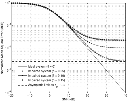
Figure 1: Normalized mean square error (MSE) for different levels of impairments ($N_{t}=N_{r}=4,T=100,T_{p}=4$).

IV Data Transmission

This section analyzes the achievable rate of the non-ideal training-based MIMO system. The results in [3], under the assumption of ideal hardware, are frequently used as reference.

During the data transmission phase, the estimated channel $\hat{\mathbf{H}}$ is available at the receiver. The receiver uses $\hat{\mathbf{H}}$ as if it were the true channel realization to recover the intended signal $\mathbf{S}_{d}$. Recalling that $\mathbf{H}\!=\!\hat{\mathbf{H}}\!+\!\mathbf{H}_{e}$, we may rewrite the received signal as

$$\mathbf{Y}_{d} =\sqrt{\frac{\rho_{d}}{N_{t}}}\hat{\mathbf{H}}\left(\mathbf{S}_{d}+\boldsymbol{\Delta}_{d}\right)+\sqrt{\frac{\rho_{d}}{N_{t}}}\mathbf{H}_{e}\left(\mathbf{S}_{d}+\boldsymbol{\Delta}_{d}\right)+\mathbf{V}_{d}$$

$$=\sqrt{\frac{\rho_{d}}{N_{t}}}\hat{\mathbf{H}}\mathbf{S}_{d}\!+\!\underbrace{\sqrt{\frac{\rho_{d}}{N_{t}}}\left(\hat{\mathbf{H}}\boldsymbol{\Delta}_{d}\!+\!\mathbf{H}_{e}\mathbf{S}_{d}\!+\!\mathbf{H}_{e}\boldsymbol{\Delta}_{d}\right)\!+\!\mathbf{V}_{d}}_{\tilde{\mathbf{V}}},$$ (14)

where $\tilde{\mathbf{V}}$ is the “effective noise” matrix. Note that each entry of $\tilde{\mathbf{V}}$ has zero-mean and the variance

$$\sigma_{\tilde{\mathbf{V}}}^{2}=\frac{1}{N_{r}T_{d}}\mathbb{E}\left[\mathrm{tr}\left\{{\tilde{\mathbf{V}}^{H}}\tilde{\mathbf{V}}\right\}\right]=\left(\frac{1}{1+g}+\delta^{2}\right)\rho_{d}+1.$$ (15)

On a similar note, we can define $\bar{\mathbf{H}}\!\!\triangleq\!\!\tiny{\frac{1}{\sigma_{\hat{\mathbf{H}}}^{2}}}\!\hat{\mathbf{H}}$, which has uncorrelated and approximately $\mathcal{CN}(0,1)$ entries.

Given that $\hat{\mathbf{H}}$ is known to the receiver, it is straightforward to prove that $\mathbf{S}_{d}$ and $\tilde{\mathbf{V}}$ are uncorrelated. From [3], we know that the worst-case effective noise is circularly-symmetric complex Gaussian distributed, with the same covariance as $\tilde{\mathbf{V}}$, Then, we can straightforwardly obtain a capacity lower bound as in [3, Theorem 1].

In the considered case though, where the channel estimate (9) contains the multiplicative term $\mathbf{H}\boldsymbol{\Delta}_{p}$, $\hat{\mathbf{H}}$ is only approximately Gaussian. Then, we can work out the approximated achievable rate according to

$$\tilde{R}=\frac{T_{d}}{T}\mathbb{E}\left[\mathrm{log_{2}}\ \mathrm{det}\!\left(\mathbf{I}_{N_{r}}+\rho_{\mathrm{eff}}\frac{\bar{\mathbf{H}}\bar{\mathbf{H}}^{H}}{N_{t}}\right)\right],$$ (16)

where $\rho_{\mathrm{eff}}$ denotes the effective SNR,

$$\rho_{\mathrm{eff}} \triangleq\frac{\rho_{d}\sigma_{\hat{\mathbf{H}}}^{2}}{\sigma_{\tilde{\mathbf{V}}}^{2}}$$ (17)

$$=\frac{\rho_{d}\rho_{p}T_{p}}{N_{t}(1+\rho_{p}\delta^{2})(1+\rho_{d}+\rho_{d}\delta^{2})+\rho_{p}T_{p}+\rho_{d}\rho_{p}T_{p}\delta^{2}}.$$ (18)

IV-A Optimizing over Power Allocation

First, we optimize the power allocation to maximize the effective SNR $\rho_{\mathrm{eff}}$.

Let $\alpha$ denote the fraction of the total transmit power that is assigned to the data transmission phase. Then, we have

$$\rho_{d}T_{d}=\alpha\rho T,~{}\rho_{p}T_{p}=(1-\alpha)\rho T,~{}0<\alpha<1.$$ (19)

Proposition 1

The optimal power allocation $\alpha\!\triangleq\!\frac{\rho_{d}T_{d}}{\rho T}$ in a training-based MIMO system with RTRI is given by

$$\alpha^{\mathrm{opt}}=\begin{cases}\frac{r-\sqrt{r^{2}-rs}}{s},&\textrm{for $s\neq 0$}\\ \frac{1}{2},&\textrm{for $s=0$}\end{cases}$$ (20)

where for concision, we have defined

$$r \triangleq\rho T+\frac{N_{t}\rho T\delta^{2}}{T_{p}}+N_{t},$$

$$s \triangleq\rho T+\frac{N_{t}\rho T\delta^{2}}{T_{p}}-\frac{N_{t}\rho T(1+\delta^{2})}{T_{d}}.$$

Proof:

Substituting $\rho_{p}\!=\!\frac{(1-\alpha)\rho T}{T_{p}}$ and $\rho_{d}\!=\!\frac{\alpha\rho T}{T_{d}}$ into (18), then taking the first and second derivatives of $\rho_{\mathrm{eff}}$ with respect to $\alpha$ and equating the result to be zero, the proof follows immediately. ∎

Specifically, for high and low SNRs, we have

Corollary 3

At high and low SNRs, the optimal power allocation $\alpha$ reduces to

• At high SNRs, as $\rho\rightarrow\infty$

  $$\alpha^{\mathrm{opt}}=\frac{\left(1+\frac{N_{t}\delta^{2}}{T_{p}}\right)\left(1+\sqrt{\frac{N_{t}(1+\delta^{2})}{T_{d}}}\right)}{1+\frac{N_{t}\delta^{2}}{T_{p}}-\frac{N_{t}(1+\delta^{2})}{T_{d}}},$$ (21)

• At low SNRs, as $\rho\rightarrow 0$

  $$\alpha^{\mathrm{opt}}=\frac{1}{2}.$$ (22)

Clearly, at low SNR, half of the transmit power should be assigned to the training phase, which is consistent with the results of [3]. With the help of (20), we can further optimize the training length to maximize the approximated achievable rate.

IV-B Optimizing over $T_{p}$

In this part, we seek to determine the optimal training length $T_{p}$. Recall from [3] that, for ideal hardware systems over i.i.d. Rayleigh fading channels, it is always optimal to use as few channel uses as possible (i.e., $N_{t}$) for pilot symbols, regardless of the values of $\rho$ and $T$. However, for non-ideal hardware systems, we will show that this is no longer the case, since the optimal training length could be larger than $N_{t}$.

The standard way of finding the optimal training sequence length $T_{p}$ requires to substitute the optimal power allocation scheme $\alpha^{\mathrm{opt}}$ back to the approximated achievable rate in (16), and then take the derivative of $\tilde{R}$ with respect to $T_{p}$. Unfortunately, this is not analytically tractable. To overcome this problem, we first derive the approximated achievable rate in (16) in closed-form, which only depends on the values of SNR and $T_{p}$ for a given system setup ($N_{t}$, $N_{r}$, and $T$). Then, for each value of SNR, we can perform an exhaustive search over the integer $T_{p}$ to find the global optimum.

To facilitate our analysis, we herein present the following proposition.

Proposition 2

The approximated achievable rate in (16), is analytically given by

$$\begin{split}\tilde{R}&=\frac{qKT_{d}}{{\ln(2)T}}\sum\limits_{n=1}^{q}{\sum\limits_{m=1}^{q}{{{\left({-1}\right)}^{n+m}}\det\left(\boldsymbol{\Omega}\right)}}\Gamma\left(t\right)e^{\frac{N_{t}}{\rho_{\mathrm{eff}}}}\\ &\times\sum\limits_{k=1}^{t}{\frac{\Gamma\left(-t+k,\frac{N_{t}}{\rho_{\mathrm{eff}}}\right)}{{\left(\frac{\rho_{\mathrm{eff}}}{N_{t}}\right)}^{t-k}}}\end{split}$$ (23)

where $q\triangleq\min(N_{r},N_{t})$, $p\triangleq\max(N_{r},N_{t})$ and $t\triangleq n+m+p-q-1$. Also, ${K}=\left[\prod_{i=1}^{q}(p-i)!\prod_{j=1}^{q}(q-j)!\right]^{-1}$ is a normalization constant. Moreover, $\Gamma(x)$ and $\Gamma(y,z)$ denote the Gamma function [16, Eq. (8.310.1)] and the upper incomplete Gamma function [16, Eq. (8.350.2)], respectively. Finally, $\boldsymbol{\Omega}$ is a $(q-1)\times(q-1)$ matrix whose $(i,j)$-th element is given by

$$\boldsymbol{\Omega}_{i,j}=\left(\gamma_{i,j}^{(n)(m)}+p-q\right)!\,q^{-\frac{1}{q-1}}$$

where

$$\gamma_{i,j}^{(n)(m)}\triangleq\begin{cases}i+j-2,&\textrm{if $i<n$ and $j<m$}\\ i+j,&\textrm{if $i\geq n$ and $j\geq m$}\\ i+j-1,&\textrm{otherwise.}\end{cases}$$ (24)

Proof:

We can rewrite (16) as

$$\tilde{R}=\frac{T_{d}}{T}\mathbb{E}\left[\mathrm{log_{2}det}\left(\mathbf{I}_{q}+\frac{\rho_{\mathrm{eff}}}{N_{t}}\mathbf{W}\right)\right],$$ (25)

where $\mathbf{W}$ is defined as

$$\mathbf{W}\triangleq\begin{cases}\bar{\mathbf{H}}\bar{\mathbf{H}}^{H},&\textrm{if $N_{r}\leq N_{t}$},\\ \bar{\mathbf{H}}^{H}\bar{\mathbf{H}},&\textrm{if $N_{r}>N_{t}$}.\end{cases}$$ (26)

Note that $\mathbf{W}$ is a $q\times q$ random, non-negative definite matrix following the complex Wishart distribution. Thus, it has real non-negative eigenvalues and the probability density function (PDF) of its unordered eigenvalue, $\lambda$, is found in [17, Eq. (38)] to be

$$p_{\lambda}(\lambda)=K\sum\limits_{n=1}^{q}\sum\limits_{m=1}^{q}\frac{(-1)^{m+n}\lambda^{n+m+p-q-2}}{e^{\lambda}}\det\left({\boldsymbol{\Omega}}\right).$$ (27)

By exploiting the eigenvalue properties, we can now alternatively express the approximated achievable rate in (25) as

$$\tilde{R}=\frac{qT_{d}}{T}\int\limits_{0}^{\infty}\log_{2}\left(1+\frac{\rho_{\mathrm{eff}}}{N_{t}}\lambda\right)p_{\lambda}(\lambda)d\lambda.$$ (28)

This integral can be evaluated using the integral identity in [18, Eq. (40)]. The expression in (23) then follows after some simple algebraic manipulations. ∎

Based on (23), we perform an exhaustive search over the integer $T_{p}$ for different SNR values. Figure 2 compares the optimal training sequence length, $T_{p}^{\mathrm{opt}}$, for the ideal and impaired systems. For the ideal hardware system, the optimal training length is always equal to the number of transmit antennas, which has already been proved in [3]. For the non-ideal hardware systems with RTRI, however, the optimal training sequence length may become larger than $N_{t}$. Generally speaking, higher impairment levels impose longer training sequences. At high SNRs, the effective SNR saturates, thus the overall performance cannot be improved by increasing the power; however, we can benefit by extending the training period. This is because the total pilot power is spread over $T_{p}$ channel uses, hence the impact of the temporally uncorrelated RTRI will be averaged over $T_{p}$ as well. It is also worth mentioning that in the low SNR regime, where thermal noise dominates the system performance, there is still an increase in achievable rate by improving the channel estimation with longer training sequences. The above results are valid for different number of antennas, and can be extended to massive MIMO systems with large receive antenna arrays.

In Fig. 3, we have plotted the approximated achievable rate with the optimal power allocation scheme. For each SNR value, we choose the best training sequence length $T_{p}^{\mathrm{opt}}$. It is noteworthy that, for the hardware impaired systems, the achievable rate saturates when SNR becomes high, even though we have used the optimized scheme. This behavior remains even if we have perfect CSI as in [19], thus it is a fundamental effect of hardware impairments. In Fig. 4, we plot the relative rate gain by adopting the optimal training sequence length $T_{p}^{\mathrm{opt}}$. The relative rate gain is defined as

$$\textrm{relative~{}rate~{}gain}\triangleq\frac{R_{T_{p}^{\mathrm{opt}}}-R_{T_{p}=N_{t}}}{R_{T_{p}=N_{t}}}\times 100\%,$$ (29)

where $R_{T_{p}^{\mathrm{opt}}}$ and $R_{T_{p}=N_{t}}$ refer to the approximated achievable rate (23) when $T_{p}$ obtains its optimal value and $T_{p}\!=\!N_{t}$, respectively. We can conclude from this figure that, the relative rate gain provided by utilizing the optimal training sequence length, varies according to the level of RTRI. Systems with higher level of impairments benefit far more from the optimization over $T_{p}$.

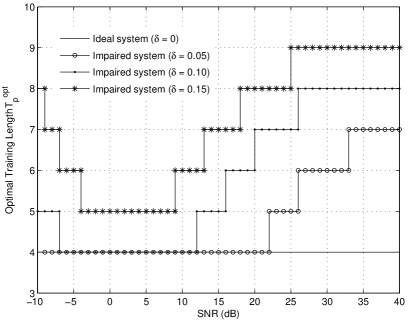
Figure 2: Optimal training sequence length for different levels of impairments when both power allocation and training sequence length are optimized ($N_{t}=N_{r}=4,T=100$).

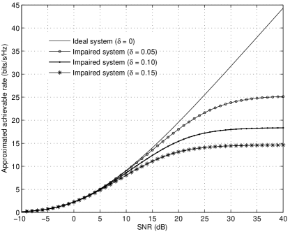
Figure 3: The approximated achievable rate when both power allocation and training sequence length are optimized ($N_{t}=N_{r}=4,T=100$).

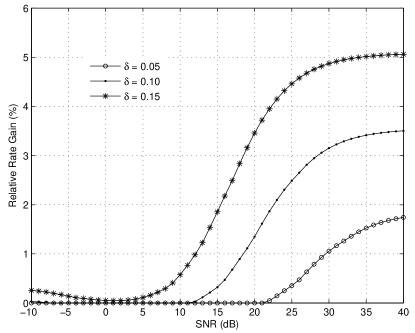
Figure 4: The relative rate gain by adopting the optimal training sequence length, compared to the case of using training sequence of length $N_{t}$ ($N_{t}=N_{r}=4,T=100$).

IV-C Equal Training and Data Power

In practice, communication systems do not often have the freedom of varying the transmit powers during the training phase and data transmission phase. As such, the transmit power for pilot and data symbols is always the same, i.e., $\rho_{p}=\rho_{d}=\rho$. In this case, the effective SNR in (18) becomes

$$\rho_{\mathrm{eff}}=\frac{\rho^{2}T_{p}}{N_{t}(1+\rho\delta^{2})(1+\rho+\rho\delta^{2})+(\rho^{2}\delta^{2}+\rho)T_{p}}.$$ (30)

The corresponding analytical approximated achievable rate follows straightforward by inserting (30) into (23). Using the obtained analytical rate expression, we can, once more, resort to exhaustive search to find the optimal training sequence length.

Figure 5 depicts the optimal $T_{p}$ for a $4\times 4$ MIMO system with coherence time $T=100$. As we can see, for all cases, the demand for training is especially high at low SNRs, whilst this demand decreases as the SNR scales up. Generally speaking, higher level of RTRI require longer training length in the high SNR regime, whereas such demands are nearly the same for all practical levels of impairments at low SNRs.

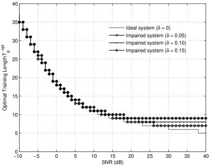
Figure 5: Optimal training sequence length for different levels of impairments when only the training sequence length is optimized ($N_{t}=N_{r}=4,T=100,\rho_{p}=\rho_{d}=\rho$).

V Conclusions

In this paper, we analyzed the impact of residual transmit RF impairments on training-based MIMO systems. We derived a new LMMSE channel estimator for systems with RTRI, and then found that such residual impairments create an irreducible estimation error floor. Moreover, the optimal power allocation scheme and optimal training sequence length were thereafter investigated. We showed that the optimal training sequence length may be larger than the number of transmit antennas, and increases with the level of impairments. An increase in the relative rate is observed by adopting the optimal training sequence length. We also investigated the optimal training sequence length when there is no freedom of varying the transmit power during the estimation and data transmission phases, and concluded that the demand for training is the same at low SNRs, while more training was needed at high SNRs when the system experiences RTRI.

References

- [1] E. Telatar, “Capacity of multi-antenna Gaussian channels,” Europ. Trans. Telecom., vol. 10, no. 6, pp. 585–595, Nov.-Dec. 1999.
- [2] G. J. Foschini and M. J. Gans, “On limits of wireless communications in a fading environment when using multiple antennas,” Wireless Pers. Commun., vol. 6, no. 3, pp. 311–335, Mar. 1998.
- [3] B. Hassibi and B. M. Hochwald, “How much training is needed in multiple-antenna wireless links?” IEEE Trans. Inf. Theory, vol. 49, no. 4, pp. 951–963, Apr. 2003.
- [4] L. Tong, B. M. Sadler, and M. Dong, “Pilot-assisted wireless transmissions: General model, design criteria, and signal processing,” IEEE Signal Process. Mag., vol. 21, no. 6, pp. 12–25, Nov. 2004.
- [5] M. Biguesh and A. B. Gershman, “Training-based MIMO channel estimation: A study of estimator tradeoffs and optimal training signals,” IEEE Trans. Signal Process., vol. 54, no. 3, pp. 884–893, Mar. 2006.
- [6] M. Coldrey and P. Bohlin, “Training-based MIMO systems–Part I: Performance comparison,” IEEE Trans. Signal Process., vol. 55, no. 11, pp. 5464–5476, Nov. 2007.
- [7] E. Björnson and B. Ottersten, “A framework for training-based estimation in arbitrarily correlated Rician MIMO channels with Rician disturbance,” IEEE Trans. Signal Process., vol. 58, no. 3, pp. 1807–1820, Nov. 2010.
- [8] M. Agarwal, M. L. Honig, and B. Ata, “Adaptive training for correlated fading channels with feedback,” IEEE Trans. Inf. Theory, vol. 58, no. 8, pp. 5398–5417, Aug. 2012.
- [9] T. Schenk, RF Imperfections in High-Rate Wireless Systems: Impact and Digital Compensation. Springer, 2008.
- [10] C. Studer, M. Wenk, and A. Burg, “MIMO transmission with residual transmit-RF impairments,” in Proc. ITG/IEEE Work. Smart Ant. (WSA), Feb. 2010, pp. 189–196.
- [11] E. Björnson, J. Hoydis, M. Kountouris, and M. Debbah, “Massive MIMO systems with non-ideal hardware: Energy efficiency, estimation, and capacity limits,” IEEE Trans. Inf. Theory, 2013, submitted, arXiv:1307.2584.
- [12] H. Holma and A. Toskala, LTE for UMTS: Evolution to LTE-Advanced. Wiley, 2011.
- [13] N. O’Donoughue and J. Moura, “On the product of independent complex Gaussians,” IEEE Trans. Signal Process., vol. 60, no. 3, pp. 1050–1063, Mar. 2012.
- [14] D. P. Bertsekas, Nonlinear programming. Athena Scientific, 1999.
- [15] S. M. Kay, Fundamentals of Statistical Signal Processing, Volume 1: Estimation theory. Prentice Hall PTR, 1993.
- [16] I. S. Gradshteyn and I. M. Ryzhik, Table of Integrals, Series, and Products, 7th ed. Academic Press, 2007.
- [17] A. Zanella, M. Chiani, and M. Z. Win, “On the marginal distribution of the eigenvalues of Wishart matrices,” IEEE Trans. Commun., vol. 57, no. 4, pp. 1050–1060, Apr. 2009.
- [18] M. Kang and M.-S. Alouini, “Capacity of MIMO Rician channels,” IEEE Trans. Wireless Commun., vol. 5, no. 1, pp. 112–122, Jan. 2006.
- [19] E. Björnson, P. Zetterberg, M. Bengtsson, and B. Ottersten, “Capacity limits and multiplexing gains of MIMO channels with transceiver impairments,” IEEE Commun. Lett., vol. 17, no. 1, pp. 91–94, Jan. 2013.