Constraining parameters of white-dwarf binaries using gravitational-wave and electromagnetic observations
Abstract
The space-based gravitational wave (GW) detector, evolved Laser Interferometer Space Antenna (eLISA) is expected to observe millions of compact Galactic binaries that populate our Milky Way. GW measurements obtained from the eLISA detector are in many cases complimentary to possible electro-magnetic (EM) data. In our previous papers, we have shown that the EM data can significantly enhance our knowledge of the astrophysically relevant GW parameters of the Galactic binaries, such as the amplitude and inclination. This is possible due to the presence of some strong correlations between GW parameters that are measurable by both EM and GW observations, for example the inclination and sky position. In this paper, we quantify the constraints in the physical parameters of the white-dwarf binaries, i.e. the individual masses, chirp mass and the distance to the source that can be obtained by combining the full set of EM measurements such as the inclination, radial velocities, distances and/or individual masses with the GW measurements. We find the following fractional uncertainties in the parameters of interest. The EM observations of distance constrains the the chirp mass to , whereas EM data of a single-lined spectroscopic binary constrains the secondary mass and the distance with factors of 2 to . The single-line spectroscopic data complemented with distance constrains the secondary mass to . Finally EM data on double-lined spectroscopic binary constrains the distance to . All of these constraints depend on the inclination and the signal strength of the binary systems. We also find that the EM information on distance and/or the radial velocity are the most useful in improving the estimate of the secondary mass, inclination and/or distance.
Subject headings:
stars: binaries - gravitational waves, Galactic binaries - GW parameters, GW detectors - LISA1. Introduction
Gravitational wave (GW) observations and electro-magnetic (EM) observations can be used to study compact Galactic binaries independently and often these two ways provide different measurements of the same system. There are about 50 of these binaries that have been studied in the optical, UV, and X-ray wavelengths (e.g. Roelofs et al., 2010). This number is expected to grow by a factor of 100 (Nissanke et al., 2012) when a space-based gravitational wave (GW) observatory like the recently eLISA111In preparation by ESA, expected launch in 2034 will be in operation. This detector is expected to observe millions of compact Galactic binaries with periods shorter than about a few hours (Nelemans, 2009; Amaro-Seoane et al., 2013), amongst other astrophysical sources. Of those millions of binaries we will be able to resolve several thousands. It has been shown (Shah et al., 2012, Paper I, hereafter) that for a non-eclipsing binary system (for example AM CVn), its EM measurement of the inclination, can improve the error on the GW amplitude () significantly depending on the strength of the GW signal and the magnitude of the EM uncertainty in the inclination. is a GW parameter which is given by a combination of the masses, orbital period and distance to the source:
| (1) |
where, is the distance to the source, is the source’s GW frequency (), and is the chirp mass defined as:
| (2) |
From the GW observations alone, one typically cannot measure the individual masses or the distance since they are degenerate via Eqs. 1, 2. In the rare cases that a precise orbital decay (), can be measured from GW data then the distance can be estimated (with the assumption that the frequency evolution is dictated by GW radiation only) by determining from the measured and via the equation (Peters & Mathews, 1963):
| (3) |
For the compact binaries that have been observed with the optical telescopes, a subset of which will also be detected by eLISA, their EM data often provide measurements of the orbital period , the primary mass (), sometimes the secondary mass (), the distance () and the radial velocity amplitude (). We use these measurements for a few binaries to show the quantitative improvements in their GW and other physical parameters. Many of these binaries can/could still be found electromagnetically before or after eLISA discoveries.
We have previously shown that knowing sky positions from EM data can improve the GW uncertainties on and depending on the particular geometry and orientation of the binary systems (Shah et al., 2013). Thus, so far we have quantitatively studied the improvement factors in the uncertainties of the parameters that can be gained from prior knowledge of parameters which are common to both GW and EM observations, for example inclination, and sky position.
In this paper we go beyond constraining only those GW parameters which are also measured independently from the EM data. We explore various combinations of any possible EM observations and the GW measurements in constraining the useful parameters of the binaries that are astro-physically interesting, for example the individual masses. Because their GW signal is significantly affected we consider high-inclination (sometimes eclipsing) and (low inclination) binary systems. We review the GW data analysis methods in Sect. 2. In Sect. 3, we explore the information gained by combining EM measurements in different ways where the EM data can be the radial velocity of one of the binary components, , , , and . Specifically, we classify various combinations into a number of scenarios in discussing the parameter constraints.
| [rad] | [Hz] | [rad] | [rad] | ||||||
|---|---|---|---|---|---|---|---|---|---|
| J0651 | a, b | a, b | a, b |
-
a
for , kpc
-
b
for , kpc
2. Parameter uncertainties from GW observations
For our analyses below, we consider one of the eLISA verification binaries J065133.33+284423.3 (J0651, hereafter; Brown et al. (2011)). We also consider a second (hypothetical) system with higher masses which we will refer to as “the high mass binary”. Their GW parameter values are listed in Table 1. Before looking at the EM data we briefly recap out GW data analysis method. We have used Fisher matrix studies (e.g Cutler, 1998) to extract the GW parameter uncertainties and correlations in the GW parameters that describe the compact binary sources. Our method and application of Fisher information matrix (FIM) for eLISA binaries together with their signal modeling and the noise from the detector and the Galactic foreground have been described in detail in Paper I. Most of the binaries will be monochromatic sources and such sources are completely characterized by a set of seven parameters, dimensionless amplitude (), frequency (), polarization angle (), initial GW phase (), inclination (), ecliptic latitude (), and ecliptic longitude (). From the GW signal of a binary and a Gaussian noise we can use FIM to estimate the parameter uncertainties. The inverse of the FIM is the variance-covariance matrix whose diagonal elements are the GW uncertainties and the off-diagonal elements are the correlations between the two parameters. We do the GW analyses of the above mentioned binaries for eLISA observations of two years. We note that Fisher-based method is a quick way of computing parameter uncertainties and their correlations in which these uncertainties are estimated locally at the true parameter values and therefore by definition the method cannot be used to sample the entire posterior distribution of the parameters. Additionally Fisher-based results hold in the limit of strong signals with a Gaussian noise (e.g. Vallisneri, 2008, see also Appendix).
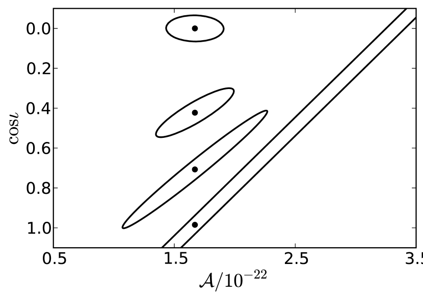
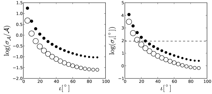
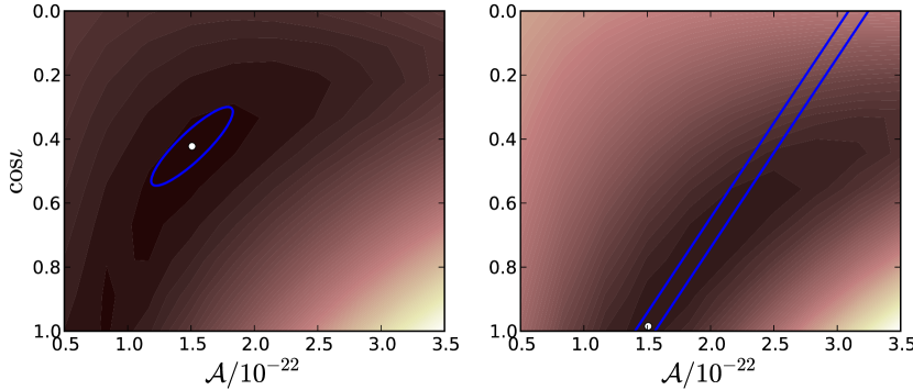
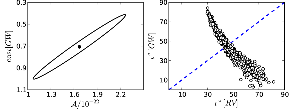
The two-dimensional GW distribution in amplitude and inclination given by the variance-covariance matrix for J0651 parameters are shown in Figure 1 for a number of inclinations. The largest and most highly correlated distribution is that with and the weakest correlation is that with . The behavior of these distributions reflect the strength of the correlation between amplitude and inclination. As discussed in Paper I, the low inclination systems have very similar signal shapes, whereas systems with high inclinations are distinguishable by both the shape and structure for small differences in inclinations. Thus, for low-inclination binaries a small change in is indistinguishable from a small change in its . On the other hand for high-inclination binaries a small change in inclination produces a noticeably different signal explaining the uncertainties in and becoming large to small with increasing inclination. The GW uncertainties for the amplitude and inclination as a function of inclination are shown in Figure 2 for J0651 (in filled circles) and the high mass binary (in open circles). The strong increase in uncertainty trends for low inclination systems is due to the correlation between amplitude and inclination (Shah et al., 2012). Clearly the high mass binary has larger S/N which gives smaller uncertainties in both of its parameters shown in open circles in the figure compared to that of J0651. Observe that inclination is a cyclic parameter and is bounded between and yet we get very large uncertainties from Fisher matrix for lower inclinations systems shown in the right panel of in Figure 1. This is due to the fact that Fisher matrix methods are based on the linearised signal approximation as a result of which it is not sensitive to the bounded parameters that describe the signal model (Vallisneri, 2008). In other words in FIM one computes the uncertainties in parameters based on variation of the signal with respect to the parameters at the true parameter values and the fact that far away from the true value the parameter has a bound is not taken into account by the FIM. When the uncertainty in a bounded parameter exceeds its physically allowed range, it means the quantity cannot be determined from GW data analysis. The dashed line in in Figure 2 indicates the value (at ) beyond which the uncertainties in imply unphysical values for the inclination. Since the low inclination systems on the left-side of the plot are affected by this, corrections have to be applied to the corresponding (over-estimated) uncertainties in amplitude in the left panel by discarding the unphysical range in the inclination (Shah et al., 2013). One way to correct these unphysical values is by taking a rectangular prior on the inclination. This in effect will cut off the posterior distribution in the parameters at the physical bounds described by the prior. Note that cutting off the error ellipses at lower inclinations in Figure 1 is reasonable because taking strict bounds far away form the real value about which Fisher uncertainties are computed will not change the shape and slope significantly. The cut off in the posterior distributions due to rectangular priors will skew the means of the paramter distributions away from the real value (Rodriguez et al., 2013, Eq. C4). Furthermore we stress the fact that the Fisher matrix method is an estimate and cannot, follow the posterior in detail (see Appendix).
The normalized correlations between all the seven parameters for an eclipsing and non-eclipsing orientations of J0651 are listed in the variance-covariance matrices (VCM) in the Appendix. We will make use of these parameter uncertainties and their corresponding correlations when combining with various EM data in Sect. 3.
2.1. GW information only
We start by considering the case where we only have the GW data. From the GW observations, the astrophysical parameters of interest for a monochromatic source are its , and . From the GW data analysis the frequency of the source will be very well determined, Hz (e.g. Paper I) for a Hz source, so we consider that is essentially known with a fixed value. Given that most of the binaries that we will observe with eLISA will be binary white-dwarfs (WD) (Nelemans et al., 2001), we can restrict their masses to . For simplicity we take uniform distributions for both masses in this range. This provides a distribution in the system’s chirp mass, which will provide an upper limit on the distance for the source. In Figure 3 we show these estimates in with their percentile (or uncertainties) as a function of inclination for both J0651 (in black) and for the high mass binary with equal high-mass components (in grey). The dashed line (in black) is the real value of the distance for both systems. The lower medians of distances at the lower inclinations for both systems are explained by the fact that at , the GW distribution of has a long uniform tail. This is shown in Figure 4 where we compare the distributions of for two inclinations: (in black), and (in grey) in the left panel. For a fixed distribution of , the corresponding distributions in are shown in the right panel where the solid vertical lines are the distribution medians and dashed vertical line is the real value. We can see that thus giving
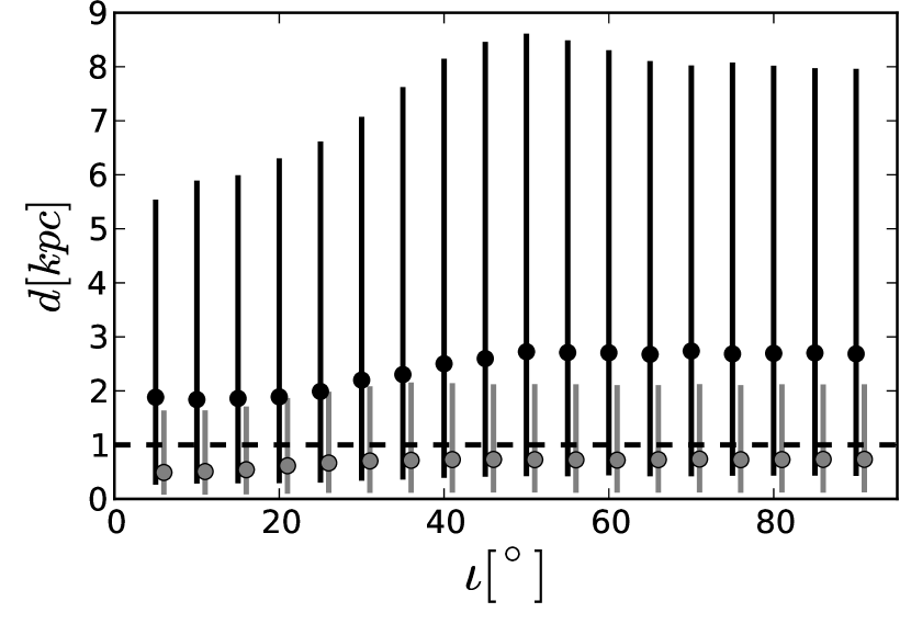
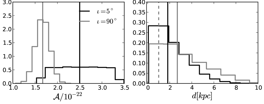
via Eq. 1 for a fixed . Also, observe that the median distances are over-estimated for J0651 for all inclinations and this is because the real value of the median in is much smaller than that computed from uniform distributions in , which is the same for all inclinations. Whereas for the high mass binary the computed median in is close to its real value thus translating into smaller offsets in the median distances in Figure 3. In the figure, the percentiles in the distance slightly increase as a function of inclination even though the uncertainties in has the opposite behavior (see Figure 2). This is because the has a very large fractional uncertainty compared to that of the and thus the relative error uncertainties in the chirp mass dominates those in the distance, which remain roughly constant for all inclinations.
3. Combining EM & GW observations
In all the various scenarios we analyze below, we take the EM parameters with an uncertainty of which is inspired by observational uncertainties of J0651. This binary is a well known EM source and also a guaranteed source for eLISA. J0651 is an eclipsing system and such an orientation of a nearby binary allows accurate EM measurements of it’s orbital parameters, and the masses (accuracies of (primary mass); (secondary mass)) from observing the spectra, radial velocities and eclipses of each star by the other (Brown et al., 2011). Furthermore its rate of change of orbital period has also been measured from follow-up high speed photometry from yr. worth of data to an accuracy of (Hermes et al., 2012), and this will improve in the course of time. In this section we classify specific (possible) scenarios where we could have one or more EM data on the white dwarf binary parameters. We explicitly state how much the knowledge of any of the various parameters that describe the physical properties of a binary system can be further improved if we can fold in various combinations of the existing EM and/or GW observations. We construct three specific scenarios below based on the typical knowledge from the EM observations:
-
•
EM data on distance
-
•
Single-line spectroscopic data (complemented with or without the distance measurement)
-
•
Double-line spectroscopic data
In all the scenarios the GW information on amplitude, inclination and frequency from Sect. 2.1 are used.
3.1. Scenario 1: EM observation of the distance
Measuring distances accurately is made feasible by the Gaia mission (de Bruijne, 2012), a new astrometric satellite. Gaia is expected to measure stellar parallaxes of millions of stars with arcsec accuracy depending on how bright a star is. For example at 1 kpc, J0651 (g = 19.1 mag) would have a arcsec accuracy in the parallax measurement corresponding to a fractional accuracy in distance of (e.g. Bailer-Jones, 2009). There is also some indication of the distance of the binary from its absolute magnitude. The uncertainties in from such measurements are also of the order of several percent or for the case of J0651(Brown et al., 2011).
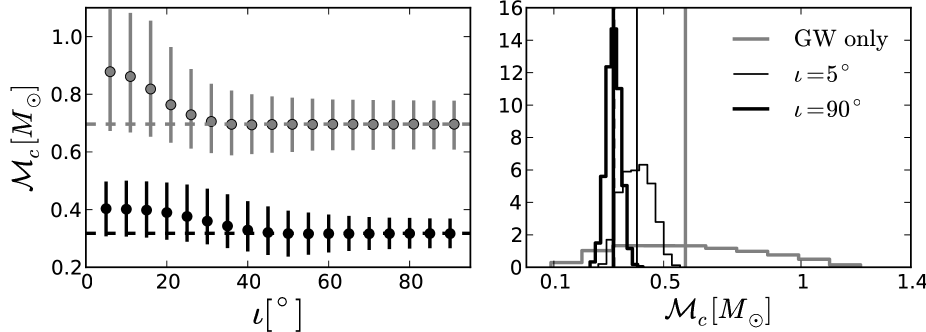
A sole EM measurement of the distance of a WD binary might be possible in cases where the system is identified as a WD binary but it is too faint to measure other parameters. For instance from the wide-field surveys it is often possible to identify WD from their colors (Verbeek et al., 2013). Given the distance and the GW uncertainty in amplitude, we can trivially solve for the chirp mass, using Eq. 1. The resulting probability distribution functions (pdf) are computed by randomly drawing points from the given distributions and computing the parameter of interest for each draw. The percentiles in the are shown in the left panel of Figure 5 for J0651 (in black) and the high mass binary (in grey) as a function of inclination. The dashed lines (in black for J0651 and in grey for the high mass binary) are the real values. The decreasing medians of the chirp mass with inclination follows from the GW distributions in the amplitude that is shown in Figure 4 where the median is overestimated for (in thin black lines) compared to that of (in thick black lines). For a fixed distribution in distance the corresponding distribution of is therefore overestimated for shown in the right panel of Figure 5 compared to that of . The percentiles of the chirp masses for both J0651 and the high mass binary are affected by these overestimated medians of the amplitudes at lower inclinations which cause significant offsets of the from their respective real values as can be seen in the left panel of Figure 5. Thus at lower inclinations where the medians in the amplitude are overestimates, the percentiles in the chirp mass can be interpreted as upper limits of the chirp mass. In order to calculate reliable constraints in at these small inclinations we have to do full (Bayesian) data analyses that takes into account the physical priors and gives us a better estimate of the expected posterior distributions in the desired parameters. The percentile in for both systems decrease as a function of inclination as is expected from the propagation of uncertainty where . Thus, knowing distance from EM observation gives us an estimate of the chirp mass where the constraints are tighter for the higher inclination (eclipsing) systems.
3.2. Scenario 2: EM observations of single-lined spectroscopic binary
Some measurements are unique to EM observations such as the radial velocity , of one of the components () of the binary:
| (4) |
which can be used to measure inclination. We adopt the convention from the optical studies of the binary sources where the primary mass, is the brighter object and the dimmer secondary mass, . Note that the inclination measurement from the GW data analysis, and from the radial velocity equation above i.e. are two independent measurements for the same system. We will show that these two are anti-correlated below in Sect. 3.2.3, yielding radial velocity measurements very useful.
3.2.1 Scenario 2a: EM data on
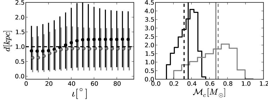
Before looking at a real single-lined spectral binary we first consider the case that only the mass is known from the EM data. This is a viable scenario when determining is impossible and we may get an estimate of the primary mass from the photometry or the spectra. Assuming a double WD system, we take a uniform distribution for , which together with the given constrains the . The estimates of distance with their corresponding percentiles as a function of inclination are shown in Figure 6 for both the J0651 (in black) and the high mass binary (in grey). The real value of distance is shown in the dashed (black) line. The offsets of the medians in the distance at low inclinations for both the binary systems can be explained in a similar way as in the previous sections, which is due to the overestimated medians of at lower inclinations as shown in the left panel of Figure 4. Additionally, the significant discrepancy between the median distance for J0651 vs. the high mass binary (at ) is again due to the over-estimated value of the for J0651 assuming a uniform distribution distribution. This is shown in the right panel of Figure 6 where the vertical dashed lines are their corresponding true values of the and the vertical solid lines are the medians of the corresponding distributions. The simulated distribution of from an EM measurement of with a Gaussian width in its uncertainty together with an assumed uniform distribution in the unknown results in an overestimated median of the for J0651 compared to that of the high mass binary. This propagates in overestimating the median for J0651 at higher inclinations unlike for the high mass binary since its median is slightly underestimated. The flat priors on is affecting this and if we already know the secondary mass is low, we may take a distribution in weighted towards lower masses and that will affect the constraints obtained in the . The constraints in the distance from Figure 6 can be compared with those in Figure 3 where there was no EM information on any of the masses: the upper limits on for both J0651 and the high mass binary are constrained by a up to factor of better when is known for both binaries with accuracy.
3.2.2 Scenario 2b: EM data on &
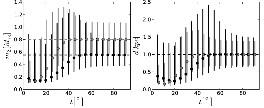
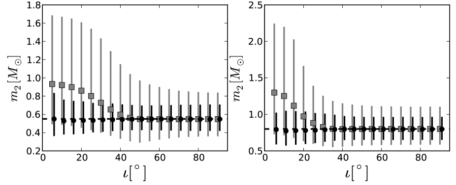
In this case we consider EM measurements of a single-lined spectroscopic binary where resolving one of the masses of the binary spectroscopically typically provides measurements on the primary mass and its radial velocity. We assume an uncertainty in radial velocity amplitude of corresponding to the typical accuracy of km/s found in the EM measurements (for e.g., Roelofs et al., 2006). Given and from the EM data and inclination from GW data , we can numerically solve for via the formulation in Eq. 4. Assuming it is a WD, the is restricted to lie in . Then a fixed pair of [, ] and the masses give us a distance. We calculate the resulting distributions in and the distance from the Gaussian distributions of and about their typical EM uncertainties and GW distributions in the inclination and amplitude. The percentile in the secondary mass and the distance are shown in Figure 7 as a function of inclination for both J0651 (in black) and the high mass binary (in grey). Like in the scenarios discussed above, for the lowest inclinations, the over estimated FIM uncertainties of propagates into erroneous constraints on , and . Thus, at lower inclinations we have to use Bayesian methods to get their accurate GW uncertainties. Observe that the percentile in the and the distance roughly similar and large from . This is again due to the influence of the GW distributions in at the lower inclinations, which have uniform distributions resulting into over-estimated medians (see Figure 1). However, for the uncertainties for both , and decrease with inclination and their medians stabilize at the true values. This is caused by the fact that at higher inclinations, the medians of GW amplitudes are close to the true values of the systems where the constraints on the GW parameters are also tighter with increasing inclination. Thus, the decreasing uncertainties in as a function of (see right panel of Figure 2) should result in the same behavior of via Eq. 4. Since distance is computed using these , the same behavior holds for the distance in the right panel.
3.2.3 Scenario 2c: EM data on , &
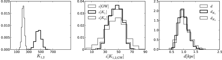
Here the EM measurements of a single-lined spectroscopic binary in the previous subsection is complemented with a distance measurement from Gaia or from an estimate of the absolute magnitude. From the primary mass , distance and the amplitude we immediately get the secondary mass, . We will call this as the preliminary since this can be further improved by folding in the radial velocity measurement. As mentioned before the radial velocity measurement essentially provides an independent measurement of the inclination via Eq. 4. This can be seen in the following way: The GW parameters of the non-eclipsing J0651 are: whose VCM uncertainties are: , and rad respectively. We also take a fixed radial velocity, corresponding to , (listed in Table 1), and . The 2-d Gaussian distribution from GW data with uncertainties for these parameters is shown in the left panel of Figure 8. For each randomly selected pair of and for a fixed , and , we can solve for the from Eq. 1. Using this for that fixed and , we solve for . For many points randomly picked in the space the computed are compared with the corresponding in the right panel. The inclinations measured in two ways roughly anti-correlate. However we know that values of that are different from cannot be true. Thus, constraining the inclination of the system in a small area around along the diagonal line in the right panel also constrains and the amplitude. We make use of this in the case considered in this subsection. The preliminary and their percentiles computed from EM data on , , and the GW data on as a function of inclination is shown in Figure 9 in grey lines in the left panel for J0651. The same for the high mass binary is also shown in the right panel in grey lines. From this , given , and , the radial velocity, is computed which is compared with the from the EM data. Since the EM measured is more precise, we keep the subset of those and the respective weighted with a probability distribution function of the given by:
| (5) |
The final reduced percentiles in are shown in black lines for J0651 in left panel, and the same is shown for the high mass binary in the right panel. Observe that the uncertainties in calculated in this way for lower inclinations is the similar to those at the higher inclinations. Thus, the advantage of folding in measurement is especially useful for lower inclination systems with S/N , where large GW uncertainties influence the constraints of the physical parameters in question. Furthermore, the constraints in can also be compared with the previous case in Figure 7 where we find that for the single-lined spectroscopic binary, knowing its distance to significantly improves knowledge of the secondary mass at lower inclinations.
The key point in Scenarios 2b and 2c is that not all the pairs are consistent with the EM observations. Therefore both constraints on the GW data and other parameters also constrain the GW error ellipses. The uncertainties in the GW amplitude and GW inclination for these scenarios are shown in the Appendix.
3.3. Scenario 3: EM data on , , &
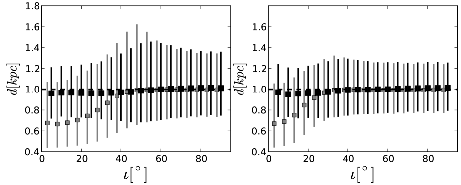
In this section we consider EM observations of a double-lined spectroscopic binary which translates to a set of measurements in the mass and radial velocity for each of the components: , , and , . Given the two masses and GW measurement on the amplitude we can immediately compute a preliminary distance. Additionally, we can also derive two sets of inclinations independently from the individual radial velocities and the masses, from Eq. 4. These inclinations can be compared with the one measured from GW data, . At lower inclinations, large uncertainties in essentially imply that those systems’ inclinations are undetermined and this also affects the amplitude due to the strong correlation between them. Thus, the independent estimates of from the EM data can be useful in constraining the GW amplitude. This reduced amplitude will further constrain the distance which is shown in the third panel in Figure 10. In the figure both the observed are shown in the left panel in thick and thin black lines respectively. The inclination and the distance given the GW amplitude and both the masses are shown in grey line in the middle and right panels respectively. Both the inclination and distance derived from and are plotted in thick and thin black lines respectively. Observe that a fractional error in each and translate into similar uncertainties of the distance and thus in the following figures we show the constraints from using data only. The constrained distances estimated in this way as a function of inclination is shown in Figure 11 for J0651 in left panel (also in black) and for the high mass binary in the right panel (in black). The grey lines in both the panels are the percentiles in using only the masses from the EM data and the GW amplitude. Observe that at lower inclinations knowing masses and a radial velocity can improve the constraint in distances significantly. The uncertainties are smaller for J0651 at lowest inclinations because the relative uncertainties in the have lower absolute uncertainties that propagate into the uncertainties of the distance.
Note that typically in practice EM data provides measurements of both the masses and only one of the radial velocities with precision. From the radial velocity formulation we have the relation: relation which can be used to compute the remaining . This provides a consistency check between EM and GW data. The EM data can be used to derive inclination measured from the radial velocities, which can be verified against the as shown in the middle panel in Figure 10.
4. Conclusions
We have quantified the possible constraints/improvements in the physical parameters of the white-dwarf (WD) binaries that are observable by the eLISA detector in the future when combined with the EM data. We do this for the binary parameters that are astrophysically interesting (masses and distance). For the GW observations from eLISA, we calculate the source’s variance-covariance matrix using the Fisher methods where the Galactic binary source is described by seven parameters (or eight if is measurable). We have taken J0651 and a higher mass binary in our analyses where J0651 is a verification source for eLISA. We consider various possible cases depending on the availability of the EM measurements and combine those with GW uncertainties in the amplitude and inclination in order to solve for the unknown parameters as a function of inclinations for both J0651 and the high mass binary. For clarity we list all the cases below:
-
1.
GW data only: Assuming a double white-dwarf system this scenario somewhat constrains the distance.
-
2.
Scenario 1: GW data + distance : This scenario constrains the chirp mass .
-
3.
Scenario 2a: GW data + primary mass : This scenario constrains the chirp mass and the distance.
-
4.
Scenario 2b: GW data + single-lined spectroscopic binary i.e. , : This scenario constrains the secondary mass and the distance.
-
5.
Scenario 2c: GW data + single-lined spectroscopic binary + : This scenario also constrains the secondary mass .
-
6.
Scenario 3: GW data + double-lined spectroscopic binary i.e. , and , : This scenario constrains the distance.
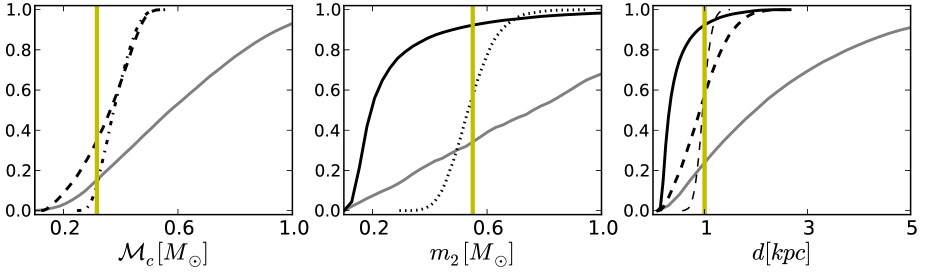
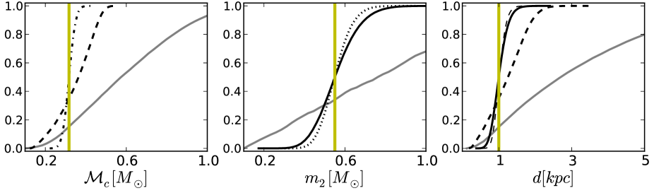
All the EM accuracies are taken to be of the real/measured values which is inspired by several EM observations. We compare below the constraints in the physical parameters of interest: secondary mass , chirp mass and the distance as a function of the scenarios depending on the EM information available. Since the GW parameter uncertainties are significantly different for a low inclination (face-on) orientation than for a high inclination (edge-on) orientation, we do the comparison for a non-eclipsing J0651 with and an almost eclipsing J0651 with in Figures 12 and 13 respectively and conclude the following:
-
1.
Constraints on chirp mass, : In the left panels of Figures 12 and 13, EM data on constrains the 95 percentile of the system’s chirp mass (dash-dotted line) to and for face-on and eclipsing J0651 respectively. EM data on constraints the (in thick-dashed line) to which does not depend on the inclination. The normalized cumulative distributions (CDF) of the constraints on the distance are compared to that from GW data only which is shown in the grey line in both panels.
-
2.
Constraints on secondary mass, : In the middle panels of Figures 12 and 13, EM data on the constrain the 95 percentile of secondary mass, to and for face-on and eclipsing J0651 respectively (shown in solid lines). The same set of data complemented with the distance further constrain the 95 percentile in with and for face-on and eclipsing J0651 respectively (shown in dotted lines). For comparison, the CDF of using only the GW data is shown in grey.
-
3.
Constraints on distance, d: In the right panels, of Figure 12 and 13, EM data on constrains the distance to kpc and kpc for face-on and eclipsing J0651 respectively (in thick-dashed lines). EM data on the constrain the 95 percentile in with kpc and with kpc accuracy for face-on and eclipsing J0651 respectively (in solid lines). EM data on and constrain the 95 percentile in to kpc and kpc for face-on and eclipsing J0651 respectively (in thin-dashed line). For comparison, the CDF of using only the GW data and the assumption that the masses are WDs is shown in grey.
Thus, knowing distance and/or radial velocity of the primary component can significantly improve our knowledge of the binary system. These constraints change as a function of inclination of the binary that is shown in previous sections. In a forthcoming paper we will address the effect on these improvements by including the (possible) EM measurement of rate of change of the orbital period.
References
- Amaro-Seoane et al. (2013) Amaro-Seoane, P., Aoudia, S., Babak, S., et al. 2013, GW Notes, Vol. 6, p. 4-110, 6, 4
- Bailer-Jones (2009) Bailer-Jones, C. A. L. 2009, in IAU Symposium, Vol. 254, IAU Symposium, ed. J. Andersen, Nordströara, B. m, & J. Bland-Hawthorn, 475–482
- Brown et al. (2011) Brown, W. R., Kilic, M., Hermes, J. J., et al. 2011, ApJ, 737, L23
- Cutler (1998) Cutler, C. 1998, Phys. Rev. D, 57, 7089
- de Bruijne (2012) de Bruijne, J. H. J. 2012, Ap&SS, 341, 31
- Hermes et al. (2012) Hermes, J. J., Kilic, M., Brown, W. R., et al. 2012, ApJ, 757, L21
- Nelemans (2009) Nelemans, G. 2009, Classical and Quantum Gravity, 26, 094030
- Nelemans et al. (2001) Nelemans, G., Yungelson, L. R., & Portegies Zwart, S. F. 2001, A&A, 375, 890
- Nissanke et al. (2012) Nissanke, S., Vallisneri, M., Nelemans, G., & Prince, T. A. 2012, ApJ, 758, 131
- Peters & Mathews (1963) Peters, P. C., & Mathews, J. 1963, Physical Review, 131, 435
- Rodriguez et al. (2013) Rodriguez, C. L., Farr, B., Farr, W. M., & Mandel, I. 2013, Phys. Rev. D, 88, 084013
- Roelofs et al. (2006) Roelofs, G. H. A., Groot, P. J., Nelemans, G., Marsh, T. R., & Steeghs, D. 2006, MNRAS, 371, 1231
- Roelofs et al. (2010) Roelofs, G. H. A., Rau, A., Marsh, T. R., et al. 2010, ApJ, 711, L138
- Shah et al. (2013) Shah, S., Nelemans, G., & van der Sluys, M. 2013, A&A, 553, A82
- Shah et al. (2012) Shah, S., van der Sluys, M., & Nelemans, G. 2012, A&A, 544, A153
- Vallisneri (2008) Vallisneri, M. 2008, Phys. Rev. D, 77, 042001
- Verbeek et al. (2013) Verbeek, K., Groot, P. J., Nelemans, G., et al. 2013, MNRAS, 434, 2727
Appendix A Variance-covariance matrixes of J0651
We have listed the VCM matrices for the J0651 system with eclipsing
and non-eclipsing configurations in
our analysis. There are 7 parameters that describe them which are
listen in the first row of the matrices below and for each binary, the
values are listed in the row with . The diagonal elements
are the absolute uncertainties in each the 7 parameters and the
off-diagonal elements are the normalized correlations, i.e.
The strong correlations between parameters (i.e. whose magnitudes are
) are marked in bold in the VCMs below. These correlations
have been explained in Paper I.
VCM 1: Eclipsing J0651 (), S/N .
A ϕ0cosιf ψsinβλθi( 1.67×10⁻²²π0.0072.61×10-3π/2-0.08 2.10) A 0.08×10⁻²³-0.00.00.010.020.03-0.06ϕ00.907-0.01-0.910.010.110.08cosι0.1720.01-0.010.07-0.33f 2.982×10⁻¹⁰-0.01-0.08-0.15ψ0.035-0.020.05sinβ0.0590.08λ0.017
VCM 2: Not-eclipsing J0651 (), S/N .
A ϕ0cosιf ψsinβλθi( 1.67×10⁻²³π0.7072.61×10-3π/2-0.08 2.10) A 3.86×10-230.03-0.98-0.020.03-0.130.35ϕ00.739-0.03-0.190.160.150.10cosι0.190.02-0.010.13-0.36f 1.688×10⁻⁹-0.98-0.06-0.21ψ0.360.130.07sinβ0.031-0.13λ0.009
Appendix B Constraints in and of J0651
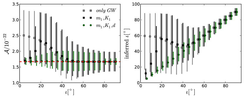
Figure 14 shows how the error ellipses of amplitude and inclination from GW observations reduce using EM observations for the different scenarios that we have described in Sects. 1 and 2. Knowing one of the masses (Scenario 2a) from the EM does not constrain the any more than the GW data alone. In other words the and are free parameters to satisfy the amplitude. The percentiles in the amplitude are shown in grey in the figure which are the same as the case where we have GW data only. In fact these constraints in the amplitude decrease as a function of inclination as expected from the GW measurements (see Figure 2). Adding an EM measurement of the measured mass’s radial velocity (Scenario 2b) can constrain the slightly or significantly depending on inclination of the system which are shown in thick black lines. Finally complementing the mass and radial velocity of the brighter companion with the distance to the binary (Scenario 2c) significantly constraints the which is strongest for the lower inclinations as shown in the figure in thin black lines. Observe that EM information provide strongest improvements for low inclination systems where GW uncertainties in the amplitude and the inclination are very large.
Appendix C The distribution of and at lower inclinations
Here we show that while Fisher method gives an estimate on the parameter uncertainties and correlation between them without following the posterior in detail, it gives a reasonable estimate of the above quantities as long as the priors in the parameters are rectangular (i.e. not Gaussian) and are large enough to preserve the overall orientation of the posterior. We compute an estimate of the likelihood with a simple procedure on a 2D parameter distribution of and , where the , = true signal, = signal at a grid point and is a noise realisation, total time samples. For an evenly placed parameters in a grid, we take the average computed for 10 different noise realisations. Figure 15 shows the colored contours of 2D distribution for the case of (in the left-panel) where the Fisher uncertainties are well within the physically allowed bounds. The over-plotted contour in thick solid line is uncertainty ellipse computed from Fisher matrix about the true values of and labelled with the white circle. This just shows that the distribution follows the shape and the slope of the Fisher distribution roughly, but not exactly as expected. The same is shown for in the right-panel where the uncertainties hit the physical bounds and both the methods show a sharp cut-off at . Here we see that again the Fisher uncertainties and correlation roughly follow that of the , but with truncations at the boundaries. The deviation in the top-right is discussed in Shah et al. (2012). It was argued that although the results of Fisher-based uncertainties imply that the system is very similar to , this is unlikely because of the anti-correlation between and at high inclinations. At correlation between and decreases and the high accuracy in the inclination itself actually suffices to distinguish the higher inclination systems. Thus we expect that that deviates from the Fisher estimate towards the top-right region of the Figure 15 in the right-panel.