Strongly interacting mesoscopic systems of anyons in one dimension

Abstract

Using the fractional statistical properties of so-called anyonic particles, we present solutions of the Schrödinger equation for up to six strongly interacting particles in one-dimensional confinement that interpolate the usual bosonic and fermionic limits. These solutions are exact to linear order in the inverse coupling strength of the zero-range interaction of our model. Specifically, we consider two-component mixtures of anyons and use these to eludicate the mixing-demixing properties of both balanced and imbalanced systems. Importantly, we demonstrate that the degree of demixing depends sensitively on the external trap in which the particles are confined. We also show how one may in principle probe the statistical parameter of an anyonic system by injection a strongly interacting impurity and doing spectral or tunneling measurements.

I Introduction

In the quantum world we classify physically identical particles according to their statistical properties and typically divide them into two distinct sets. The key characteristic is that upon exchange of two such particles the total wave function changes only by a sign which is positive for bosonic and negative for fermionic particles. It came as quite a surprise to many when Leinass and Myrheim lm1977 (see also Refs. wilczek1982, ; goldin1981, ) discovered that in two dimensions (2D) one can accomodate exchange statistics that is neither bosonic nor fermionic but rather interpolates the usual possibilities and gives rise to so-called anyonic particles. Systems that display effective anyonic statistics are a topic of great current interest due to the integral role they enjoy in the field of quantum computation pachos2012 (see Ref. sarma2008, for an overview of recent theoretical and experimental progress).

An early breakthrough in the understanding of anyons was achieved by Haldane who generalized the 2D case and introduced the notion of ’fractional statistics’ in any dimension haldane1991 . Anyons also play a prominent role in exploring the connection between statistical mechanics and random matrix theory alonso1996 ; jain1997 . In one dimension (1D), the famous Calogero-Sutherland (CS) model calogero1969 ; sutherland1971 provides an example of fractional statistics and anyons poly1989 . The CS model can even be extended to exactly solvable many-body models exhibiting long-range order in 1D auberson2000 . Thus, 1D anyonic systems remains a research topic of great interest in several different fields zhu1996 ; kundu1999 ; batchelor2006 ; girar2006 ; averin2007 ; feiguin2007 ; patu2007 ; trebst2008 ; campo2008 ; fidkowski2008 ; greiter2009 ; santa2008 ; bellazzini2009 ; santos2012 . Most recently, realization of anyonic behavior in cold atomic gases have been proposed in both 2D paredes2001 ; aguado2008 ; jiang2008 and 1D keilmann2011 setups. Such proposals typically require manipulation of small atom numbers. It is therefore encouraging that preparation of desired mesoscopic system sizes is becoming increasingly more precise serwane2011 ; wenz2013 ; pellegrino2014 ; nogrette2014 .

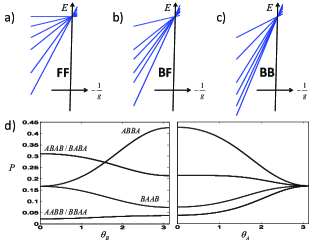
Figure 1: (Color online) Four-body system of two $A$ and two $B$ particles in a hard-wall box with statistical parameters $\theta_{A}$ and $\theta_{B}$ respectively. The exact solution for large short-range interaction strength, $g$, have linear spectral slopes as shown schematically for a) Fermi-Fermi (FF), b) Bose-Fermi (BF), and c) Bose-Bose (BB) mixtures. d) The probabilities of different particle configurations for the ground state is shown as a function of first $\theta_{B}$ (keeping $\theta_{A}=0$) and then $\theta_{A}$ (keeping $\theta_{B}=\pi$). The particle configurations of each line is shown in the left-hand panel. The system is dominantly antiferromagnetic in the FF limit ($\theta_{B}=\theta_{A}=0$), then becomes demixed in the BF case ($\theta_{B}=\pi$ and $\theta_{A}=0$), and finally becomes completely mixed in the BB limit ($\theta_{B}=\theta_{A}=\pi$) where all configurations are equally likely.

In this paper we will utilize the notion of anyons to elucidate the behavior of strongly interacting mesoscopic 1D systems. In particular, we will describe a general framework that can deal with mixtures of several components of anyonic particles with the important limiting cases being Fermi-Fermi, Bose-Fermi, and Bose-Bose systems. Using solutions of the Schrödinger equation for the up to six-body systems in both box and harmonic confinement, we will show how statistics and trapping potentials are important for the tendency of two-component systems to either mix or phase separate when the particles have strong short-range repulsive interactions. This mixing-demixing transition remains a very active research area with several open questions das2003 ; cazalilla2003 ; adilet2006 ; fang2011 ; wang2012 . The results we present quantify exactly what one should understand by demixing at the level of particle ordering in the exact wave functions that take the full trap geometry into account and thus go beyond any local density approximation based on Bethe ansatz, mean-field, or Luttinger liquid theory.

The solutions of the Schrödinger equation are obtained based on a recently developed functional approach to systems with strong zero-range interactions parametrized by a coupling strength $g$. The solutions we present are exact to linear order in $1/g$. It does not rely on Bose-Fermi girardeau1960 ; cheon1999 ; girar2004 ; girar2010 or Anyon-Fermi mappings girar2006 as these techniques are not capable of solving general multi-component systems vol2013 . In contrast, our approach yields energies and wave functions that are adiabatically connected to the eigenstates for large by finite interaction strengths. In Fig. 1 we show an example with four particles in a hard-wall box (open boundary conditions) for different particle statistics (to be defined below). In order to reach the strongly interacting (’hard core’) regime one typically tunes the interaction strength from weak to strong in experimental setups. It is therefore essential to provide theoretical predictions that take the preparation into account. This is not possible if one starts from the strictly impenetrable so-called Tonks-Girardeau tonks1936 ; girardeau1960 regime where all manipulations are done assuming an infinite short-range repulsion. Our framework naturally provides suggestions for probing anyonic statistics in strongly interacting systems through both the energy spectra and the particle ordering contained in the wave functions. As a concrete example we consider using a strongly interacting impurity in a tunneling experiment to infer the statistical properties of the majority particles.

II Model

The model Hamiltonian for our $N$-body system has the form

$$H=\sum_{i}\left[-\frac{\hbar^{2}}{2m}\frac{\partial^{2}}{\partial x_{i}^{2}}+V(x_{i})\right]+g\sum_{i<j}\delta(x_{i}-x_{j}),$$ (1)

where $m$ is the mass, $V(x)$ is the external trap potential, and $g$ is the interaction strength. Here we assume that all particles have the same mass and the same interaction strength which is always parametrized by $g$. The trap potential length scale is $L$ (box size or harmonic trap length) which is our basic unit throughout. From $L$ we obtain $\hbar^{2}/mL^{2}$ as our unit of energy and likewise we will measure $g$ in units of $\hbar^{2}/mL$. The anyonic exchange symmetry implies that girar2006

$$\Psi(x_{k},x_{k+1})=-e^{-i\theta\epsilon(x_{k+1}-x_{k})}\Psi(x_{k+1},x_{k}),$$ (2)

where we suppress the dependence on all $N$ coordinates for simplicity and $x_{k}$ and $x_{k+1}$ are two adjacent identical (anyonic) particles that we exchange and $\epsilon(x)=-\epsilon(-x)=1$ ($\epsilon(0)=0$). For $\theta=0$ they are fermions (F) and for $\theta=\pi$ they are bosons (B). The boundary conditions are dictated by $V(x)$. It is open boundary conditions, i.e. $\Psi$ vanishes at the end of the box for the hard-wall case, while for the harmonic trap one has gaussian decay at large distance. Periodic boundary conditions are not discussed here.

When we discuss two-component mixtures below it is important to note that there are no symmetry requirements between different components, i.e. the wave function may acquire an arbitrary phase under exchange of an $A$ and a $B$ particle. In Ref. santos2012 , solutions with symmetric (bosonic) exchange of $A$ and $B$ particles have been discussed. We obtain the eigenstates of the Hamiltonian without restrictions on the exchange of $A$ and $B$. These eigenfunctions can have different phases under exchange of $A$ and $B$, but they are nevertheless eigenstates and thus the physically relevant states.

A powerful feature of our approach to strongly interacting systems vol2013 , is that we obtain these states without using the representation theory of symmetry algebras. As discussed in Refs. batchelor2006 ; batchelor2006b using the Bethe ansatz, the ground state energy depends $g$ and $\theta$. This is also the case here as illustrated in Fig. 1 for the FF, BF, and BB limits. Our formalism goes beyond the Bethe ansatz since it can treat arbitrary external traps. Introducing several strengths for intra- and interspecies interactions is an interesting question that has led to recent surprises zinner2013 but will not be pursued here. Furthermore, one could include also odd-parity interactions girar2004 but we assume that these are negligible compared to the even-parity ones in Eq. (1).

To find the spectrum and the eigenstates for $1/g\to 0$, we construct a totally antisymmetric wave function, denoted $\Psi_{A}$, from the $N$ lowest single-particle states of the potential $V(x)$. By construction, $\Psi_{A}$ vanishes whenever $x_{i}=x_{j}$ for any $i,j=1,\ldots,N$. A general solution of the Schrödinger equation for $1/g\to 0$ can now be written as

$$\Psi=\sum_{n}a_{n}\Psi_{A}(x_{P_{n}(1)},\ldots,x_{P_{n}(N)}),$$ (3)

where the sum runs over all permutations, $P_{n}$, of the $N$ coordinates. Solving the Schrödinger equation now amounts to finding the coefficients $a_{n}$ which specify the amplitude on each of the orderings of the $N$ particles. This may be done by noticing that in the limit of $1/g\to 0$, the ground state has the largest slope of the energy as function of $1/g$ (see Fig. 1a), b) and c)), the first excited the second largest slope etc. The slope of the energy may be expressed in terms of the $a_{n}$ coefficients and varied to obtain linear equations whose solutions yield the eigenstates vol2013 . Note that the particles are impenetrable in the strict limit where $1/g=0$. For large but finite $g$ exchange is allowed but suppressed. In any case the solutions we obtain are accurate to linear order in $1/g$.

The fact that we are considering identical anyons now impact the $a_{n}$ coefficients. To illustrate this, we consider two adjacent particles with coordinates $x_{1}$ and $x_{2}$ and assume that $a_{1}\Psi_{A}$ is the wave function for $x_{1}>x_{2}$ while $a_{2}\Psi_{A}$ is the one for $x_{1}<x_{2}$. The contribution to the slope of the energy in the limit $1/g\to 0$ is proportional to $|a_{1}-a_{2}|^{2}$ (see Appendix A for technical details). Assuming two identical anyons that obey Eq. (2), we have $a_{1}=a_{2}e^{i\theta}$ (the minus sign in Eq. (2) is due to the antisymmetry of $\Psi_{A}$). The contribution becomes $|a_{1}|^{2}4\sin^{2}(\theta/2)$. Thus the slope of the energy and the equations for the eigenfunctions will now depend on $\theta$. Had we instead considered a pair of non-identical $A$ and $B$ particles, then there is no a priory exchange symmetry that relates $a_{1}$ and $a_{2}$. In that case, the eigenstates of the Hamiltonian in Eq. (1) decide what $a_{1}$ and $a_{2}$ is. We note that for $\theta=\pi$ we recover the hard-core boson solutions of Girardeau girardeau1960 , while for $\theta=0$ we have identical (spinless) fermions. The illustrative example of $N=3$ is discussed in Appendix A below and we refer the reader to that discussion for the full details.

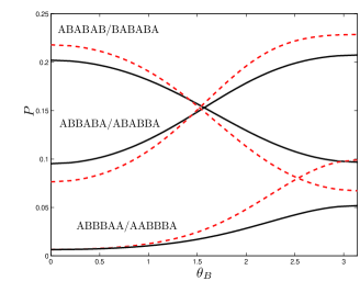
Figure 2: (Color online) Same as in Fig. 1d) but for a balanced six-body case where the $A$ particles are fermions ($\theta_{A}=\pi$) assuming an external confinement that is a box (solid lines) or a harmonic trap (dashed lines). The configurations as indicated above each set of lines. For simplicity we show only the configurations with the largest probabilities.

III Balanced systems

In Fig. 1 we show the $N=4$ case with two $A$ and two $B$ particles. Panels a), b), and c) show the slopes of the energy around $1/g=0$ as the statistics changes from Fermi-Fermi (FF) a), across Bose-Fermi (BF) b), and onto the Bose-Bose (BB) mixture case in c). Notice the totally antisymmetric state in a) which is the horizontal line and corresponds to $a_{k}=1$ for all orderings. It is only a solution in the FF case. The slopes have a distinct evolution with statistics which could in principle be observed by energy measurements in strongly interacting systems. Fig. 1 assumes a box trap but only minute quantitative changes occurs if one uses harmonic confinement. There has been a lot of recent interest in strongly interacting Fermi-Fermi harshman2012 ; brouzos2013 ; gharashi2013 ; sowinski2013 ; vol2013 ; cui2014 ; lindgren2014 ; deuret2014 and Bose-Bose mixtures zollner2008 ; hao2009 ; zinner2013 ; garcia2013 , and extended focus on the spatial configuration that such systems display for strong interactions. In Fig. 1d) we present the exact results for the ground state configurations in the limit $1/g\to 0$. For the FF mixture we see a dominant antiferromagnetic $ABAB/BABA$ configuration, while the BF case has $ABBA$ as the most probable. Finally as we go to the BB limit, the state originally proposed by Girardeau girardeau1960 becomes the exact ground state.

The generalized Girardeau type state proposed in Ref. girar2007, has a completely mixed density profile (identical to perfect fermionization of four particles) and has been shown to agree rather well with a wave function inspired by a combination of the Bethe ansatz for homogeneous space and the single-particle solutions of the particular trap fang2011 . This is a kind of hybrid solution of the trapped problem. Using our exact solutions in the strongly interacting regime one may easily check that the generalized Girardeau state is a linear combination of the eigenstates with slopes shown in Fig 1a (with coefficients that depend on the geometry of the trap). It is therefore not connected to eigenstates for large but finite interaction strengths and thus of little experimental relevance. The numerical Density Matrix Renormalization Group (DMRG) results in Ref. fang2011, seems to agree with a mixed state for very large interaction strengths which hints at an underlying issue with applying DMRG to strongly repulsive particles. It is intrinsically variational and will therefore have great difficulties with the (quasi)-degenerate many-body spectrum for strong interactions unless one uses exact solutions as a guide here. However, we notice that for large but not extreme values of the repulsive coupling strength Ref. fang2011, does indeed find the demixed ground state that is perfectly consistent with the exact result presented here.

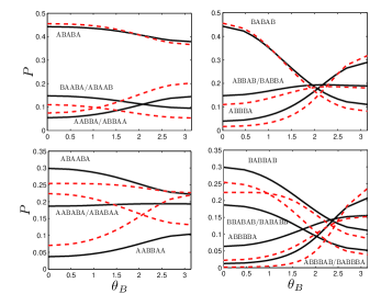
Figure 3: (Color online) Imbalanced five- (upper row) and six-body (low row) systems. All $A$ particles are fermions ($\theta_{A}=0$). The configurations follow the lines in the $\theta_{B}=0$ limit (left-hand side) from top to bottom. Solid lines are for box and dashed lines for harmonic trapping. As in Fig. 2 we show only the dominant configurations.

For larger systems the story is similar as we show in Fig. 2 with the antiferromagnetic dominance being taken over by mixed configurations as one goes from FF to BF limits. Note that we only show the configurations carrying the largest part of the total probability. We omit the results as $\theta_{A}\to\pi$ (BB limit) as they are similar to the four-body case in Fig. 1d). However, in Fig. 2 we show results for both a box and a harmonic trap which indeed demonstrates that the trap can have decisive influence on system configuration for $1/g\to 0$ both quantitatively and qualitatively. In particular, mixed configurations dominate the antiferromagnet in the BF limit for harmonic but not for box traps. This shows how trap engineering can become state engineering as first discussed in Ref. vol2013, .

IV Imbalanced systems

We now explore the interplay of statistics and imbalanced in our strongly interacting mixed systems. The two upper panels in Fig. 3 show the cases with three (left) and two (right) fermions ($A$) mixed with anyons ($B$). Again the FF limit is clearly antiferromagnetic, while in the BF limit it depends on which particle is in majority. With three $B$ particles, the BF system is dominated by the (phase separated) $ABBBA$ configuration, while with only two $B$ particles the system remains mainly antiferromagnetically ordered ($ABABA$). The differences due to the box or harmonic trap are merely quantitative in this case. In contrast, for the six-body systems in the two lower panels of Fig. 3, we do see some qualitative changes with external trap, where a harmonic trap enhances the configuration $AABBAA$ in the BF limit (lower left panel). Similarly for the lower right panel, we see enhancement of the phase separated $ABBBBA$ and $ABBBAB/BABBBA$ configurations, and again some qualitative dependence on the trap. We conclude that the tendency for phase separation for larger systems in the BF limit discussed in the introduction seems to be there but that we identify a crucial dependence on the confinement which makes the local density approximation questionable for smaller systems. An outstanding problem is to extrapolate the results obtained here to larger system sizes and match the few- and many-body limits.

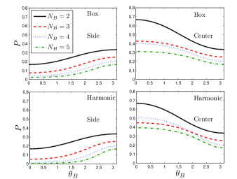
Figure 4: (Color online) Probabilities to find an impurity on the side (left column) or in the middle (right column) of an anyonic system with up to five anyons as function of statistical parameter, $\theta_{B}$. The upper row is for a box and the lower row for a harmonic trap. The middle is defined as either the single (for even $N_{B}$) or the two equivalent central positions (for odd $N_{B}$). For $\theta_{B}=\pi$ all configurations have equal probability (BB regime).

V Probing statistics with an impurity

Finally, we address the case of a single impurity that is strongly interacting with a number of anyons, $N_{B}$. As discussed above the statistic of the anyons will in general influence the energy spectrum and the configurations in the system. Measuring the ’fan’ of states shown in Fig. 1 could therefore provide insights into the statistics by comparing to the theoretical prediction given the trap shape and the number of particles. The dependence of the slopes on statistics has also been identified within the Bethe ansatz approach for single-component anyons batchelor2006b .

A different approach which can access more information about the system is to use tunneling experiments as done recently for an FF mixture zurn2012 . In the limit $1/g\to 0$ where the particles become impenetrable, one can use a simple picture when opening the trap by lowering the trap on one side zurn2012 . Here we may assume that only the particle located immediately next to the lowered barrier can tunnel. The probability that this is the impurity can then be approximated by the configurational probabilities that we have discussed above. In the left panels of Fig. 4 we show this probability for different $\theta_{B}$ in a box (upper) or harmonic (lower) trap. We see clear variation with $\theta_{B}$ and with $N_{B}$ which implies that this could be used to detect the statistics of 1D anyonic systems. While the precise way in which the trap is lowered to allow for tunneling is except to have a minor quantitative effect, we do not except qualitative differences. Alternatively, it may be possible to use single site/single atom resolution quantum gas miscroscopy bakr2009 ; sherson2010 to probe the 1D system locally simon2011 ; cheneau2012 ; fukuhara2013 . Here one can probe the probability of finding the impurity in the center of the trap which is also very sensitive to statistics as shown on the right-hand panels in Fig. 4. While the experiments cited here have an optical lattice on top of the external confinement, this will not qualitatively change our predictions. It may change the geometric factors from the confinement which can be computed using the formulas presented in Ref. vol2013, .

Appendix A Illustration of the solution technique

We now go through the simple example of three particles where two are anyons in order to illustrate the differences that arise from generalized statistics. We will be very brief and refer the interested reader to seek further details in Ref. vol2013, . To solve the problem in the limit where $1/g\to 0$ we start from the totally antisymmtric wave function, $\Psi_{A}$, which is zero whenever any of the three particles overlap in space. We work exclusively with the ground state but the technique applies to excited states as well. The coordinate space for the three particles is illustrated in Fig. 5 where $A$ are anyons with statistical parameter $\theta$, while $B$ is of a different kind (an impurity).

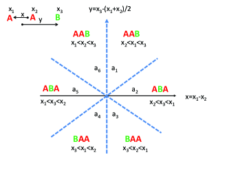
Figure 5: (Color online) Schematic of the coordinate space for the three-body problem where the $A$ particles are anyons with statistical parameter $\theta$ while single the $B$ particle can be considered an impurity.

The most general wave function with the correct boundary condition is found by taking $\Psi_{A}$ with a different coefficient, $a_{i}$, in the six regions in Fig. 5. This basis is complete and we may expand the solutions in the limit $1/g\to 0$ in this basis. As shown in Fig. 1 of the main text all solutions are degenerate in energy when $1/g=0$. We now use the fact that as $1/g\to 0$, the ground state (for $g>0$) has the maximum slope of the energy as a function of $g$. Using linear perturbation theory in $1/g$ or the Hellmann-Feynman theorem, we have $E=E_{0}-K/g$ where

$$K=\lim_{g\to\infty}\,g^{2}\frac{\sum_{i>j}\int|\Psi|^{2}\delta(x_{i}-x_{j})\prod_{k=1}^{3}dx_{k}}{\langle\Psi|\Psi\rangle}.$$ (4)

The full wave function, $\Psi$, is a function of $x_{1},x_{2},x_{3}$ and consists of the six pieces $a_{i}\Psi_{F}$ in Fig. 5. The sum, $\sum_{i>j}$, runs over all pairs according to the Hamiltonian in Eq. (1) of the main text. $\langle\Psi|\Psi\rangle$ is the normalization integral. We now eliminate $g$ by using the zero-range boundary condition

$$-\frac{1}{2g}\left[\frac{\partial\Psi}{\partial x_{+}}-\frac{\partial\Psi}{\partial x_{-}}\right]=\Psi,$$ (5)

where $x_{\pm}=\pm(x_{i}-x_{j})$.

After some calculations along the lines described in Ref. vol2013, , the expression for $K$ becomes

$$K=K_{0}\frac{(a_{1}-a_{2})^{2}+(a_{2}-a_{3})^{2}+(a_{1}^{2}+a_{3}^{2})|1-e^{-i\theta}|}{a_{1}^{2}+a_{2}^{2}+a_{3}^{2}},$$ (6)

where $K_{0}$ is a geometric factor that depends on the trapping potential and the coefficients, $a_{i}$, are real numbers. Notice that for larger systems there are more than one of these factors in the result vol2013 , but for three-body systems it can be taken outside for the parity invariant box and harmonic potentials we work with here. By variation of $K$ with respect to $a_{1}$, $a_{2}$, and $a_{3}$, one can obtain the eigenstates that are adiabatically connected to the eigenstate for large but finite $g$ as well as the slope of the energy to linear order in $1/g$.

As discussed, the decisive quantity that determines the wave functions that are adiabatically connected eigenstates in the limit $1/g=0$ is the slope of the energy, $K$. If we describe the anyons as strictly hard core particles this means they are to be regarded as ideal fermions and will make no contribution to $K$. This reduces the problem to that of two identical fermions and an impurity, and this is true no matter what value the anyonic exchange parameter, $\theta$, takes. In turn one would not be able to recover the correct Bose-Fermi mixture limit discussed in detail for the four-body system in the main text. This implies that one needs to consider the anyons when calculating the energies even in the ’hard core’ limit $1/g\to 0$ in order to have a model that matches the behavior in the known limiting cases where $\theta=0$ or $\theta=\pi$. Our approach is therefore closely related to the work using the Bethe ansatz in Refs. batchelor2006, ; batchelor2006b, , and we also obtain a strong coupling expansion of the energy which depends on $\theta$ (see Eq. (10) of Ref. batchelor2006b ). However, our formalism goes beyond the Bethe ansatz in being able to handle arbitrary confining geometries without resorting to the local density approximation.

References

- (1) J. Leinaas and J. Myrheim, Nuovo Cimento B 37, 1 (1977).
- (2) F. Wilczek, Phys. Rev. Lett. 48, 1144 (1982).
- (3) G. A. Goldin, R. Menikoff, and D. H. Sharp, J. Math. Phys. 22, 1664 (1981).
- (4) J. K. Pachos: Topoloical Quantum Computation, (Cambridge University Press, New York, 2012).
- (5) C. Nayak, S. H. Simon, A. Stern, M. Freedman, and S. Das Sarma, Rev. Mod. Phys. 80, 1083 (2008).
- (6) F. D. M. Haldane, Phys. Rev. Lett. 67, 937 (1991).
- (7) D. Alonso and S. R. Jain, Phys. Lett. B 387, 812 (1996).
- (8) S. R. Jain and D. Alonso, J. Phys. A: Math. Gen. 30, 4993 (1997).
- (9) F. Calogero, J. Math. Phys. 10, 2191 (1969); ibid. 10, 2197 (1969); ibid. 12, 419 (1971).
- (10) B. Sutherland, J. Math. Phys. 12, 246 (1971); ibid. 12, 251 (1971); Phys. Rev. A 4, 2019 (1971); ibid. 5, 1371 (1972).
- (11) A. P. Polychronakos, Nucl. Phys. B 324, 597 (1989).
- (12) G. Auberson, S. R. Jain, and A. Khare, Phys. Lett. B 267, 292 (2000); J. Phys. A: Math. Gen. 34, 695 (2001).
- (13) J. X. Zhu and Z. D. Wang, Phys. Rev. A 53, 600 (1996).
- (14) A. Kundu, Phys. Rev. Lett. 83, 1275 (1999).
- (15) M. T. Batchelor, X. W. Guan, and N. Oelkers, Phys. Rev. Lett. 96, 210402 (2006).
- (16) M. D. Girardeau, Phys. Rev. Lett. 97, 100402 (2006).
- (17) D. V. Averin and J. A. Nesteroff, Phys. Rev. Lett. 99, 096801 (2007).
- (18) A. Feiguin et al., Phys. Rev. Lett. 98, 160409 (2007).
- (19) O. I. Pâtu, V. E. Korepin, and D. V. Averin, J. Phys. A: Math. Theor. 40, 14963 (2007); ibid 41, 145006 (2008); ibid 41, 255205 (2008); ibid 42, 275207 (2009); ibid 43, 115204 (2010); Europhys. Lett. 86, 40001 (2009); ibid 87, 60006 (2009).
- (20) S. Trebst et al., Phys. Rev. Lett. 101, 050401 (2008).
- (21) A. del Campo, Phys. Rev. A 78, 045602 (2008).
- (22) L. Fidkowski, G. Refael, N. Bonesteel, and J. Moore, Phys. Rev. B 78, 224204 (2008).
- (23) M. Greiter, Phys. Rev. B 79, 064409 (2009).
- (24) R. Santachiara and P. Calabrese, J. Stat. Mech. 2008, P06005 (2008).
- (25) B. Bellazzini, P. Calabrese, and M. Mintchev, Phys. Rev. B 79, 085122 (2009).
- (26) R. A. Santos, F. N. C. Paraan, and V. E. Korepin, Phys. Rev. B 86, 045123 (2012).
- (27) B. Paredes, P. Fedichev, J. I. Cirac, and P. Zoller, Phys. Rev. Lett. 87, 010402 (2001).
- (28) M. Aguado, G. K. Brennen, F. Verstraete, and J. I. Cirac, Phys. Rev. Lett. 101, 260501 (2008).
- (29) L. Jiang et al., Nat. Phys. 4, 482 (2008).
- (30) T. Keilmann, S. Lanzmich, I. McCullosh, and M. Roncaglia, Nat. Commun. 2, 361 (2011).
- (31) F. Serwane et al., Science 332, 336 (2011).
- (32) A. Wenz et al., Science 342, 457 (2013).
- (33) J. Pellegrino et al., Phys. Rev. Lett. 113, 133602 (2014).
- (34) F. Nogrette et al., Phys. Rev. X 4, 021034 (2014).
- (35) K. K. Das, Phys. Rev. Lett. 90, 170403 (2003).
- (36) M. A. Cazalilla and A F. Ho, Phys. Rev. Lett. 91, 150403 (2003).
- (37) A. Imambekov and E. Demler, Phys. Rev. A 73, 021602(R) (2006).
- (38) B. Fang et al., Phys. Rev. A 84, 023626 (2011).
- (39) H. Wang, Y. Hao, and Y. Zhang, Phys. Rev. A 85, 053630 (2012).
- (40) A. G. Volosniev et al., Nature Commun. 5, 5300 (2014).
- (41) T. Cheon and T. Shigehara, Phys. Rev. Lett. 82, 2536 (1999).
- (42) M. D. Girardeau and M. Olshanii, Phys. Rev. A 70, 023608 (2004).
- (43) M. D. Girardeau, Phys. Rev. A 82, 011607(R) (2010).
- (44) L. W. Tonks, Phys. Rev. 50, 955 (1936).
- (45) M. D. Girardeau, J. Math. Phys. 1, 516 (1960).
- (46) M. T. Batchelor and X.-W. Guan, Phys. Rev. B 74, 195121 (2006).
- (47) N. T. Zinner et al., Europhys. Lett. 107, 60003 (2014).
- (48) N. Harshman, Phys. Rev. A 86, 052122 (2012); Phys. Rev. A 89, 033633 (2014).
- (49) I. Brouzos and P. Schmelcher, Phys. Rev. A 87, 023605 (2013).
- (50) S. E. Gharashi and D. Blume, Phys. Rev. Lett. 111, 045302 (2013).
- (51) T. Sowiński, T. Grass, O. Dutta, and M. Lewenstein, Phys. Rev. A 88, 033607 (2013).
- (52) X. Cui and T.-L. Ho, Phys. Rev. A 89, 023611 (2014).
- (53) E. J. Lindgren, J. Rotureau, C. Forssén, A. G. Volosniev, and N. T. Zinner, New J. Phys. 16, 063003 (2014).
- (54) F. Deuretzbacher et al., Phys. Rev. A 90, 013611 (2014).
- (55) S. Zöllner, H.-D. Meyer, and P. Schmelcher, Phys. Rev. A 78, 013629 (2008).
- (56) Y. J. Hao and S. Chen, Phys. Rev. A 80, 043608 (2009); Eur. Phys. J. D 51, 261 (2009).
- (57) M. A. Garcia-March et al., Phys. Rev. A 88, 063604 (2013); New J. Phys. 16 103004 (2014).
- (58) M. D. Girardeau and A. Minguzzi, Phys. Rev. Lett. 99, 230402 (2007).
- (59) G. Zürn et al., Phys. Rev. Lett. 108, 075303 (2012); Phys. Rev. Lett. 111, 175302 (2013).
- (60) W. S. Bakr, J. I. Gillen, A. Peng, S. Fölling, and M. Greiner, Nature 462, 74 (2009).
- (61) J. F. Sherson et al., Nature 467, 68 (2010).
- (62) J. Simon et al., Nature 472, 307 (2011).
- (63) M. Cheneau et al., Nature 481, 484 (2012).
- (64) T. Fukuhara et al., Nature Phys. 9, 235 (2013).