Impurity electrons in narrow electric field-biased armchair graphene nanoribbons

Abstract

We present an analytical investigation of the quasi-Coulomb impurity states in a narrow gapped armchair graphene nanoribbon (GNR) in the presence of a uniform external electric field directed parallel to the ribbon axis. The effect of the ribbon confinement is taken to be much greater than that of the impurity electric field, which in turn considerably exceeds the external electric field. Under these conditions we employ the adiabatic approximation assuming that the motion parallel (”slow”) and perpendicular (”fast”) to the ribbon axis are separated adiabatically. In the approximation of the isolated size-quantized subbands induced by the ”fast” motion the complex energies of the impurity electron are calculated in explicit form. The real and imaginary parts of these energies determine the binding energy and width of the quasi-discrete state, respectively. The energy width increases with increasing the electric field and ribbon width. The latter forms the background of the mechanism of dimensional ionization. The S-matrix - the basic tool of study of the transport problems can be trivially derived from the phases of the wave functions of the continuous spectrum presented in explicit form. In the double-subband approximation we calculate the complete widths of the impurity states caused by the combined effect of the electric field and the Fano resonant coupling between the impurity states of the discrete and continuous spectra associated with the ground and first excited size-quantized subbands. Our analytical results are shown to be in agreement with those obtained by other theoretical approaches. Estimates of the expected experimental values for the typically employed GNRs show that for weak electric field the impurity quasi-discrete states remain sufficiently stable to be observed in corresponding experiment, while relatively strong field unlock the captured electrons to further restore their contribution to the transport.

I Introduction

Experimental and theoretical studies of the transport, electronic and optical properties of the armchair graphene nanoribbon (GNR) have attracted much attention in recent years. One of the reason for this is that the GNRs used as the interconnects in graphene-based nanoelectronic and as the basic elements in the logic transistors could provide ultrahigh carrier mobility between the unbounded gapless 2D graphene monolayers. However, the opened band gap in GNR reduces considerably the mobility of the carriers Wang13 . Additional inevitable difficulties come from the fact that in contrast to gapless graphene monolayers, in which the bound impurity states are forbidden Bis ; Nov ; Per ; Shyt ; Shyt1 in gapped graphene Nov ; Peder ; Gupta08 and quasi 1D GNR monschm12 the bound impurity states can be realized. The binding energies $E^{(b)}$ of the impurity electrons in the GNR of width $1~{}\mbox{nm}$ reach the considerable amount of the order of $E^{(b)}\simeq 1\mbox{~{}}{eV}$. In addition, it was shown monschm12 that impurity electrons, possessing energies close to the Breit-Wigner meta-stable resonances, contribute negligibly little to the conductance. Clearly, the impurity centres suppress strongly the mobility of the GNRs. Of course the binding effect of the impurity centres could be reduced by the technologically involved procedure of the improvent of the sample standard Wang13 . Nevertheless the less elaborate mechanism of the liberation of the carriers captured by the impurities is a much more immediate demand at the present time. The process of the ionization by an external electric field can be used as an instrument for the release of the blocked carriers.

Besides, the quasi-1D structures, in particular the bulk semiconductors subject to strong magnetic fields ZhMak , quantum wires (QWRs) monschm09 and armchair GNRs monschm12 are favorable for the formation of both the strictly discrete and meta-stable (Fano resonances) Fano impurity and exciton states adjacent to the ground and excited size-quantized energy levels, respectively. The latter are caused by the confinement effect associated with the magnetic field in bulk semiconductors and the boundaries of the QWRs and GNRs. The nature of the Fano resonances comes from the inter subband coupling between the discrete and low-lying continuous Rydberg states. With emergence of the electric field only one channel of the ionization is opened for the ground series of the Rydberg discrete states, while the excited meta-stable states decay into two channels: the autoionization channel, open due to the inter-subband Fano coupling, and the channel of the electric field ionization, related to the under-barrier tunneling (Fig. 1). The interaction of these two channels of the ionization is of immediate interest.

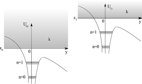
Figure 1: (color online). The combined potential $U_{NN}(y)=V_{NN}(y)-eFy$, formed by the impurity potential $V_{NN}(y)$ (9) and electric field $F$ adjacent to the ground and first excited size-quantized energy levels $\varepsilon_{N}$ (5) with $N=0,1$, respectively. The continuous and discrete Rydberg states are labeled by the indexes $(k)$ and $n=0$ (ground state) and $n=1$ (first excited state), respectively.

It is clear that the problem of the impurity states in the armchair GNR in the presence of a longitudinal electric field directed parallel to the GNR axis is important on account of two aspects: (i) its considerable interest in the context of basic research, and (ii) possible nano-electronic applications.

Narrow GNRs of several nanometers width are the best candidates among the other 1D structures for fundamental studies. The binding energies of the impurity electron in GNR exceed those in the corresponding semiconductor structures by a factor of about $10^{2}$ that in particular manifests itself in the strong electric fields, providing the complete ionization of the impurity states in GNR. GNRs seem to be a unique structure in which both channels of the auto- and electric field ionization are opened. The process of electric field ionization transforms the strictly bound and the Fano resonant states into states of transporting carriers that in turn improve the conductance properties of the GNRs and of the nano-electronic devices into which these ribbons are incorporated. The finite lifetime of the quasi-discrete impurity states associated with the two-channel ionization should be taken into account in the practical use of the GNRs exposed to the electric field.

There are two comments in order. First, the theoretical approaches to this problem are mostly based on numerical calculations (density functional theory and Bethe-Salpiter equation Yang07 , nonorthogonal tight-binding model Jia , tight-binding scheme and Hartree-Fock approximation Mohamm ) requiring significant computational efforts. Only a few recent works elaborate on analytical methods. In Ref. monschm12 the bound and quasi-discrete impurity states in the armchair GNR have been studied by solving the Dirac equation for a massless neutrino. Ratnikov and Silin RatSil empirically extended to the GNR the model earlier developed for the semiconductor QWR Bab , and calculated the excitonic energy levels by the variational method and their red shift induced by the electric field. Second, to our knowledge analytical results based on the Dirac equation adequately describing the impurity electrons in GNRs subject to external electric field are not present in the literature. Thus an analytical approach to the problem of the impurity states in biased armchair GNR is desirable. Particularly it renders the basic physics transparent and governs the electronic, optical and transport properties of the graphene based devices.

In the present work we develop an analytical approach to the problem of the impurity state in the narrow armchair GNR in the presence of an external electric field directed parallel to the ribbon axis. The Coulomb impurity attraction is taken to be much weaker than the influence of the ribbon confinement and much stronger than the effect of the electric field. The impurity centre can be positioned anywhere within the GNR. The 2D Dirac equation for the massless neutrino subject to the Coulomb and external uniform electric field is solved in the adiabatic approximation. This approximation implies the transverse motion of the electron governed by the ribbon confinement to be much faster than the longitudinal motion controlled by the impurity and external electric field. Our approach is based on the matching of the wave functions in the intermediate regions. The latter separates the impurity interaction from the electric field interaction dominated regimes. In the approximation of the isolated size-quantized subbands the binding energies and widths of the quasi-discrete states as a function of the ribbon width, position of the impurity and the electric field are calculated in explicit form. Also, the phases of the functions of the continuous spectrum specifying the S-matrix are derived. In the double-subband approximation the total widths of the first excited Rydberg series of impurity states, associated with the ionization effect of the electric field and inter-subband Fano coupling are calculated. Also the capturing of the electron by the impurity potential for the lifetime determined by the electric field is explored. Numerical estimates made for realistic GNR show that for narrow ribbons the impurity states in the presence of a weak electric field remain quite stable which is to be proven experimentally, while significantly strong field could unlock the captured electrons. The aim of this work is to clarify the ionization mechanism of the release of the strictly bound and quasi-bound impurity electrons yielding the increase of the mobility of the carriers in the GNR.

This work is organized as follows. In Section 2 the general analytical approach is described. The complex quasi-discrete energy levels dictating the binding energies and energy widths caused by the electric field along with the phases of the wave functions of the continuous states are calculated in the single-subband approximation in Section 3. The combined effect of the autoionization of the Fano resonant states and their ionization by the electric field is under consideration in Section 4. In Section 5 we discuss the obtained results and estimate the expected experimental values. Section 6 contains the conclusions.

II General approach

We consider a ribbon of width $d$ placed in the $x-y$ plane and bounded by the lines $x=\pm d/2.$ The impurity centre of charge $Z$ is shifted from the mid-point of the ribbon $x=0$ by the distance $-d/2\leq x_{0}\leq d/2.$ The equation describing the impurity electron at a position $\vec{\rho}=(x,y)$ subject to the external uniform electric field $\vec{F}\parallel-\vec{e}_{y}$ possesses the form of a Dirac equation

$$\hat{{\rm H}}(\hat{\vec{k}},\vec{\rho})\vec{\Psi}(\vec{\rho})=E\vec{\Psi}(\vec{\rho});\qquad\hat{\vec{k}}=-i\vec{\nabla};$$ (1)

where the Hamiltonian $\hat{{\rm H}}$ relevant to the inequivalent Dirac points
$\vec{K}^{(+,-)}(\pm K,0)~{};\,(K=4\pi/3a_{0},~{}a_{0}=2.46~{}{\rm{\AA}}$ is the graphene lattice constant) is given by monschm12 ; Brey

$$\hat{{\rm H}}=p\left[\left(\begin{array}[]{cc}-\sigma_{x}\hat{k}_{x}&0\\ 0&\sigma_{x}\hat{k}_{x}\\ \end{array}\right)+\left(\begin{array}[]{cc}-\sigma_{y}\hat{k}_{y}&0\\ 0&-\sigma_{y}\hat{k}_{y}\end{array}\right)\right]+\left[V(\vec{\rho})-eFy\right]\hat{{\rm I}};$$

containing the Pauli matrixes $\sigma_{x,y}$, the graphene parameter $p=\hbar v_{F};\,(v_{F}=10^{6}~{}\mbox{m/s})$, the unit matrix $\hat{{\rm I}}$ and the 2D Coulomb impurity potential

$$V(\vec{\rho})=-\frac{\beta}{\sqrt{(x-x_{0})^{2}+y^{2}}}~{};\qquad\beta=\frac{Ze^{2}}{4\pi\epsilon_{0}\epsilon_{\mbox{eff}}}~{};$$ (2)

Here $\epsilon_{\mbox{eff}}=\frac{1}{2}(1+\epsilon+\pi q_{0})$ is the effective dielectric constant determined by the static dielectric constant $\epsilon$ of the substrate Nov ; hwang and by the parameter $q_{0}=\frac{e^{2}}{4\pi\epsilon_{0}\hbar v_{F}}\simeq 2.2.$

The envelope wave function four-vector $\vec{\Psi}$

$$\vec{\Psi}(\vec{\rho})=\begin{array}[]{c}\begin{Bmatrix}\psi_{A}^{(+)}\\ 0\\ \psi_{A}^{(-)}\\ 0\end{Bmatrix}\end{array}+\begin{array}[]{c}\begin{Bmatrix}0\\ \psi_{B}^{(+)}\\ 0\\ \psi_{B}^{(-)}\\ \end{Bmatrix}\end{array}$$

consists of the wave functions $\psi^{(+,-)}_{A,B}(\vec{\rho})$ describing the electron states in the sublattices $A$ and $B$ of graphene in the vicinity of the Dirac points $\vec{K}^{(+,-)}$, respectively. The boundary conditions require the total wave function to vanish at both edges for each sublattice Castro

$$e^{{\rm i}Kx}\psi_{j}^{(+)}(\vec{\rho})+e^{-{\rm i}Kx}\psi_{j}^{(-)}(\vec{\rho})=0~{}\mbox{at}\,x=\pm\frac{d}{2},~{}\mbox{for}~{}j=\mbox{A,B}$$ (3)

By solving eq. (1) the components $\psi^{(+,-)}_{A,B}$ of the total wave vector $\vec{\Psi}(\vec{\rho})$ subject to the boundary conditions (3) can be found.

Following the procedure presented in details in Ref. monschm12 we expand the wave functions $\psi^{(+,-)}_{A,B}$ in a series

$$\psi_{j}^{(+,-)}(\vec{\rho})=\Sigma_{N}u_{Nj}(y)\varphi_{Nj}^{(+,-)}(x),~{}j=\mbox{A,B},$$

in which

$$-\varphi_{NA}^{(+)} = \varphi_{NA}^{(-)*}=\varphi_{NB}^{(+)}=-\varphi_{NB}^{(-)*}=\varphi_{N0};$$

$$\varphi_{N0}(x) = \frac{1}{\sqrt{2d}}\exp\left\{{\rm i}\left[x\frac{\pi}{d}(N-\tilde{\sigma})-\frac{\pi}{2}\left(N+\left[\frac{Kd}{\pi}\right]\right)\right]\right\}$$ (4)

are the components of the orthonormal $N$-vector wave function relevant to the transverse confined $x$-motion of the free electron with the size-quantized energies

$$\varepsilon_{N}=|N-\tilde{\sigma}|\frac{\pi p}{d};~{}N=0,\pm 1,\pm 2,\ldots~{};\quad\tilde{\sigma}=\frac{Kd}{\pi}-\left[\frac{Kd}{\pi}\right].$$ (5)

Below for estimates we take the GNRs of the family $\tilde{\sigma}=1/3$ providing along with $\tilde{\sigma}=2/3$ the semiconductor-like gapped structure, leaving aside $\tilde{\sigma}=0$, corresponding to the metallic-like gapless ribbon. This leads to the set of the equations for the coefficients

$$v_{N}^{(1,2)}=\frac{1}{\sqrt{2}}(u_{NB}\pm u_{NA});$$

$$\left.\begin{array}[]{c}\frac{dv_{N}^{(1)}(y)}{dy}-\frac{1}{p}\left(E+\varepsilon_{N}-V_{NN}(y)+eFy\right)v_{N}^{(2)}(y)+\frac{1}{p}\sum_{N^{\prime}\neq N}V_{N^{\prime}N}(y)v_{N^{\prime}}^{(2)}(y)=0~{};\\ \frac{dv_{N}^{(2)}(y)}{dy}+\frac{1}{p}\left(E-\varepsilon_{N}-V_{NN}(y)+eFy\right)v_{N}^{(1)}(y)-\frac{1}{p}\sum_{N^{\prime}\neq N}V_{N^{\prime}N}(y)v_{N^{\prime}}^{(1)}(y)=0~{};\end{array}\right\}$$ (8)

$$V_{N^{\prime}N}(y)=\frac{1}{d}\int_{-\frac{d}{2}}^{+\frac{d}{2}}V(\vec{\rho})\cos\left[(N-N^{\prime})\pi\left(\frac{x}{d}-\frac{1}{2}\right)dx\right],$$ (9)

with eq. (2) for the potential $V(\vec{\rho})$. At $|y|\gg d$

$$V_{N^{\prime}N}(y)=-\frac{\beta}{|y|}\left[\delta_{N^{\prime}N}+O\left(\frac{d^{2}}{y^{2}}\right)\delta_{|N^{\prime}-N|(2s+1)}\right]~{};\,s=0,1,2,\ldots;$$ (10)

Below we solve the set (8) in the adiabatic approximation. The longitudinal $y$-motion, governed by the quasi-Coulomb potentials $V_{N^{\prime}N}(y)$ slightly perturbed by the electric field $F$, is assumed to be much slower than the transverse $x$-motion affected by the boundaries of the narrow ribbon.

The relevant parameters are the strength of the impurity potential scaled to that of the graphene $q$, the impurity Bohr radius $a_{0}$, the quantum number of the bound impurity state $\eta$ and the dimensionless electric field $f$, which is the external electric field $F$ scaled to the impurity electric field $F_{0}$. They are defined by

$$q=\frac{\beta}{p};\quad a_{0}=\frac{p}{Eq};\quad\eta=q\frac{E}{\sqrt{\varepsilon_{N}^{2}-E^{2}}};\quad f=\frac{F}{F_{0}};\quad F_{0}=\frac{qp}{ea_{0}^{2}};$$ (11)

The other parameters $y_{1}=2\eta^{2}a_{0}$ and $y_{2}=(\varepsilon_{N}-E)(eF)^{-1}$ - are the first and second quasi-classical turning points calculated from $\mathcal{P}(y_{1,2})=0$, where

$$\mathcal{P}(y)=\frac{1}{v_{F}}\left[\left(E+\frac{\beta}{y}+eFy\right)^{2}-\varepsilon_{N}^{2}\right]^{1/2};$$

is the quasi-classical momentum. Further we impose the conditions

$$q\ll 1$$ (12)

meaning the narrowness of the ribbon $d\ll a_{0}$ (at any rate for the low excited size-quantized $N$ subbands) i.e. the smallness of the impurity effect comparatively to that of the confinement, and

$$f\eta^{3}\ll 1$$ (13)

providing the weakness of the external electric field $F$ relatively to the impurity electric field in the state with quantum number $\eta$. Under these conditions the relationships

$$a_{0},y_{1}\ll y_{2},\,a_{0}=\frac{d}{\pi|N-\tilde{\sigma}|q},~{}y_{2}=\frac{\varepsilon_{N}q^{2}}{2\eta^{2}eF}$$

are valid.

III Single-subband approximation

At the first stage we neglect the coupling between the states associated with the subbands of different $N.$ It follows from eq. (10), that in the narrow ribbon of small width $d$ the diagonal potentials $V_{NN}$ dominate the off-diagonal terms which allows in turn allows to take $V_{N^{\prime}N}=V_{NN}\delta_{N^{\prime}N}$ and then to decompose the set (8) into independent equations with the potentials

$$V_{NN}(y)=\frac{\beta}{d}\ln\frac{\frac{4y^{2}}{d_{1}d_{2}}}{\left(1+\sqrt{1+\frac{4y^{2}}{d_{1}^{2}}}\right)\left(1+\sqrt{1+\frac{4y^{2}}{d_{2}^{2}}}\right)}=\left\{\begin{array}[]{cl}\frac{\beta}{d}\ln\frac{y^{2}}{d_{1}d_{2}}~{};&\frac{|y|}{d_{1,2}}\ll 1\\ -\frac{\beta}{|y|}~{};&\frac{|y|}{d_{1,2}}\gg 1\end{array}\right.$$ (16)

$$d_{1,2}=d\pm 2x_{0}~{};\qquad-\frac{d}{2}\leq x_{0}\leq+\frac{d}{2}~{};$$

The set (8) for $V_{N^{\prime}N}=0$ is solved by matching in the intermediate regions the two-vectors $\vec{V}_{N}=(v_{N}^{(1)},v_{N}^{(2)})$ valid in the inner region $0\leq y\ll a_{0}$, Coulomb region $d\ll y\ll y_{2}$ and in the ”electric” region $a_{0}\ll y$ monschm12 . In the inner and Coulomb regions the impurity electric field $F_{0}$ considerably exceeds the external uniform field $F$, while in the ”electric” region the potentials $V_{NN}(y)$ can be treated as a small perturbation to the effect of the field $F$.

III.1 Discrete states $E<\varepsilon_{N}$

Inner region

In this region an iteration procedure is employed. The subsequent integration of the set (8), in which we keep only diagonal potentials $V_{NN}(y)$ (16) and take arbitrary constants for the trial functions $v_{N}^{(1,2)}$, gives for the even states $\vec{V}_{N}$ in the intermediate region $d\ll y\ll a_{0}$ monschm12

$$v_{N\mbox{it}}^{(1)}(y)=\sin(Q(y)+\zeta);\quad v_{N\mbox{it}}^{(2)}(y)=\cos(Q(y)+\zeta)~{};$$ (17)

where

$$Q(y)=q\frac{y}{|y|}\left(\ln\frac{4|y|}{D}+1\right),\quad D=\sqrt{d_{1}d_{2}}\exp\left\{\frac{1}{4d}(d_{1}-d_{2})\ln\frac{d_{1}}{d_{2}}\right\}$$

and $\zeta$ is an arbitrary constant phase.

Coulomb region

In this region the wave two-vector $\vec{V}_{N\mbox{C}}$ can be written in the form

$$\vec{V}_{NC}(y)=R_{-}\vec{V}_{NC}^{(-)}(y)+R_{+}\vec{V}_{NC}^{(+)}(y)$$ (18)

where $\vec{V}_{NC}^{(+)}~{}\mbox{and}~{}\vec{V}_{NC}^{(-)}$ are the vectors increasing and decreasing, respectively at $|y|\rightarrow\infty$, and where $R_{\pm}$ are the corresponding arbitrary constants. The components determining the vector $\vec{V}_{NC}^{(-)}$, have been calculated in Ref. monschm12 in terms of the exact solutions to eqs. (8) at $V_{NN}(y)=-\beta|y|^{-1}~{}\mbox{and}~{}F=0$

$$v_{NC(-)}^{(1)}(y)=\cosh\frac{\psi}{2}\tau^{-\frac{1}{2}}\left[W_{\kappa,\mu}(\tau)+\frac{\tanh\psi}{q}W_{\kappa+1,\mu}(\tau)\right],$$ (19)

where

$$\tau=\frac{2}{\eta a_{0}}y;~{}\quad\tanh\psi=\frac{q}{\eta};\quad\kappa=\eta-\frac{1}{2};\quad\mu={\rm i}q,$$

and where $W_{\kappa,\mu}(\tau)$ is the Whittaker function having the asymptotics $\exp(-\frac{\tau}{2})$ abram . The function $v_{NC(-)}^{(2)}(y)$ can be obtained from eq. (19) by replacing $\cosh\frac{\psi}{2}~{}\mbox{by}~{}\sinh\frac{\psi}{2}~{}\mbox{and}~{}q~{}\mbox{by}~{}-q$. The wave functions $v_{NC(+)}^{(1,2)}$, corresponding to the vector $\vec{V}_{NC}^{(+)}$, are derived from the functions $v_{NC(-)}^{(1,2)}$, respectively by replacing $W_{\kappa,\mu}~{}\mbox{by}~{}M_{\kappa,\mu},~{}W_{\kappa+1,\mu}~{}\mbox{by}~{}M_{\kappa+1,\mu}~{}\mbox{and}~{}q~{}\mbox{by}~{}q(\eta+{\rm i}q)^{-1}~{}\mbox{where}~{}M_{\kappa,\mu}(\tau)$ is the Whittaker function having the asymptotics $\exp(\frac{\tau}{2})$ abram .

At $\tau\ll 1~{}\mbox{and}~{}q\ll 1$

$$v_{NC(-)}^{(1)}(y)=-\frac{1}{\eta^{2}\Gamma(-\eta)}\sin\omega(y);\quad v_{NC(-)}^{(2)}(y)=-\frac{1}{\eta^{2}\Gamma(-\eta)}\cos\omega(y);$$ (20)

$$v_{NC(+)}^{(1)}(y)=\frac{q}{\eta}\sin(q\ln\tau);\quad v_{NC(+)}^{(2)}(y)=\frac{q}{\eta}\cos(q\ln\tau);$$ (21)

where $\omega(y)=q\ln\tau+\Theta(\eta)$ with

$$\Theta(\eta)=\frac{\pi}{2}+2qC+\arg\Gamma(-\eta+{\rm i}q)-\frac{q}{2\eta}.$$ (22)

In eq. (22) $C=0.577$ is the Euler constant and $\Gamma(x)$ is the $\Gamma$-function.

At $\tau\gg 1$

$$v_{NC(-)}^{(1)}(y)=\frac{1}{\eta}\tau^{\eta}{\rm e}^{-\frac{\tau}{2}};\quad v_{NC(-)}^{(2)}(y)=-\frac{q}{2\eta}v_{NC(-)}^{(1)}(y);$$ (23)

$$\left.\begin{array}[]{c}v_{NC(+)}^{(1)}(y)=-\frac{1}{\eta}\left[\frac{{\rm e}^{-\rm i\pi\eta}}{\Gamma(\eta)}\tau^{\eta}{\rm e}^{-\frac{\tau}{2}}+\frac{1}{\Gamma(-\eta)}\tau^{-\eta}{\rm e}^{+\frac{\tau}{2}}\right];\\ v_{NC(+)}^{(2)}(y)=\frac{q}{2\eta^{2}}\left[\frac{{\rm e}^{-\rm i\pi\eta}}{\Gamma(\eta)}\tau^{\eta}{\rm e}^{-\frac{\tau}{2}}-\frac{1}{\Gamma(-\eta)}\tau^{-\eta}{\rm e}^{+\frac{\tau}{2}}\right];\end{array}\right\}$$ (26)

”Electric region”

The problem of the relativistic electron in the presence of a uniform electric field has been studied initiatively by Sauter Sauter . Using the original notations

$$\xi=\sqrt{\frac{eF}{p}}y+\xi_{0};\quad\xi_{0}=\frac{E}{\sqrt{eFp}};\quad k_{0}=\frac{\varepsilon_{N}}{\sqrt{eFp}};$$

the set (8) for the functions $v_{N\mbox{el}}^{(1,2)}$ reads

$$\left.\begin{array}[]{c}v_{N\mbox{el}}^{(1)^{\prime\prime}}(\xi)+\frac{-1+\frac{q}{(\xi-\xi_{0})^{2}}}{k_{0}+\xi+\frac{q}{\xi-\xi_{0}}}v_{N\mbox{el}}^{(1)^{\prime}}(\xi)-\left[k_{0}^{2}-\left(\xi+\frac{q}{\xi-\xi_{0}}\right)^{2}\right]v_{N\mbox{el}}^{(1)}(\xi)=0~{};\\ v_{N\mbox{el}}^{(2)}(\xi)=\frac{1}{k_{0}+\xi+\frac{q}{\xi-\xi_{0}}}v_{N\mbox{el}}^{(1)^{\prime}}(\xi)~{};\end{array}\right\}$$ (29)

Using the relationships $k_{0},~{}\xi_{0},~{}\xi\gg 1$ induced by the conditions (12) and (13) and setting

$$v^{(1)}_{N\mbox{el}}(\xi)=(\xi+k_{0})^{\frac{1}{2}}\varphi(\xi)(x)~{};$$ (30)

$$\xi=k_{0}\left[1-(2k_{0}^{4})^{-\frac{1}{3}}x\right]~{},x=(2k_{0})^{\frac{1}{3}}\sqrt{\frac{eF}{p}}(y-y_{2});\quad x\ll k_{0}^{\frac{4}{3}};$$

we obtain from eq. (29)

$$\varphi^{{}^{\prime\prime}}(x)-G(x)\varphi(x)=0~{},$$ (31)

where

$$G(x)=x-2q(2k_{0})^{-\frac{2}{3}}\frac{\xi_{0}}{k_{0}-\xi_{0}-(2k_{0})^{-\frac{1}{3}}x}.$$

Eq. (31) is solved by the method of a comparison equation Slav successfully employed in Ref. monschm09 in which the impurity and exciton in a biased quantum wire have been studied. The key point of this method is the replacements of the coefficient $G(x)$ and the function $\varphi(x)$ by others which transform eq. (31) into an exactly analytically solvable comparison equation (see Refs. Slav and monschm09 for details). The solutions to eq. (31) $\varphi_{1,2}(x)$ are written in terms of the Airy functions $Ai(S)$ and $Bi(S)$ abram

$$\varphi_{1}(x)=\frac{\left[\frac{3}{2}S(x)\right]^{\frac{1}{6}}}{G(x)^{\frac{1}{4}}}Ai\left[\left(\frac{3}{2}S(x)\right)^{\frac{2}{3}}\right]~{};\quad\varphi_{2}(x)=\frac{\left[\frac{3}{2}S(x)\right]^{\frac{1}{6}}}{G(x)^{\frac{1}{4}}}Bi\left[\left(\frac{3}{2}S(x)\right)^{\frac{2}{3}}\right]~{};$$ (32)

where

$$S(x)=\int_{0}^{x}G^{\frac{1}{2}}(x)dx.$$ (33)

At $y\ll y_{2}$ resulting in $x,S\gg 1$, the asymptotic expansions for $Ai(S)~{}\mbox{and}~{}Bi(S)$ abram in eqs. (32) give for the functions $v_{N\mbox{el}}^{(1)}$ (30) and $v_{N\mbox{el}}^{(2)}$ (29)

$$v_{N\mbox{el}}^{(1)(-)}(y) = \pi^{-\frac{1}{2}}x_{2}^{-\frac{1}{4}}\exp\left[S(y)\right]~{};~{}v_{N\mbox{el}}^{(1)(+)}(y)=\pi^{-\frac{1}{2}}x_{2}^{-\frac{1}{4}}\frac{1}{2}\exp\left[-S(y)\right]~{};$$

$$v_{N\mbox{el}}^{(2)(\mp)}(y) = \mp\frac{q^{2}}{4\eta^{2}}v_{N\mbox{el}}^{(1)(\mp)}(y)~{};\quad x_{2}=(2k_{0})^{\frac{1}{3}}\sqrt{\frac{eF}{p}}y_{2}~{};$$ (34)

where

$$S(y)=\frac{1}{3\eta^{3}f}-\frac{y}{\eta a_{0}}+\eta\ln\frac{y}{4y_{2}}.$$ (35)

The components $v_{N\mbox{el}}^{(1,2)(\pm)}$ in eqs. (III.1) determine the two-vector $\vec{V}_{N\mbox{el}}$ in the region $y\ll y_{2}$

$$\vec{V}_{N\mbox{el}}(y)=C_{0}\left[\vec{V}_{N\mbox{el}}^{(-)}(y)+{\rm i}\vec{V}_{N\mbox{el}}^{(+)}(y)\right],$$ (36)

where $C_{0}$ is an arbitrary constant. Note, that in the region $y>y_{2}$ the vector state (36) with eqs. (29), (30), (32), possesses the asymptotics of the outgoing wave

$$\vec{V}_{N\mbox{el}}(y)=C_{0}\pi^{-\frac{1}{2}}x^{-\frac{1}{4}}\exp\left\{{\rm i}\left[\frac{k_{0}^{2}}{3}\left(\frac{2eF}{\varepsilon_{N}}(y-y_{2})\right)^{\frac{3}{2}}+\frac{\pi}{4}\right]\right\}.$$

On equating in the intermediate region $d\ll y\ll a_{0}$ the two-vectors $\vec{V}_{N\mbox{it}}$ and $\vec{V}_{NC}$ (18) with the components (17) and (20), (21) for the vectors $\vec{V}_{N\mbox{it}}$ and $\vec{V}_{NC}$, respectively, we obtain

$$-R_{-}\frac{1}{\Gamma(-\eta+1)}Y(\eta)+R_{+}=0$$ (37)

with

$$Y(\eta)=\frac{1}{q}\left[\Theta(\eta)-q\left(\ln\frac{2\eta a_{0}}{D}+1\right)-\zeta\right].$$ (38)

Taking in eq.(22) $\Theta(\eta)~{}\mbox{for}~{}\zeta=\pi/2~{}\mbox{and}~{}q\ll 1$, the function $Y(\eta)$ reads in an explicit form

$$Y = q^{-1}\left[\arctan\left(\frac{1}{z}-\frac{n}{q}\right)^{-1}-\arctan\frac{z}{2}\right]+\ln z+\psi\left(1+\frac{q}{z}\right)+X_{N}~{};$$ (39)

$$X_{N} = \ln\left\{\frac{|N-\tilde{\sigma}|\pi}{2}\sqrt{1-s^{2}}\exp\left[\frac{s}{2}\ln\frac{1+s}{1-s}\right]\right\}+2C-1~{};$$

In eq. (39) $z=q/\eta~{},s=2x_{0}/d~{},\quad\eta=n+\delta_{Nn}~{},\quad n=0,1,2\ldots,$ and $\psi(x)=\Gamma^{\prime}(x)/\Gamma(x)$ is the logarithmic derivative of the $\Gamma(x)$-function. In an effort to make the further results more readable and transparent, we utilize the logarithmic approximation $|q\ln q|\ll 1~{}(z\ll 1)$ , which transforms eq. (39) into

$$Y(\eta)=\frac{1}{\eta-n}-\frac{1}{2\eta}+\ln q-\ln\eta+\psi\left(1+\eta\right)+X_{N}~{};~{}n=0,1,2\ldots$$ (40)

for the $Y$ function and for its derivative we obtain

$$\frac{\partial Y}{\partial\eta}=-\frac{1}{(\eta-n)^{2}}+\frac{1}{2\eta^{2}}~{},\quad n=0,1,2\ldots.$$ (41)

A comparison in the other intermediate region $a_{0}\ll y\ll y_{2}$ the Coulomb vector $\vec{V}_{NC}$ (18), (20), (21) and ”electric” vector $\vec{V}_{N\mbox{el}}$ (36), (III.1) yield

$$\left.\begin{array}[]{c}-R_{-}+R_{+}\frac{(-1)^{\eta}}{\Gamma(\eta)}+C_{0}\pi^{-\frac{1}{2}}x_{2}^{-\frac{1}{4}}\eta\Phi_{\eta}^{-1}=0~{};\\ R_{+}\frac{1}{\Gamma(-\eta)}+C_{0}\pi^{-\frac{1}{2}}x_{2}^{-\frac{1}{4}}{\rm i}\frac{\eta}{2}\Phi_{\eta}=0~{};\end{array}\right\}$$ (44)

where

$$\Phi_{\eta}=\exp\left(-\frac{1}{3\eta^{3}f}+\eta\ln\frac{4}{\eta^{3}f}\right)~{},\Phi_{\eta}\ll 1.$$ (45)

On solving the set (37), (44) by the determinantal method we arrive at the equation for the complex quantum numbers $\eta$ and complex energies $E$

$$-\frac{1}{2}\Gamma(1-\eta)\left[\frac{\Gamma(-\eta)}{Y(\eta)}+\frac{(-1)^{\eta}}{\Gamma(1+\eta)}\right]\Phi_{\eta}^{2}+{\rm i}=0.$$ (46)

The quantum numbers $\eta_{Nn}=n+\delta_{Nn}~{},n=0,1,2\ldots$ of the strictly discrete states related to the zero electric field $F=\Phi_{\eta}=0$ can be found from equation $Y(\eta)=0$ with eq. (40) for the $Y$ function. On expanding this function in eq. (46) in the vicinity of the quantum numbers $\eta_{Nn}$ and taking into account the derivative (41) we calculate the complex quantum numbers $\eta(E)$ which in turn determine the quasi-discrete energy levels

$$E_{Nn}=\varepsilon_{N}\left(1-\frac{q^{2}}{2\eta^{2}}\right)-{\rm i}\frac{\Gamma_{Nn}^{(\mbox{el})}}{2}~{};$$ (47)

where the energy width

$$\Gamma_{Nn}^{(\mbox{el})}=\left\{\begin{array}[]{cl}2\delta_{N0}^{-2}\varepsilon_{N}q^{2}\Phi_{0}^{2}~{};\quad n=0~{};\\ \\ (nn!)^{-2}\varepsilon_{N}q^{2}\Phi_{n}^{2}~{};\quad n=1,2,\ldots~{};\end{array}\right.$$ (51)

Replacing the vector (36) by the ”electric” vector $\vec{V}_{N\mbox{el}}$

$$\vec{V}_{N\mbox{el}}=C_{0}\left[\cos\Omega_{0}\vec{V}_{N\mbox{el}}^{(-)}(y)-\sin\Omega_{0}\vec{V}_{N\mbox{el}}^{(+)}(y)\right],$$ (52)

where $C_{0}$ and $\Omega_{0}$ are the arbitrary constant and phase, respectively, we obtain

$$\cot\Omega_{0}=\left\{-\frac{1}{2}\left[\frac{\Gamma(-\eta)}{Y}+\frac{(-1)^{\eta}}{\Gamma(1+\eta)}\right]\Gamma(1-\eta)\Phi_{\eta}^{2}\right\}^{-1}$$ (53)

The results of this subsection summarized in eqs. (47), (51), and (53) are valid under the conditions (12) as well as $|q\ln q|\ll 1$ and (13).

III.2 Continuous states $E>\varepsilon_{N}$

Inner region

As above the wave functions, corresponding to the inner region are given by eqs. (17).

Coulomb region

In the region $d\ll y\ll\tilde{y}_{2}$, where $\tilde{y}_{2}=(\xi_{0}-k_{0})p^{\frac{1}{2}}(eF)^{-1/2}$, the two-vector $\vec{V}_{NC}$ reads

$$\vec{V}_{NC}(y)={\rm e}^{{\rm i}\Omega}\vec{V}_{NC}^{(+)}(y)+{\rm e}^{-{\rm i}\Omega}\vec{V}_{NC}^{(-)}(y),$$ (54)

where $\Omega$ is an arbitrary phase. The arbitrary constants analogous to those in eqs. (36) and (52) do not contribute to the results of this paragraph and are therefore omitted. The components of the vectors $\vec{V}_{NC}^{(+)}=\vec{V}_{NC}^{(-)*}$ were calculated in Ref. monschm12 in terms of the exact solutions to eqs. (8) at $V_{NN}(y)=-\beta|y|^{-1}$ and $F=0$. In particular

$$v_{NC(+)}^{(1)}=\cos\frac{\varphi_{N}}{2}t^{-\frac{1}{2}}\left[W_{\tilde{\kappa},\mu}(t)-{\rm i}\frac{\tan\varphi_{N}}{q}W_{\tilde{\kappa}+1,\mu}(t)\right],$$ (55)

where

$$t=-2{\rm i}ky;~{}k=\frac{1}{p}\sqrt{E^{2}-\varepsilon_{N}^{2}};\,\tan\varphi_{N}=\frac{pk}{\varepsilon_{N}};\,\tilde{\kappa}={\rm i}\frac{q}{\sin\varphi_{N}}-\frac{1}{2};$$

The function $v_{NC(+)}^{(2)}$ can be obtained from eq. (55) by replacing $\cos\frac{\varphi_{N}}{2}$ by $-{\rm i}\sin\frac{\varphi_{N}}{2}$ and $q$ by $-q$.

For $ky\ll 1$ the components $v_{NC}^{(1,2)}$ of the vector $\vec{V}_{NC}$ (54) become

$$v_{NC}^{(1)}(y)=\sin\Psi(y)\cos\Omega+c_{N}q\cos\Psi(y)\sin\Omega,$$ (56)

while the function $v_{NC}^{(2)}$ can be obtained from eq. (56) by replacing $\sin\Psi\leftrightarrow\cos\Psi$ and $c_{N}$ by $-c_{N}$. In eq. (56)

$$\Psi(y)=q\ln 2ky+\frac{\pi}{2}+2qC+\frac{1}{2}q\left[\psi\left(1+{\rm i}\frac{qE}{pk}\right)+\psi\left(1-{\rm i}\frac{qE}{pk}\right)\right],~{}c_{N}=\frac{\pi}{2}\left(1+\coth\frac{\pi q}{\varphi_{N}}\right).$$

In the region $ky\gg 1$ the vector $\vec{V}_{NC}$ (54), (55) is determined by the components

$$v_{NC}^{(1)}(y)=2\frac{\tan\varphi_{N}}{q}\exp\left(\frac{\pi}{2}\frac{qE}{pk}\right)\cos\frac{\varphi_{N}}{2}\sin\alpha(y)$$ (57)

and $v_{NC}^{(2)}$, calculated from eq. (57) by replacing $\cos\frac{\varphi_{N}}{2}$ by $\sin\frac{\varphi_{N}}{2}$ and $\sin\alpha$ by $\cos\alpha$ with

$$\alpha(y)=ky+\frac{qE}{pk}\ln 2ky+\Omega.$$

”Electric” region

At the same time the ”electric” two-vector

$$\vec{V}_{N\mbox{el}}(y)=\cos\vartheta\vec{V}_{N\mbox{el}}^{(1)}(y)+\sin\vartheta\vec{V}_{N\mbox{el}}^{(2)}(y),$$ (58)

where $\vartheta$ is an arbitrary phase, is written in terms of the two-vectors $\vec{V}_{N\mbox{el}}^{(1,2)}$ calculated analogously to the vectors $\vec{V}_{N\mbox{el}}^{(+,-)}$ (III.1) incorporated into eq. (36). As a result the components $v_{N\mbox{el}}^{(1,2)}$ of the vector $\vec{V}_{N\mbox{el}}$ (58) in the region $y\ll\tilde{y}_{2}$ become

$$v_{N\mbox{el}}^{(1)}=\sin\left[\tilde{S}(y)+\frac{\pi}{4}+\vartheta\right];\quad v_{N\mbox{el}}^{(2)}=\tan\frac{\varphi_{N}}{2}\cos\left[\tilde{S}(y)+\frac{\pi}{4}+\vartheta\right],$$ (59)

where

$$\tilde{S}(y)=\frac{(ka_{0})^{3}}{3f}+ky+\frac{qE}{pk}\ln\frac{y}{4\tilde{y}_{2}}.$$

On matching the wave-vectors $\vec{V}_{N\mbox{it}}$ (17) and $\vec{V}_{N\mbox{C}}$ (54) in the intermediate region $d\ll y\ll k^{-1}$ we obtain for the phase $\Omega$

$$\cot\Omega=-\frac{c_{N}}{T(k)},$$ (60)

where

$$T(k)=\ln\frac{kD}{2}+2C-1+\frac{1}{2}\left[\psi\left(1+{\rm i}\frac{qE}{pk}\right)+\psi\left(1-{\rm i}\frac{qE}{pk}\right)\right].$$ (61)

A comparison in the other intermediate region $k^{-1}\ll y\ll\tilde{y}_{2}$ the wave vectors $\vec{V}_{N\mbox{C}}$ (57) and $\vec{V}_{N\mbox{el}}$ (59) yield

$$\vartheta=\Omega-\frac{(ka_{0})^{3}}{3f}+\frac{qE}{pk}\ln 4\frac{(ka_{0})^{3}}{f}-\frac{\pi}{4}.$$ (62)

Equation (60) allows to calculate the phase $\Omega$ as a function of the energy $E$. As expected setting $k={\rm i}\frac{\varepsilon_{N}q}{p\eta}$ and matching the functions (54), (55) taken at $|t|\ll 1$ with the iteration functions (17) and then with the ”electric” functions (59) at $|t|\gg 1$, we obtain the equation (53) for the $\cot\Omega_{0}$. Employing the equation $\cot\Omega_{0}={\rm i}$, determining the poles of the $S$-matrix $\left(S=\exp(2{\rm i}\Omega)\right)$ landau ; berlif , we arrive at eq. (46) for the quasi-discrete energy levels. Note, that the wave-vector $\vec{V}_{N\mbox{el}}$ (58) has at $y\gg\tilde{y}_{2}$ the asymptotic form of the standing wave with the components

$$v_{N\mbox{el}}^{(1)}(y) = \sin\left[\frac{2^{2/3}}{3}\left(\frac{F}{F_{0}}\right)^{1/2}\left(\frac{y}{a_{0}}\right)^{3/2}+\frac{\pi}{4}+\vartheta\right];$$

$$v_{N\mbox{el}}^{(2)}(y) = \tan\frac{\varphi}{2}\cos\left[\frac{2^{2/3}}{3}\left(\frac{F}{F_{0}}\right)^{1/2}\left(\frac{y}{a_{0}}\right)^{3/2}+\frac{\pi}{4}+\vartheta\right];$$ (63)

The main result (60) of this subsection is valid under the conditions $q\ll 1,~{}\frac{pk}{E}\ll 1$ and $f(ka_{0})^{-3}\ll 1$.

IV Double-subband approximation

In this section we consider the coupling between the continuous states branching from the ground size-quantized energy level $\varepsilon_{0}$ and discrete states adjacent to the energy level $\varepsilon_{1}$, having the common energies $E=\sqrt{\varepsilon_{0}^{2}+p^{2}k^{2}}=\varepsilon_{1}\sqrt{1-\frac{q^{2}}{\eta^{2}}}$. The corresponding four-fold set can be derived from the set (8) limited by $N,N^{\prime}=0,1$.

Continuous states $N=0$

In the inner region $d\ll y\ll k^{-1}$ the above described iteration procedure leads to the components $v_{0\mbox{it}}^{(1,2)}$ of the vector $\vec{V}_{0\mbox{it}}$ monschm12

$$\left.\begin{array}[]{c}v_{0it}^{(1)}(y)=R_{0}\sin(Q(y)+\zeta_{0})+R_{1}q\gamma_{01}\cos\zeta_{1}~{};\\ v_{0it}^{(2)}(y)=R_{0}\cos(Q(y)+\zeta_{0})-R_{1}q\gamma_{01}\sin\zeta_{1}~{};\end{array}\right\}$$ (66)

In this set $Q(y)$ is given by eq. (17), $R_{0,1}$ and $\zeta_{0,1}$ are the corresponding arbitrary constants and phases, respectively. The parameter

$$\pi\gamma_{01} = \cos\alpha_{0}\left[{\rm{Ci}}\left(\frac{\pi}{2}+\alpha_{0}\right)-{\rm{Ci}}\left(\frac{\pi}{2}-\alpha_{0}\right)\right]$$ (67)

$$+ \sin\alpha_{0}\left[{\rm{Si}}\left(\frac{\pi}{2}+\alpha_{0}\right)+{\rm{Si}}\left(\frac{\pi}{2}-\alpha_{0}\right)\right],~{}\alpha_{0}=\frac{\pi x_{0}}{d}.$$

consisting of the integral sine ${\rm{Si}}~{}\mbox{and cosine}~{}{\rm{Ci}}$ abram , describes the coupling induced by the potentials $V_{01}=V_{10}$ (9). In this region the components $v_{0\mbox{C}}^{(1,2)}$ of the Coulomb vector $\vec{V}_{0\mbox{C}}$ can be calculated from eq. (56) for $N=0$.

In the ”electric” region $k^{-1}\ll y\ll\tilde{y}_{2}$ the components $v_{0\mbox{C}}^{(1,2)}$ of the Coulomb vector $\vec{V}_{0\mbox{C}}$ coincide with those presented in eq. (57), while the wave functions $v_{0\mbox{el}}^{(1,2)}$ relevant to the ”electric” vector $\vec{V}_{0\mbox{el}}$ are given by eq. (59).

Matching in the inner region the wave vectors $\vec{V}_{0\mbox{it}}$ (66) with $\zeta_{0}=\zeta_{1}=\frac{\pi}{2}$ and $\vec{V}_{0\mbox{C}}$ (56) we arrive at

$$R_{0}[T(k)\cot\Omega+c_{0}]-R_{1}\gamma_{01}\cot\Omega=0,$$ (68)

where $T(k)$ is defined in eq. (61). On equating in the ”electric” region the Coulomb vector $\vec{V}_{0\mbox{C}}$ (57) and ”electric” vector $\vec{V}_{0\mbox{el}}$ (59) the relationship (62) between the phases $\Omega$ and $\vartheta$ of the Coulomb and ”electric” wave-vectors, respectively, is obtained.

Discrete states $N=1$

In the inner region $d\ll y\ll a_{0}$ the components $v_{1\mbox{it}}^{(1,2)}$ of the wave-vector $\vec{V}_{1\mbox{it}}$ are obtained from the wave functions $v_{0\mbox{it}}^{(1,2)}$ (66), respectively by replacing $R_{0}\leftrightarrow R_{1}$ and $\zeta_{0}\leftrightarrow\zeta_{1}$. The Coulomb wave-vector $\vec{V}_{1\mbox{C}}$ is defined by the components $v_{1\mbox{C}(-)}^{(1,2)}$ (20) and $v_{1\mbox{C}(+)}^{(1,2)}$ (21) of the wave-vectors $\vec{V}_{1\mbox{C}}^{(+,-)}$ in eq. (18). In the ”electric” region $a_{0}\ll y\ll\tilde{y}_{2}$ the corresponding wave functions $v_{1\mbox{C}(-)}^{(1,2)}$ and $v_{1\mbox{C}(+)}^{(1,2)}$ have the form (23) and (26), respectively. The ”electric” wave vector

$$\vec{V}_{1\mbox{el}}=C_{1}\left[\sin\vartheta\vec{V}_{1\mbox{el}}^{(-)}+\cos\vartheta\vec{V}_{1\mbox{el}}^{(+)}\right]$$

formed by the vectors $\vec{V}_{1\mbox{el}}^{(+,-)}$, having the components (III.1) for $N=1$, gives for the $v_{1\mbox{el}}^{(1,2)}$

$$\left.\begin{array}[]{c}v_{1\mbox{el}}^{(1)}(y)=C_{1}\pi^{-\frac{1}{2}}x_{2}^{-\frac{1}{4}}\left(\sin\vartheta\exp\left[S(y)\right]+\frac{1}{2}\cos\vartheta\exp\left[-S(y)\right]\right)~{};\\ v_{1\mbox{el}}^{(2)}(y)=C_{1}\pi^{-\frac{1}{2}}x_{2}^{-\frac{1}{4}}\frac{1}{2}\frac{q}{\eta}\left(-\sin\vartheta\exp\left[S(y)\right]+\frac{1}{2}\cos\vartheta\exp\left[-S(y)\right]\right)~{};\end{array}\right\}$$ (71)

with eq. (35) for $S(y)$.

On equating in the inner region the wave vectors $\vec{V}_{1\mbox{it}}$ and $\vec{V}_{1\mbox{C}}$ calculated from eqs. (66) and (18), (20), (21), respectively, we obtain

$$R_{1}+R_{-}\frac{1}{\eta^{2}\Gamma(-\eta)}=0$$

$$R_{1}Y(\eta)-R_{+}\frac{1}{\eta}-R_{0}\gamma_{01}=0$$ (72)

where $Y(\eta)$ is given by eq. (40).

A comparison in the ”electric” region for the Coulombic $\vec{V}_{1\mbox{C}}$ (18), (23), (26) and ”electric” $\vec{V}_{1\mbox{el}}$ (71) wave vectors leads to the set

$$-R_{-}+ R_{+} \frac{(-1)^{\eta}}{\Gamma(\eta)}+C_{1}\pi^{-\frac{1}{2}}x_{2}^{-\frac{1}{4}}\eta\sin\vartheta\Phi_{\eta}^{-1}=0$$ (73)

$$R_{+} \frac{1}{\Gamma(-\eta)}+C_{1}\pi^{-\frac{1}{2}}x_{2}^{-\frac{1}{4}}\eta\sin\vartheta\frac{\cot\vartheta}{2}\Phi_{\eta}=0$$

with eq. (45) for $\Phi_{\eta}$. The total set of eqs. (68), (IV) and (73) for the coefficients $R_{+,-},~{}R_{0,1}$ and $C_{1}$ being solved by the determinantal method gives

$$\left[\frac{(-1)^{\eta}\sin\pi\eta}{\pi}+\frac{2\eta}{\Gamma^{2}(1-\eta)}\frac{\Phi_{\eta}^{-2}}{\cot\vartheta}\right]\left[Y(\eta)-\frac{\gamma_{01}^{2}}{T(k)+\frac{c_{0}}{\cot\Omega}}\right]-1=0,$$ (74)

where $Y[\eta(E)]$ (40), $T[k(E)]$ (61), $c_{0}[k(E)]$ (56) are introduced above. The phases $\Omega$ and $\vartheta$ are linked by eq. (62). By solving eq. (74) the phases $\Omega$ and $\vartheta$ as a function of the energy $E$ can be found in principle.

As expected the general eq. (74) describes the limiting cases studied above for negligibly small coupling $(\gamma_{01}\rightarrow 0)$ or electric field $(\Phi_{\eta}\rightarrow 0)$. Equation $\cot\vartheta={\rm i}$ with $\cot\vartheta$ calculated from eq. (74) at $\gamma_{01}=0$ coincides with eq. (46) derived in the approximation of the isolated subbands. Equation $\cot\Omega={\rm i}$ with $\cot\Omega$ taken from eq. (74) at $\Phi_{\eta}=0$ transforms into that describing the Fano resonances in the double-subband approximation monschm12 .

The complete energy width $\Gamma_{1n}^{(\mbox{c})}$ caused by both mechanisms of ionization can be derived by setting $\cot\vartheta={\rm i}$ in eqs. (62) and (74) and then expanding $Y(\eta)$ (40) in the vicinity of the quantum numbers $\eta_{1n}$ of the strictly discrete states for which $Y(\eta_{1n})=0$. The complex quantum numbers $\eta_{1n}(E)$ calculated from eq. (74) determine the quasi-discrete energy states

$$E_{1n}=\varepsilon_{1}\left(1-\frac{q^{2}}{2\eta^{2}}\right)-{\rm i}\frac{\Gamma_{1n}^{(\mbox{c})}}{2}~{};$$ (75)

including the complete energy width

$$\Gamma_{1n}^{(\mbox{c})}=\Gamma_{1n}^{(\mbox{el})}+\Gamma_{1n}^{(\mbox{F})}~{};$$ (76)

where the width $\Gamma_{1n}^{(\mbox{el})}$ induced by the electric field is given by eq. (51). For the width $\Gamma_{1n}^{(\mbox{F})}$ of the Fano resonances we obtain

$$\Gamma_{1n}^{(\mbox{F})}=\left\{\begin{array}[]{cl}8(\arctan 2)^{-1}\delta_{10}^{-1}\varepsilon_{1}q^{3}\gamma_{01}^{2}~{};\quad n=0~{};\\ \\ 4(\arctan 2)^{-1}\delta_{1n}^{2}\varepsilon_{1}q^{3}\gamma_{01}^{2}~{};\quad n=1,2,\ldots~{};\end{array}\right.$$ (80)

where the quantum defects $\delta_{1n}=\eta-n~{};$  n=0,1,2,…  can be calculated from eq. $Y(\eta)=0$ using eq. (40) at $N=1$ for $Y(\eta)$.

This point is suitable to demonstrate one of the possible applications of the obtained results. Since the Breit-Wigner resonant scattering on the quasi-discrete state caused by the inter-subband coupling has been considered in Ref. monschm12 below we focus on the effect of the resonant capturing of the electron induced by the electric field. The electron density within the Coulomb well is determined by the coefficient $R_{-}$ in the wave vector (18), growing towards the impurity centre. The electron density $\sim|R_{-}|^{2}$ related to the ground size-quantized energy level $\varepsilon_{0}$ can be obtained from eqs. (IV), (73), (74) at $\gamma_{01}=0$ and $N=0$. Using the function $Y(E)$ derived from eq. (46) and then expanded in a series in the vicinity of the resonant energy level $W_{0n}~{}(Y(W_{0n})=0)$ and the coefficient $C_{0}$ providing the unit flux density of the waves in eq. (52), the electron density reads

$$|R_{-}|^{2}=\frac{1}{\eta^{2}-\frac{1}{2}\delta_{0n}^{2}}q^{2}\frac{\varepsilon_{0}}{\Gamma_{0n}^{(\mbox{el})}}w(\Delta E)~{},$$ (81)

where

$$w(\Delta E)=\frac{\left(\frac{1}{2}\Gamma_{0n}^{(\mbox{el})}\right)^{2}}{\left(\frac{1}{2}\Gamma_{0n}^{(\mbox{el})}\right)^{2}+\Delta E^{2}}~{};\Delta E=E-W_{0n}~{};\quad n=0,1,2,\ldots.$$

In eq. (81) $w(\Delta E)$ is the probability of the resonant capturing of the ingoing electron within the impurity region for a lifetime $\tau=\hbar/\Gamma_{0n}^{(\mbox{el})}$ before being transformed into an outgoing wave. Eq. (81) is completely in line with the results obtained for the $\delta-$function Mello and 3D rectangular Baz potential barriers.

V Discussion

Single subband approximation

We define the binding energy of the electron $E_{Nn}^{(b)}$ of the impurity electron in the $n$ quasi-discrete state associated with the $N$ subband as the difference between the size-quantized energy $\varepsilon_{N}$ (5) of the free electron and the real part of the the energy of the impurity electron $E_{Nn}$ given by eqs. (47), and (75), yielding $E_{Nn}^{(b)}=\varepsilon_{N}q^{2}/2\eta^{2},~{}\eta=n+\delta_{Nn},~{}n=0,1,2,\ldots$. The dependencies of the binding energy on the ribbon width $d$ and the displacement of the impurity centre $x_{0}$ from the mid-point of the ribbon $x=0$ were discussed in detail in Ref. monschm12 . Here we only mention that the binding energy decreases with increasing ribbon width $d~{}(E_{Nn}^{(b)}\sim\varepsilon_{N}\sim d^{-1})$ and with shifting the impurity from the ribbon centre towards the boundaries. Note, that we ignore the small effect of the electric fields on the binding energy. In order to calculate the corrections $\Delta E_{N0}$ and $\Delta v_{N0}$ to the non-relativistic energy $E_{N0}$ (47) and the wave function $v_{N0}(\tau)\sim\exp(-\frac{\tau}{2})$ (19), respectively, caused by the electric field $f=F/F_{0}$, we trivially solved the equation

$$v^{\prime\prime}(\tau)+\frac{\eta^{3}}{4}f\tau v(\tau)-\frac{\eta^{2}a_{0}}{2pq}E_{N0}^{(b)}v(\tau)=0,$$

by setting $\Delta v\sim f$ and $\Delta E_{N0}^{(b)}\sim f^{2}$ to find

$$\Delta E_{N0}^{(b)}=E_{N0}^{(b)}\frac{5}{4}\delta_{N0}^{6}f^{2}.$$

The obtained red shift of the energy level $E_{N0}$ coincides completely with that calculated by Ratnikov and Silin RatSil by the Dalgarno-Lewis perturbation theory method DalgLew . For the GNR of width $d=2~{}\mbox{nm}$ placed on the sapphire substrate $(q=0.24)$ and exposed to the electric field $F\simeq F_{0}\simeq 20~{}\mbox{kV/cm}$ the relative shift of the binding energy of the ground impurity state $\Delta E_{N0}^{(b)}/E_{N0}^{(b)}\simeq 5.2\cdot 10^{-3}$ is negligibly small.

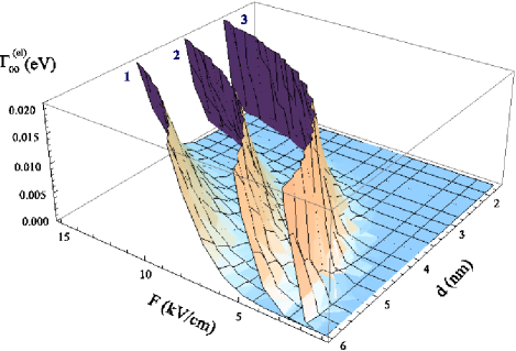
Figure 2: (color online). The width $\Gamma_{00}^{(\mbox{el})}$ (51) of the ground impurity state $n=N=0$ in the GNR placed on the $\mbox{SiO}_{2}$ substrate $(q=0.37)$ as a function of the electric field $F$ and of the graphene width $d$ for the different impurity positions $x_{0}=s\frac{d}{2}$ with $s=0.0-(1),0.5-(2),0.7-(3)$.

The main effect of the electric field is the ionization of the impurity states which are accompanied by the emergence of the energy widths $\Gamma_{Nn}^{(\mbox{el})}$. It follows from eq. (51) that with increasing ribbon width $d$ and strength of the electric fields $F$ the width of the quasi-discrete impurity states increases. However, the greater the shift of the impurity centre $x_{0}$ from the mid-point $x=0$ is the wider the impurity state becomes. This means that in contrast to quasi-1D semiconductor structures (QWR, bulk material subject to a magnetic field) in which the ionization of the impurity centre is reached only by the increasing electric field, in the GNR the mechanism of the dimensional ionization can be realized. The electric field could be kept constant, while the widening of the ribbon and the displacement of the impurity would lead to the ionization. Note, that the dimensional ionization is more efficient as compared to the electric ionization, because the argument of the exponent function in eq. (45) changes $\sim d^{-2}$ with changing the ribbon width $d$, and $\sim F^{-1}$ with changing the electric field $F$. The width $\Gamma_{00}^{(\mbox{el})}$ of the ground impurity state adjacent to the ground size-quantized level $N=0$ as a function of the ribbon width $d$ and electric field $F$ for the different impurity positions $x_{0}$ is depicted in Fig.2. Iso-width lines $F\sim d^{-2}$ providing the width $\Gamma_{00}^{(\mbox{el})}(F,d;x_{0})=\mbox{const.}~{}(x_{0}=\mbox{const.})$ and given in Fig.3 evidently follow from eq. (51).

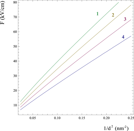
Figure 3: (color online). The iso-width curves $\Gamma_{00}^{(\mbox{el})}(d,F)=\mbox{const.}$ calculated from eq. (51) for the ground impurity state $(n=N=0)$ in the GNR placed on a $\mbox{SiO}_{2}$ substrate $(q=0.37)$. The impurity is positioned at the mid-point $x_{0}=0~{}(s=0)$ of the GNR of width $d$; $F$ is the strength of the electric field. The energy widths are taken to be $\Gamma_{00}^{(\mbox{el})}=0.10-(1),0.060-(2),0.030-(3),0.010-(4)~{}\mbox{eV}$.

Fig.4 demonstrates the iso-width surfaces when all parameters $F,d,x_{0}$ are changed. In the GNRs the effects of both parameters $F$ and $d$ are governed by the exponential factor (45) in contrast to the semiconductor QWR in which the dependence on the radius of the QWR $R$ has the less pronounced logarithmic character monschm09 . Equations (51) and (45) show that the impurity electron becomes practically unbound if the electric field $F$ exceeds the critical value $F^{(\eta)}\simeq F_{0}/\eta^{3}$. Thus, the ground state $(\eta=\delta_{N0})$ is less sensitive to the ionizing effect of the electric field and remains stable up to the significantly greater electric fields $F^{(0)}$ than those $F^{(\eta)}$, destroying the excited states $(\eta\simeq 1,2,\ldots)$.

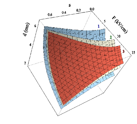
Figure 4: (color online). The iso-width surfaces $\Gamma_{00}^{(\mbox{el})}(d,F,s)=\mbox{const.}$ calculated from eq. (51) for the ground impurity state $(n=N=0)$ in the GNR of width $d$ placed on the $\mbox{SiO}_{2}$ substrate $(q=0.37)$ and exposed to the electric field $F$. The impurity centre is positioned at the coordinate $x_{0}=s\frac{d}{2}$. The energy widths are taken to be $\Gamma_{00}^{(\mbox{el})}=0.010-(1),0.060-(2),0.10-(3)~{}\mbox{in eV}$.

Double subband approximation

The double subband $N=0,1$ approximation describes the combined effect of the electric field ionization and inter-subband autoionization. Since the influence of the electric field was discussed just above here we briefly remind the reader of the sequences of the inter-subband interaction. At $F=0$ the Rydberg series of the strictly discrete energy levels adjacent to the excited size-quantized energies $\varepsilon_{N},~{}(N\neq 0)$ transform into the quasi-discrete levels (Fano resonances) of widths proportional to $\varepsilon_{1}\sim d^{-1}$ and increasing both with decreasing the ribbon width $d$ and with the displacement of the impurity centre from the mid-point of the ribbon $x=0$ monschm12 .

The combined effect of the both types of the ionization reflected in eqs. (62) and (74) leads to the summation of the widths $\Gamma_{Nn}^{(\mbox{el})}$ and $\Gamma_{Nn}^{(\mbox{F})}$, associated with the electric filed and Fano mechanisms, respectively (76). The energy widths $\Gamma_{10}^{(\mbox{el})}$ and $\Gamma_{10}^{(\mbox{F})}$ as a function of the width $d$ for the different strengths $F$ of the electric field and for the impurity positioned at $x_{0}=d/4$ are presented in Fig.5.

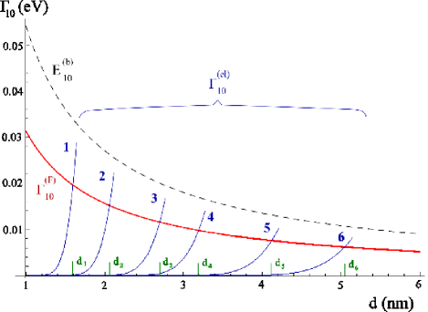
Figure 5: (color online). The dependence of the widths $\Gamma_{10}^{(\mbox{el})}$ (51) and $\Gamma_{10}^{(\mbox{F})}$ (80) of the ground state $n=0$ of the first excited size-quantized Rydberg series $N=1$, caused by the electric field $F$ and the inter-subband coupling, respectively, and the binding energy $E_{10}^{(b)}=\varepsilon_{1}-E_{10}$ on the width $d$ of the GNR placed on the sapphire substrate $q=0.24$. The impurity centre is positioned at the coordinate $x_{0}=0.5\frac{d}{2}$. The electric fields are taken to be $F=2-(1),3-(2),5-(3),7-(4),12-(5),20-(6)~{}\mbox{kV/cm}$. The corresponding critical ribbon widths $d_{F}$ provides the balance between the widths $\Gamma_{10}^{(\mbox{el})}$ and $\Gamma_{10}^{(\mbox{F})}$.

Clearly, $\Gamma_{Nn}^{(\mbox{el})}$ and $\Gamma_{Nn}^{(\mbox{F})}$ change with changing $d$ in the opposite way. As a result in narrow GNRs the widening effect of the Fano coupling exceeds that of the electric field, but with increasing the ribbon width both effects come into balance and then the electric field ionization dominates the autoionization. The greater is the electric field $F$ the less the critical width $d_{F}$ becomes, providing the equality between the both widths. The parameters $d_{F}$ and $F$ obey the relationship $d_{F}^{2}F=\mbox{const.}$, following from the condition $\Gamma_{Nn}^{(\mbox{el})}=\Gamma_{Nn}^{(\mbox{F})}$, in which the widths $\Gamma_{Nn}^{(\mbox{el})}$ and $\Gamma_{Nn}^{(\mbox{F})}$ are given by eqs. (51) and (80), respectively for $N=1,n=0$.

Since the Fano coupling does not contribute to the most interesting ground impurity series $N=0$ and does not manifests itself in not significantly narrow GNRs exposed to sufficiently strong electric fields, we clarify below the mechanism of the resonant capturing of the electron by the impurity centre in the presence of the electric fields. Eqs. (37), (44) show that the ratio $R_{+}/R_{-}=Y/\Gamma(1-\eta)$ for the energy of the ingoing electron $E$ apart from the resonant value $W_{Nn}$ (arbitrary $\eta$ and $Y\sim O(\ln q)$ ) reads $|R_{+}/R_{-}|\gg 1$. The ingoing wave then almost entirely reflects from the barrier. However, under the condition $E\simeq W_{Nn}$ implying $\eta=n+\delta_{Nn}~{},n=0,1,2,\ldots$, eqs. (37), (44) and (46) result in $Y\sim O(\Phi_{Nn}^{2}/\delta_{Nn})$, $|R_{+}/R_{-}|\ll 1$ for the $|R_{-}|^{2}$ given by eq. (81). In case of the exact resonance $(\Delta E=0,w(0)=1)$ the electron density reaches a maximum

$$|R_{-}|^{2}_{\mbox{max}}\sim q^{2}\varepsilon_{N}/\Gamma_{Nn}^{\mbox{(el)}}\gg 1,$$

while for the energy deviations considerably exceeding the resonant width $\Delta E\gg\Gamma_{Nn}^{\mbox{(el)}}$ the electron density reduces relatively $|R_{-}|^{2}_{\mbox{max}}$ by a factor $w(\Delta E)=\left(\Gamma_{Nn}^{\mbox{(el)}}/2\Delta E\right)^{2}\ll 1$. Note, that the probability of the resonant capturing is very sensitive to the accuracy of the resonant energy $W_{Nn}$. Neglecting the deviation of the potential $V_{NN}(y)$ from the Coulomb form $V_{NN}(y)\sim-|y|^{-1}$ (9) at small distances $|y|\ll d$ for which $V_{NN}(y)\sim\ln(|y|/d)$ monschm12 and setting $\delta_{Nn}=0,~{}\eta=n\neq 0$, induce the energy shift $\Delta E=\sim q^{2}\varepsilon_{N}n^{-3}\delta_{Nn}$. This shift significantly exceeding the resonant width $\Gamma_{Nn}^{\mbox{(el)}}$ results in $\Gamma_{Nn}^{\mbox{(el)}}/\Delta E\sim\mbox{O}(\delta_{Nn}^{-1}\Phi_{Nn}^{2})\ll 1$. In conclusion of this paragraph note that the specific problems of the electron scattering on the impurity centres in GNRs having the signs of the resonant and potential scattering require special consideration.

Estimates of the expected experimental values

In an effort to render our results close to an experimental setup, we present below the estimates of the expected values for the GNRs of the family corresponding to $\tilde{\sigma}=\frac{1}{3}$ placed on $\mbox{SiO}_{2}~{}(\epsilon=3.9,q=0.37)$ and sapphire $(\epsilon=10,q=0.24)$ substrates han . Since the $\mbox{SiO}_{2}$ material is not the best candidate to be described by the theory implying $q\ll 1$ the general equation $E^{2}(1+q^{2}/\eta^{2})=\varepsilon_{N}^{2}$ for the energy $E$ has to be taken to calculate the binding energy $E_{N\eta}^{(b)}$, width $\Gamma_{N\eta}$, electric field $F^{(\eta)}$ and other parameters. Being derived from this equation and from eq. $Y(\eta)=0$ (39) the binding energy of the ground Rydberg state $n=0$ of the ground size-quantized series $N=0$ for the impurity positioned at the mid-point $(x_{0}=0)$ of the GNR of width $d=2~{}\mbox{nm}$ reads $E_{00}^{(b)}=68~{}\mbox{meV}$. For the critical electric field $F^{(\eta)}$ providing the complete depletion of the $\eta$ impurity level and estimated from the condition $eF^{(\eta)}a_{0}\eta\simeq E_{N\eta}^{(b)}$ we obtain $F^{(0)}=450~{}\mbox{kV/cm}$. The less bound first excited impurity level $(E_{01}^{(b)}\simeq 54~{}\mbox{meV})$ can be ionized by the electric field $F^{(1)}=310~{}\mbox{kV/cm}$. The above mentioned condition related to the fields $F^{(\eta)}$ is suitable to introduce the parameter of stability $Q_{Nn}(q,s)$ of the $n$ impurity state associated with the $N$ subband relatively to the ionization effect of the electric field $F$

$$Q_{Nn}(q,s) = \frac{\pi^{2}p}{e}|N-\tilde{\sigma}|^{2}G_{Nn}(z);~{}\frac{\pi^{2}p}{e}=6.53~{}\mbox{Vnm};$$ (82)

$$G_{Nn}(z) = 2z\frac{[\sqrt{z^{2}+1}-1]}{z^{2}+1};$$

where $z\equiv z_{Nn}(s)<1$ is the root of the equation $Y(z_{Nn})$ (see eq.(39)). Under the condition $Fd^{2}>Q_{Nn}$ the $Nn$ state is practically ionized, while in the opposite case $Fd^{2}<Q_{Nn}$ the given state can be treated as relatively stable. For the possibly employed substrates, namely $\mbox{SiO}_{2}$ $(q=0.37)$, sapphire $(q=0.24)$ and $\mbox{HfO}_{2}$ $(q=0.13)$ the corresponding parameters calculated for the impurity positioned at the ribbon mid-point $(s=0)$ read $Q_{00}=0.18,~{}0.12,~{}\mbox{and}~{}0.063~{}\mbox{Vnm}$, respectively.

In order to estimate the combined effect of the electric field and Fano-ionization on the impurity states adjacent to the $N=1$ subband we are forced to avoid the ribbon placed on the $\mbox{SiO}_{2}$ substrate and address a sapphire substrate. The point is that the condition of the adiabatic approximation $a_{0}\ll d$ with eq. (11) for $a_{0}$ being written strictly looks like $\pi|N-\tilde{\sigma}|q\ll 1$, which, as pointed above, transforms into eq. (12) for the low excited $N$ subbands. For the chosen $\tilde{\sigma}=1/3$ the ground subband $N=0$ provides for the $\mbox{SiO}_{2}$ substrate $\pi|N-\tilde{\sigma}|q\simeq q\simeq 0.37$, while for the subband $N=1$ this parameter is already $2q=0.74$ that makes the adiabatic approximation for this subband for the $\mbox{SiO}_{2}$ substrate to be inappropriate. It follows from Fig. 5 that the resonant Fano width consists to a considerable part of the binding energy of the ground state $(\Gamma_{10}^{(\mbox{F})}\simeq\frac{2}{3}E_{10}^{(b)})$. The possible reasons for this are first the parameter $q=0.24$ being close to the threshold of the adiabatic approximation $2q\ll 1$ and second the ground state $n=0,\delta_{10}<1$ is more sensitive to the Fano-coupling $\Gamma_{10}^{(\mbox{F})}/E_{10}^{(b)}\sim q\delta_{10}$ than the excited states $n=1,2,\ldots,\Gamma_{n1}^{(\mbox{F})}/E_{1n}^{(b)}\sim q\delta_{1n}^{2}/n,~{}\delta_{1n}<1$. The excited states $n\neq 0$ are expected to be significantly narrower than the ground state $n=0$.

In the presence of relatively weak electric field $F<7~{}\mbox{kV/cm}$ the lifetime $\tau_{10}=\hbar/\Gamma_{10}^{(\mbox{F})}$ of the state $n=0,N=1$ in the ribbon of width $d=2~{}\mbox{nm}$ is determined only by the Fano width $\Gamma_{10}^{(\mbox{F})}\simeq 0.015~{}\mbox{eV}$ resulting in $\tau_{10}=4.4\cdot 10^{-14}~{}\mbox{s}$. However the lifetime of the first excited state $n=N=1$ in the same ribbon $\tau_{11}=\hbar/\Gamma_{11}^{(F)}$ is of the order of $\tau_{11}=1.0\cdot 10^{-12}~{}\mbox{s}$. Thus even in the absence of electric field the resonant Fano widths of the impurity states should be taken into account in the study of the electronic and transport processes in GNRs. Recently Gong et.al. gong reported that the analogous line-defect-induced Fano resonant states in the conduction band of the armchair GNR impede the electron transport in this region. With increasing electric field $F$ and decreasing the ribbon width $d$ the contribution of the electric field to the complete width becomes more pronounced. The critical width $d_{F}$ at which the electric field $F=2,3,5,7,12,20~{}\mbox{kV/cm}$  and the Fano coupling contribute equally to the energy width $\Gamma_{10}^{(\mbox{c})}$ are $d_{F}=5.0,4.1,3.2,2.7,2.0,1.6~{}\mbox{nm}$. The dependence $d_{F}\sim F^{-1/2}$ is valid to a high accuracy. It should be noted that at the critical ribbon widths $d_{F}$ the ground impurity state $n=0$ in the ribbon located on the chosen specific substrate $q=0.24$ seems to be completely ionized. At the same time the substrates with the greater dielectric constant $\epsilon$ (the less $q$) provide significantly stable impurity states especially those having the quantum numbers $n>1$.

A comparison of our results with those obtained numerically based on density functional theory Zhu and on the tight binding approximation Zheng , Jia , Mohamm demonstrates that the Dirac equation approach employed in this paper quite adequately describes the electronic structure and the impurity and exciton states in the GNRs. The exciton characteristics can be obtained from the corresponding impurity ones by replacing $p$ by $2p$ and $q$ by $\frac{1}{2}q$. The dependencies $\sim d^{-1}$ of the effective electron mass $M_{N}=|N-\tilde{\sigma}|\pi\hbar^{2}(pd)^{-1}$ monschm12 , the energy gap $E_{g}=2\varepsilon_{0}$ (5) and the binding energy $E^{(b)}_{\mbox{exc}}=1/2E^{(b)}_{\mbox{imp}}$ (47), (75) on the ribbon width $d$ are qualitatively in line with those presented in all above mentioned Refs. Moreover, the energy gaps $E_{g}$ reveal a quantitative good agreement. Thus, the energy gaps $E_{g}\simeq 0.68~{}\mbox{eV}$ and $E_{g}\simeq 0.89~{}\mbox{eV}$ calculated from (5) for $d=2~{}\mbox{nm}$ and $d=1.45~{}\mbox{nm}$, respectively are close to the values $E_{g}\simeq 0.65~{}\mbox{eV}$ Zheng and $E_{g}\simeq 0.86~{}\mbox{eV}$ Mohamm presented for the corresponding widths. A greater discrepancy is found for the masses $M_{0}\simeq 0.072$ of the electron in the ribbon of width $d\simeq 1.5~{}\mbox{nm}$ scaled to the mass of the free electron $m_{0}$ and $M=0.050$ Mohamm . Though, the dependence $\sim d^{-1}$ of the binding energy on the ribbon width $d$ correlates completely with that obtained numerically Zhu , Jia , Mohamm the different environments prevent us from a detailed quantitative comparison. This is because our data are calculated for the effective dielectric constant $\epsilon_{\mbox{eff}}$ (2) resulting in $q\ll 1$, while others for the GNRs or suspended $(q=2.2)$ Zhu , Jia or placed on the $\mbox{SiO}_{2}$ substrate, with unspecified dielectric constant $\epsilon_{\mbox{eff}}(r)$ (see eqs. (10) and (11) in paper Mohamm ) inducing $q\simeq O(1)$. We therefore conclude that the presented analytical results well correlate with those obtained by the numerical approaches in the literature. Along with the estimates of the expected experimental values this could be extended to further studies of the wide range of the GNR structures and their applications in nanoelectronics.

VI Conclusion

In summary, we have developed an analytical approach to the problem of the impurity electron in a narrow armchair GNR exposed to the external electric field directed parallel to the graphene axis. The effect of the strong confinement is taken to be much greater than the influence of the impurity Coulomb electric field, which in turn considerably exceeds the external field. In the approximation of the isolated size-quantized subbands we have calculated the complex energy levels of the quasi-discrete impurity Rydberg states and phases of the wave functions of the continuous spectrum. The complex energies determine the binding energies and widths of the quasi-stationary states, while the phases (and S-matrix) allow to study the various scattering problems. The explicit form of the obtained results makes it possible to trace the dependence of the listed above values on all the parameters of the structure, namely, on the ribbon width, position of the impurity centre, and the electric field. In particular it was found that the GNR is the structure in which the mechanism of the dimensional ionization occurs: the impurity centre can be ionized by increasing the ribbon width. In the approximation of the ground and first excited size-quantized subbands the complete widths of the first excited Rydberg series caused by the combined effect of the electric fields and the Fano resonant inter-subband coupling have been calculated. Estimates of the expected experimental values for realistic GNGs show that there are two aspects of the effect of the electric field. Weak field provides the resonant capturing of the electrons by the impurity centres for a significantly long lifetime, and remain quasi-discrete impurity states available for the experimental in particular optical study. Relatively strong field releases the bound electrons to activate the transport properties of the GNRs.

VII Acknowledgments

The authors are grateful to D.B. Turchinovich for useful discussions and A. Zampetaki for significant technical assistance.

References

• (1) J. Wang, R. Zhao, M. Yang, Z. Liu, and Z. Liu, J. Chem. Phys. 138 084701 (2013)
• (2) R. B. Biswas, S. Sachdev, and D. T. Son, Phys. Rev. B 76, 205122 (2007)
• (3) D. S. Novikov, Phys. Rev. B 76, 245435 (2007)
• (4) V. M. Pereira, J. Nilsson, and A. H. Castro Neto, Phys. Rev. Lett. 99, 166802 (2007)
• (5) A. V. Shytov, M. I. Katsnelson, and L. S. Levitov, Phys. Rev. Lett. 99, 236801 (2007)
• (6) A. V. Shytov, M. I. Katsnelson, and L. S. Levitov, Phys. Rev. Lett. 99, 246802 (2007)
• (7) T. G. Pedersen, A.-P. Jauho, and K. Pedersen, Phys. Rev. B 79, 113406 (2009)
• (8) K. S. Gupta, S Sen, Phys. Rev. B 78, 205429 (2008)
• (9) B. S. Monozon, P Schmelcher, Phys. Rev. B 86, 245404 (2012)
• (10) A. G. Zhilich and O. A. Maksimov, Sov. Phys. Semicond. 9, 616 (1975)
• (11) B. S. Monozon, and P. Schmelcher, Phys. Rev. B 79, 165314 (2009)
• (12) U. Fano, Phys. Rev. 124, 1866 (1961)
• (13) L. Yang, M. Cohen, S. Louie, Nano Lett. 7, 3112 (2007)
• (14) Y. L. Jia, X. Geng, H. Sun, and Y. Luo, Eur. Phys. J. B 83, 451 (2011)
• (15) L. Mohammadzadeh, A. Asgari, S. Shojaei,E. Ahmadi, Eur. Phys. J. B 84, 249 (2011)
• (16) P. V. Ratnikov and A. P. Silin, JETP 114, 512 (2012)
• (17) V. S. Babichenko, L. V. Keldysh and A. P. Silin, Sov. Phys. Solid. State, 22, 723 (1980)
• (18) L. Brey and H. A. Fertig, Phys. Rev. B 73, 235411 (2006)
• (19) E. H. Hwang and S.Das Sarma, Phys. Rev. B 75, 205418 (2007)
• (20) A. H. Castro Neto, F. Guinea, N. M. R. Peres, K. S. Novoselov, and A. K. Geim, Rev. Mod. Phys. 81 109 (2009)
• (21) Handbook of Mathematical Functions, edited by M. Abramowitz and I. A. Stegun (Dover, New York, 1972)
• (22) F. Sauter, Z. Phys. 69, 742 (1931)
• (23) S. Yu. Slavyanov, Asymptotic Solution to the One-dimensional Schrodinger Equation, (Philadelphia, PA: American Mathematical Society) 1996
• (24) L. D. Landau, and E. M. Lifshitz, Quantum Mechanics: Non-Relativistic Theory (Pergamon, London) 1981
• (25) V. B. Berestetskii, E. M. Lifshitz, L. P. Pitaevskii, Quantum Electrodynamics, Butterworth-Heinemann, Oxford, Second Edition, (1982)
• (26) A. Dalgarno and J. T. Lewis, Proc. Roy Soc. London A 233, 70 (1955)
• (27) P. A. Mello, N. Kumar Quantum Transport in Mesoscopic Systems, (Oxford University Press, New Yor) 1996
• (28) A. I. Baz’, Ya. B. Zel’dovich, and A. M. Perelomov Scattering, Reactions and Decay in Nonrelativistic Quantum Mechanics, (Jerusalem) 1969
• (29) M. Y. Han, J. C. Brant, and P. Kim, Phys. Rev. Lett. 104, 056801 (2010)
• (30) W. J. Gong, X. Y. Sui, L. Zhu, X. Y. Sui, G. D. Yu and X. H. Chen, Europhys. Lett.,103, 18003 (2013)
• (31) X. Zhu and H. Su, J. Phys. Chem. A 115, 11998 (2011)
• (32) H. Zheng, Z. F. Wang, T. Luo, Q. W. Shi, and J. Chen, Phys. Rev. B 75, 165414 (2007)