VoG: Summarizing and Understanding Large Graphs

Abstract

How can we succinctly describe a million-node graph with a few simple sentences? How can we measure the ‘importance’ of a set of discovered subgraphs in a large graph? These are exactly the problems we focus on. Our main ideas are to construct a ‘vocabulary’ of subgraph-types that often occur in real graphs (e.g., stars, cliques, chains), and from a set of subgraphs, find the most succinct description of a graph in terms of this vocabulary. We measure success in a well-founded way by means of the Minimum Description Length (MDL) principle: a subgraph is included in the summary if it decreases the total description length of the graph.

Our contributions are three-fold: (a) formulation: we provide a principled encoding scheme to choose vocabulary subgraphs; (b) algorithm: we develop VoG, an efficient method to minimize the description cost, and (c) applicability: we report experimental results on multi-million-edge real graphs, including Flickr and the Notre Dame web graph.

1 Introduction

Given a large graph, say, a social network like Facebook, what can we say about its structure? As most real graphs, the edge distribution will likely follow a power law [14], but apart from that, is it random? If not, how can we efficiently and in simple terms summarize which parts of the graph stand out, and how? The focus of this paper is exactly finding short summaries for large graphs, in order to gain a better understanding of their characteristics.

Why not apply one of the many community detection, clustering or graph-cut algorithms that abound in the literature [8, 20, 27, 17, 11], and summarize the graph in terms of its communities? The answer is that these algorithms do not quite serve our goal. Typically they detect numerous communities without explicit ordering, so a principled selection procedure of the most “important” subgraphs is still needed. In addition to that, these methods merely return the discovered communities, without characterizing them (e.g., clique, star), and, thus, do not help the user gain further insights in the properties of the graph.

In this paper, we propose VoG, an efficient and effective method to summarize and understand large real-world graphs, in particular graphs beyond the so-called “cavemen” networks that only consist of well-defined, tightly-knit clusters (cliques or near-cliques).

The first insight is to best describe the structures in a graph using an enriched set of “vocabulary” terms: cliques and near-cliques (which are typically considered by community detection methods), and also stars, chains and (near) bi-partite cores. The reasons we have chosen these “vocabulary” terms are: (a) (near-) cliques are included, and so our method works fine on “cavemen” graphs, and (b) stars [16], chains [30] and bi-partite cores [18, 27] appear very often, and have semantic meaning (e.g., factions, bots) in the tens of real networks we have seen in practice (e.g., IMDB movie-actor graph, co-authorship networks, netflix movie recommendations, US Patent dataset, phonecall networks).

The second insight is to formalize our goal as a lossless compression problem, and use the MDL principle. The best summary of a graph is the set of subgraphs that describes the graph most succinctly, i.e., compresses it best, and, thus, helps a human understand the main graph characteristics in a simple, non-redundant manner. A big advantage is that our approach is parameter-free, as at any stage MDL identifies the best choice: the one by which we save most bits.

Informally, we tackle the following problem:

Problem 1 (Informal)

Given: a graph

Find: a set of possibly overlapping subgraphs

to most succinctly describe the given graph, i.e., explain as many of its edges in as simple possible terms,

in a scalable way, ideally linear on the number of edges.

and our contributions can be summarized as:

Problem Formulation: We show how to formalize the intuitive concept of graph understanding using principled, information theoretic arguments.

Effective and Scalable Algorithm: We design VoG which is near-linear on the number of edges.

Experiments on Real Graphs: We empirically evaluate VoG on several real, public graphs spanning up to millions of edges. VoG spots interesting patterns like ‘edit wars’ in the Wikipedia graphs (Fig. 1).

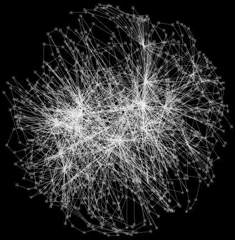
(a) Original Wikipedia Controversy graph (with ‘spring embedded’ layout [15]). No structure stands out.

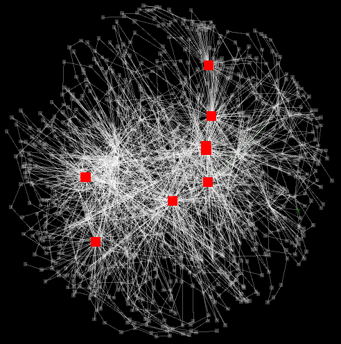
(b) VoG: 8 out of the 10 most informative structures are stars (their centers in red - Wikipedia editors, heavy contributors etc.).

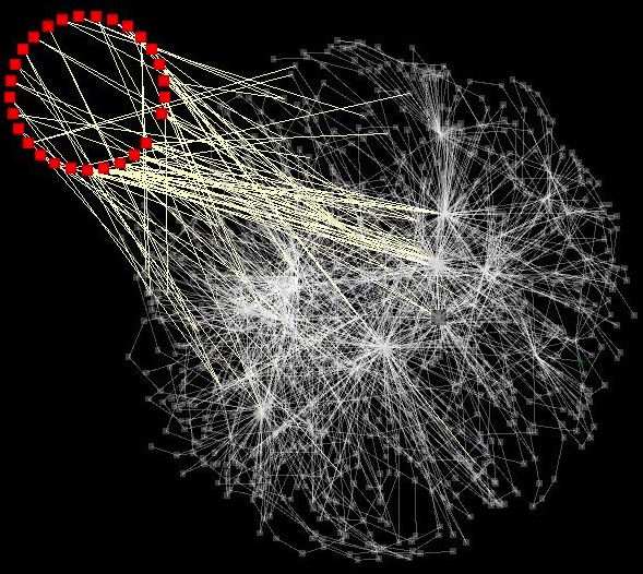
(c) VoG: The most informative bipartite graph - ‘edit war’ - warring factions (one of them, in the top-left red circle), changing each-other’s edits.

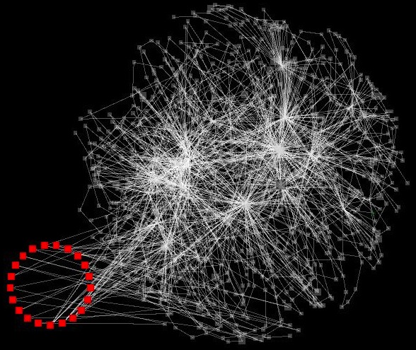
(d) VoG: the second most informative bipartite graph - another ‘edit war’, between vandals (bottom left circle of red points) vs responsible editors (in white).

Figure 1: VoG: summarization and understanding of the most informative, from an information theoretic point of view, structures of the Wikipedia Controversy graph. Nodes stand for Wikipedia contributors and edges link users who edited the same part of the article. Without VoG, in 1(a), no clear structures stand out. VoG spots stars in 1(b) (Wikipedia editors and other heavy contributors), and bipartite graphs in 1(c) and 1(d) (reflecting ‘edit wars’, i.e., editors reverting others’ edits). Specifically, 1(c) shows the dispute between the two parties about a controversial topic and 1(d) shows vandals (red circles) vs responsible Wikipedia editors.

The paper outline is standard: overview, problem formulation, method description, experiments, and conclusions. Due to lack of space, we give more details and experiments in the Appendix.

2 Proposed Method: Overview and Motivation

Before we give our two main contributions in the next sections – the problem formulation, and the search algorithm –, we first provide the high-level outline of VoG, which stands for Vocabulary-based summarization of Graphs:

We use MDL to formulate a quality function: a collection ${M}$ of structures (e.g., a star here, cliques there, etc) is as good as its description length $L(G,M)$. Hence, any subgraph or set of subgraphs has a quality score.

We give an efficient algorithm for characterizing candidate subgraphs. In fact, we allow any subgraph discovery heuristic to be used for this, as we define our framework in general terms and use MDL to identify the structure type of the candidates.

Given a candidate set ${\cal C}$ of promising subgraphs, we show how to mine informative summaries, removing redundancy by minimizing the cost. VoG results in a list $M$ of, possibly overlapping subgraphs, sorted in importance order (compression gain). Together these succinctly describe the main connectivity of the graph.

The motivation behind VoG is that people cannot easily understand cluttered graphs, whereas a handful of simple structures are easily understood, and often meaningful. Next we give an illustrating example of VoG, where the most ‘important’ vocabulary subgraphs that constitute a Wikipedia article’s (graph) summary are semantically interesting.

Illustrating Example: In Fig. 1 we give the results of VoG on the Wikipedia Controversy graph; the nodes are editors, and editors share an edge if they edited the same part of the article. Figure 1(a) shows the graph using the spring-embedded model [15]. No clear pattern emerges, and thus a human would have hard time understanding this graph. Contrast that with the results of VoG. Figs. 1(b)–1(d) depict the same graph, where we highlight the most important structures (i.e., structures that save the most bits) discovered by VoG.

Stars $\rightarrow$ admins (+ vandals): in Fig. 1(b), with red color, we show the centers of the most important “stars”: further inspection shows that these centers typically correspond to administrators who revert vandalisms and make corrections.

Bipartite cores $\rightarrow$ edit wars: Figs. 1(c) and 1(d) give the two most important near-bipartite-cores. Manual inspection shows that these correspond to edit wars: two groups of editors reverting each others’ changes. For clarity, we denote the members of one group by red nodes (left), and hi-light the edges to the other group in pale yellow.

3 Problem Formulation

In this section we describe the first contribution, the MDL formulation of graph summarization. To enhance readability, we list the most frequently used symbols in Table 1.

In general, the Minimum Description Length principle (MDL) [28], is a practical version of Kolmogorov Complexity [21], which embraces the slogan Induction by Compression. Given a set of models $\mathcal{M}$, the best model $M\in\mathcal{M}$ minimizes $L(M)+L(\mathcal{D}\mid M)$, in which $L(M)$ is the length in bits of the description of $M$, and $L(\mathcal{D}\mid M)$ is the length of the description of the data encoded with $M$. To ensure fair comparison, MDL requires descriptions to be losslesss

We consider undirected graphs $G(\mathcal{V},\mathcal{E})$ of $n=|\mathcal{V}|$ nodes, and $m=|\mathcal{E}|$ edges, without self-loops. Our theory, however, can be easily generalized to graphs in general.

Table 1: Description of major symbols.

Notation	Description
$G$	graph
${\mathbf{A}}$	adjacency matrix of $G$
$\mathcal{V}$, $n$	node-set, # of nodes of $G$ respectively
$\mathcal{E}$, $m$	edge-set, # of edges of $G$ respectively
fc, nc	full and near clique respectively
fb, nb	full and near bipartite core respectively
st, ch	star, chain resp.
$\Omega$	vocabulary of structure types
$\mathcal{C},\mathcal{C}_{\mathit{x}}$	set of all/type $x\in\Omega$ candidate structures
${\mathit{M}}$	our model, essentially list of structures
$s,t$	structures in ${\mathit{M}}$
$\mathit{area}(s)$	edges of $G$ (= cells of ${\mathbf{A}}$) described by $s$
$|S|$, $|s|$	cardinality of set $S$, # of nodes of $s$ respectively
$||s||,||s||^{\prime}$	# of existing and non-existing edges in $s$ respectively
${\mathbf{M}}$	approximation of ${\mathbf{A}}$ deduced by $M$
${\mathbf{E}}$	error matrix, ${\mathbf{E}}$ = ${\mathbf{M}}$ $\oplus$ ${\mathbf{A}}$
$\oplus$	exclusive OR
$L(G,M)$	# of bits to describe $M$, and $G$ using $M$
$L(M)$	# of bits to describe model $M$
$L(s)$	# of bits to describe structure $s$

For the graph summary, we use a set of graph structure types $\Omega$ which we call a vocabulary. Although any graph structure can be a part of the vocabulary, we choose the 6 most common structures in real-world graphs ([18, 27, 30]) that are well-known and understood by the graph mining community: full and near cliques ($\mathit{fc},\mathit{nc}$), full and near bi-partite cores ($\mathit{fb},\mathit{nb}$), stars ($\mathit{st}$), and chains ($\mathit{ch}$). Compactly, we have $\Omega=\{\mathit{fc},\mathit{nc},\mathit{fb},\mathit{nb},\mathit{ch},\mathit{st}\}$. We will formally introduce these types after formalizing our goal.

To use MDL for graph summarization, we need to define what our models $\mathcal{M}$ are, how a model $M\in\mathcal{M}$ describes data, and how we encode this in bits. We do this next.

3.1 MDL for Graph Summarization.

As models ${M}$, we consider ordered lists of graph structures, with possible node (but not edge) overlaps. Each structure $s\in M$ identifies a patch of the adjacency matrix $\mathbf{A}$ and describes how it is connected (Fig 2). We refer to this patch, or more formally the edges $(i,j)\in\mathbf{A}$ that structure $s$ describes, as $\mathit{area}(s,M,\mathbf{A})$, where we omit $M$ and $\mathbf{A}$ whenever clear from context.

Let $\mathcal{C}_{x}$ be the set of all possible structures of type $x\in\Omega$, and $\mathcal{C}$ the union of all of those sets, $\mathcal{C}=\cup_{x}{\mathcal{C}_{x}}$. For example, $\mathcal{C}_{\mathit{fc}}$ is the set of all possible full cliques. Our model family $\mathcal{M}$ then consists of all possible permutations of all possible subsets of $\mathcal{C}$ – recall that the models $M$ are ordered lists of graph structures. By MDL, we are after the $M\in\mathcal{M}$ that best balances the complexity of encoding both $\mathbf{A}$ and $M$.

Figure 2: Illustration of our main idea on a toy adjacency matrix: VoG identifies overlapping sets of nodes, that form vocabulary subgraphs (cliques, stars, chains, etc). With overlap, VoG allows for soft clustering of nodes, as in clique A and near-clique B. Stars look like inverted L shapes (e.g., star C). Chains look like lines parallel to the main diagonal (e.g., chain D).

Our general approach for transmitting the adjacency matrix is as follows. First, we transmit the model $M$. Then, given $M$, we can build the approximation $\mathbf{M}$ of the adjacency matrix, as defined by the structures in $M$; we simply iteratively consider each structure $s\in M$, and fill out the connectivity of $\mathit{area}(s)$ in $\mathbf{M}$ accordingly. As $M$ is a summary, it is unlikely that $\mathbf{M}=\mathbf{A}$. Still, in order to fairly compare between models, MDL requires an encoding to be lossless. Hence, besides $M$, we also need to transmit the error matrix $\mathbf{E}$, which encodes the error w.r.t. $\mathbf{A}$. We obtain $\mathbf{E}$ by taking the exclusive OR between $\mathbf{M}$ and $\mathbf{A}$, i.e., $\mathbf{E}=\mathbf{M}\oplus\mathbf{A}$. Once the recipient knows $M$ and $\mathbf{E}$, the full adjacency matrix $\mathbf{A}$ can be reconstructed without loss.

With this in mind, we have as our main score

$$L(G,M)=L(M)+L(\mathbf{E}),$$

where $L(M)$ and $L(\mathbf{E})$ are the numbers of bits that describe the structures, and the error matrix $\mathbf{E}$ respectively. The formal definition of the problem we tackle in this paper is:

Problem 2 (Minimum Graph Description Problem)

Given a graph $G$ with adjacency matrix $A$, and the graph structure vocabulary $\Omega$, by the MDL principle we are after the smallest model $M$ for which the total encoded length

$$L(G,M)=L(M)+L(\mathbf{E})$$

is minimal, where $\mathbf{E}=\mathbf{M}\oplus\mathbf{A}$ is the error matrix, and $\mathbf{M}$ is an approximation of $\mathbf{A}$ deduced by $M$.

Next, we formalize the encoding of the model and the error matrix.

3.2 Encoding the Model.

For the encoded length of a model $M\in\mathcal{M}$, we have

$$L(M) = L_{\mathbb{N}}(|M|+1)+\log\binom{|M|+\Omega|-1}{|\Omega|-1}$$

$$+\sum_{s\in M}{\big{(}-\log\Pr(x(s)\mid M)+L(s)\big{)}}.$$

First, we transmit the total number of structures in $M$ using $L_{\mathbb{N}}$, the MDL optimal encoding for integers $\geq 1$ [28]. Next, by an index over a weak number composition, we optimally encode the number of structures of each type $x\in\Omega$ in model $M$. Then, for each structure $s\in M$, we encode its type $x(s)$ with an optimal prefix code [12], and finally its structure.

To compute the encoded length of a model, we need to define $L(s)$ per structure type:

Cliques. For a full clique, a set of fully-connected nodes, we first encode the number of nodes, and then their ids:

$$L(\mathit{fc})=L_{\mathbb{N}}(|fc|)+\log\binom{n}{|\mathit{fc}|}.$$

As $M$ generalizes the graph, we do not require that $\mathit{fc}$ is a full clique in $G$. If only few edges are missing, it may still be convenient to describe it as such. Every missing edge, however, adds to the cost of transmitting $\mathbf{E}$.

As long as they stand out from the background distribution, less dense or near-cliques can be as interesting as full-cliques. We encode these as follows:

$$L(\mathit{nc}) = L_{\mathbb{N}}(|\mathit{nc}|)+\log\binom{n}{|\mathit{nc}|}$$

$$+\log(|\mathit{area}(nc)|)+||\mathit{nc}||l_{1}+||\mathit{nc}||^{\prime}l_{0}.$$

We transmit the number and ids of nodes as above, and edges by optimal prefix codes. We write $||\mathit{nc}||$ and $||\mathit{nc}||^{\prime}$ for resp. the number of present and missing edges in $\mathit{area}(\mathit{nc})$. Then, $l_{1}=-\log((||\mathit{nc}||/(||\mathit{nc}||+||\mathit{nc}||^{\prime}))$, and analogue for $l_{0}$, are the lengths of the optimal prefix codes for resp. present and missing edges. The intuition is that the more dense/sparse a near-clique is, the cheaper encoding it becomes. Note that this encoding is exact; no edges are added to $\mathbf{E}$.

Bipartite Cores. Bipartite cores are defined as non-empty, non-intersecting sets of nodes, $A$ and $B$, for which there are edges only between the sets $A$ and $B$, and not within.

The encoded length of a full bipartite core $\mathit{fb}$ is

$$L(\mathit{fb})=L_{\mathbb{N}}(|A|)+L_{\mathbb{N}}(|B|)+\log\binom{n}{|A|,|B|},$$

where we encode the size of $A$, $B$, and then the node ids.

As for cliques, for a near bi-partite cores $\mathit{nb}$ we have

$$L(\mathit{nb}) = L_{\mathbb{N}}(|A|)+L_{\mathbb{N}}(|B|)+\log\binom{n}{|A|,|B|}$$

$$+\log(|\mathit{area}(nb)|)+||\mathit{nb}||l_{1}+||\mathit{nb}||^{\prime}l_{0}.$$

Stars. A star is specific case of the bipartite core that consists of a single node (hub) in $A$ connected to a set $B$ of at least 2 nodes (spokes). For $L(\mathit{st})$ of a given star $st$ we have

$$L(\mathit{st})=L_{\mathbb{N}}(|\mathit{st}|-1)+\log n+\log\binom{n-1}{|\mathit{st}|-1},$$

where $|\mathit{st}|-1$ is the number of spokes. We identify the hub out of $n$ nodes, and the spokes from the remainder.

Chains. A chain is a list of nodes such that every node has an edge to the next node, i.e. under the right permutation of nodes, $\mathbf{A}$ has only the super-diagonal elements (directly above the diagonal) non-zero. As such, for the encoded length $L(\mathit{ch})$ for a chain $\mathit{ch}$ we have

$$L(\mathit{ch})=L_{\mathbb{N}}(|\mathit{ch}|-1)+\sum_{i=0}^{|\mathit{ch}|}{\log(n-i)},$$

where we first encode the number of nodes in the chain, and then their ids in order. Note $\sum_{i=0}^{|\mathit{ch}|}{\log(n-i)}\leq|\mathit{ch}|\log n$.

3.3 Encoding the Error.

Next, we discuss how we encode the errors made by $\mathbf{M}$ with regard to $\mathbf{A}$ and store the information in the encoding matrix $\mathbf{E}$. While there are many possible approaches, not all are equally good: we know that the more efficient our encoding is, the less spurious ‘structure’ will be discovered [23].

We hence follow [23] and encode $\mathbf{E}$ in two parts, $\mathbf{E}^{+}$ and $\mathbf{E}^{-}$. The former corresponds to the area of $\mathbf{A}$ that $M$ does model, and for which $\mathbf{M}$ includes superfluous edges. Analogue, $\mathbf{E}^{-}$ consists of the area of $\mathbf{A}$ not modeled by $M$, for which $\mathbf{M}$ lacks edges. We encode these separately as they are likely to have different error distributions. Note that as we know near cliques and near bipartite cores are encoded exactly, we ignore these areas in $\mathbf{E}^{+}$. We encode the edges of $\mathbf{E}^{+}$, and $\mathbf{E}^{-}$ similarly as we do for near-cliques:

$$L(\mathbf{E}^{+}) =\log(|\mathbf{E}^{+}|)+||\mathbf{E}^{+}||l_{1}+||\mathbf{E}^{+}||^{\prime}l_{0}\quad$$

$$L(\mathbf{E}^{-}) =\log(|\mathbf{E}^{-}|)+||\mathbf{E}^{-}||l_{1}+||\mathbf{E}^{-}||^{\prime}l_{0}\quad$$

That is, we first encode the number of $1$s in $\mathbf{E}^{+}$ (or  $\mathbf{E}^{-}$), after which we transmit the $1$s and $0$s using optimal prefix codes. We choose prefix codes over a binomial as this allows us to efficiently calculate local gain estimates in our algorithm without sacrificing much encoding efficiency.

Remark. Clearly, for a graph of $n$ nodes, the search space $\mathcal{M}$ is enormous, as it consists of all possible permutations of the collection $\mathcal{C}$ of all possible structures over the vocabulary $\Omega$. Unfortunately, it does not exhibit trivial structure, such as (weak) (anti)monotonicity, that we could exploit for efficient search. Further, Miettinen and Vreeken [24] showed that for a directed graph finding the MDL optimal model of only full-cliques is NP-hard. Hence, we resort to heuristics.

4 VoG: Summarization Algorithm

Now that we have the arsenal of graph encoding based on the vocabulary of structure types, $\Omega$, we move on to the next two key ingredients: finding good candidate structures, i.e., instantiating $\mathcal{C}$, and then mining informative graph summaries, i.e., finding the best model $M$. The pseudocode of VoG is given in Algorithm 1, and the code is available for research purposes at www.cs.cmu.edu/~dkoutra/SRC/VoG.tar .

4.1 Step 1: Subgraph Generation.

Any combination of clustering and community detection algorithms can be used to decompose the graph into subgraphs. These include, but are not limited to Cross-asssociations [8], Subdue [11], SlashBurn [16], Eigenspokes [27], and METIS [17].

4.2 Step 2: Subgraph Labeling.

Given a subgraph from the set of clusters / communities discovered in the previous step, we search for the structure $x\in\Omega$ that best characterizes it, with no or some errors (e.g., perfect clique, or clique with some missing edges, encoded as error).

Step 2.1: Labeling Perfect Structures. First, the subgraph is tested against our vocabulary structure types for error-free match: full clique, chain, bipartite core, or star. The test for clique or chain is based on its degree distribution. A subgraph is bipartite graph if the magnitudes of its maximum and minimum eigenvalues are equal. To find the node ids in the two node sets, A and B, we use BFS (Breadth First Search) with node coloring. If one of the node sets has size 1, then the given substructure is encoded as star.

Step 2.2: Labeling Approximate Structures. If the subgraph does not belong to $\Omega$, the search continues for the vocabulary structure type that, in MDL terms, best approximates the subgraph. To this end, we encode the subgraph as each of the 6 candidate vocabulary structures, and choose the structure that has the lowest encoding cost.

Let $m^{*}$ be the graph model with only one subgraph encoded as structure $\in\Omega$ (e.g., clique) and the additional edges included in the error matrix. For reasons of efficiency, instead of calculating the full cost $L(G,m^{*})$ as the encoding cost of each subgraph representation, we estimate the local encoding cost $L(m^{*})+L(\mathbf{E}^{+}_{m^{*}})+L(\mathbf{E}^{-}_{m^{*}})$, where $\mathbf{E}^{+}_{m^{*}}$ and $\mathbf{E}^{-}_{m^{*}}$ encode the incorrectly modeled, and unmodeled edges respectively (Sec. 3). The challenge of the step is to efficiently identify the role of each node in the subgraph (e.g., hub/spoke in a star, member of set $A$ or $B$ in a near-bipartite core, order of nodes in chain) for the MDL representation. We elaborate on each structure next.

Clique. This is the simplest representation, as all the nodes have the same structural role. For near-cliques we ignore $\mathbf{E_{\mathit{nc}}}$, and, so, the encoding cost is $L(\mathit{nc})$.

Star. The highest-degree node of the subgraph is encoded as the hub, and the rest nodes as spokes.

Bipartite core. In this case, the problem of identifying the role of each node reduces to finding the maximum bipartite graph, which is known as max-cut problem, and is NP-hard. The need of a scalable graph summarization algorithm makes us resort to approximation algorithms. Finding the maximum bipartite graph can be reduced to semi-supervised classification. We consider two classes which correspond to the two node sets, $A$ and $B$, of the bipartite graph, and the prior knowledge is that the highest-degree node belongs to $A$, and its neighbors to $B$. To propagate these classes/labels, we employ Fast Belief Propagation (FaBP) [19] assuming heterophily (i.e., connected nodes belong to different classes). For near-bipartite cores $L(\mathbf{E}^{+}_{\mathit{nb}})$ is omitted.

Chain. Representing the subgraph as a chain reduces to finding the longest path in it, which is also NP-hard. Therefore, we employ the following heuristic. Initially, we pick a node of the subgraph at random, and find its furthest node using BFS (temporary start). Starting from the latter and by using BFS again, we find the subsequent furthest node (temporary end). Then we extend the chain by local search. Specifically, we consider the subgraph from which all the nodes that already belong to the chain, except for its endpoints, are removed. Then, starting from the endpoints we employ again BFS. If new nodes are found during this step, they are added in the chain (rendering it a near-chain with few loops). The nodes of the subgraph that are not members of this chain are encoded as error in $\mathbf{E_{\mathit{ch}}}$.

After representing the subgraph as each of the vocabulary structures $x$, we employ MDL to choose the representation with the minimum (local) encoding cost, and add the structure to the candidate set, $\mathcal{C}$. Finally, we associate the candidate structure with its encoding benefit: the savings in bits for encoding the subgraph by the minimum-cost structure type, instead of leaving its edges unmodeled and including them in the error matrix.

Algorithm 1 VoG

  Input: graph $G$

  Step 1: Subgraph Generation. Generate candidate – possibly overlapping – subgraphs using one or more graph decomposition methods.

  Step 2: Subgraph Labeling. Characterize each subgraph as a perfect structure $x\in\Omega$, or an approximate structure by using MDL to find the type $x$ that locally minimizes the encoding cost. Populate the candidate set $\mathcal{C}$.

  Step 3: Summary Assembly. Use the heuristics Plain, Top10, Top100, Greedy’nForget (Sec. 4.3) to select a non-redundant subset from the candidate structures to instantiate the graph model ${M}$. Pick the model of the heuristic with the lowest description cost.

  return  graph summary ${M}$ and its encoding cost.

4.3 Step 3: Summary Assembly.

Given a set of candidate structures, $\mathcal{C}$, how can we efficiently induce the model $M$ that is the best graph summary? The exact selection algorithm, which considers all the possible ordered combinations of the candidate structures and chooses the one that minimizes cost, is combinatorial, and cannot be applied to any non-trivial candidate set. Thus, we need heuristics that will give a fast, approximate solution to the description problem. To reduce the search space of all possible permutations, we attach to each candidate structure a quality measure, and consider them in order of decreasing quality. The measure that we use is the encoding benefit of the subgraph, i.e., the number of bits that are gained by encoding the subgraph as structure $x$ instead of noise. Our constituent heuristics are:

  Plain: The baseline approach gives as graph summary all the candidate structures, i.e., $M=\mathcal{C}$.

  Top-k: Selects the top $k$ candidate structures, which are sorted in decreasing quality.

  Greedy’nForget: Considers each structure in $\mathcal{C}$ sequentially, and includes it in $M$: if the graph’s encoding cost does not increase, then it keeps the structure in $M$; otherwise it removes it. Note that this heuristic is computationally demanding, and works better for small and medium-sized set of candidate structures.

VoG employs all the heuristics and picks the best graph summarization, i.e., with the minimum description cost.

5 Experiments

Table 2: [Lower is better.] Quantitative analysis of VoG with different heuristics: Plain, Top10, Top100, and Greedy’nForget. The first column, Original, presents the cost, in bits, of encoding the adjacency matrix with an empty model $M$. For different heuristics we show the relative number of bits needed to describe the adjacency matrix. In parentheses, precursored by ‘u.e.’ (for unexplained edges) we give the fraction of edges that are not explained by the structures in the model, $M$. The lowest description cost is in bold.

Graph		Original		VoG
		(bits)		Plain	Top10	Top100	Greedy’nForget
Flickr		35 210 972		81% (u.e.: 4%)	99% (u.e.: 72%)	97% (u.e.: 39%)	95% (u.e.: 36%)
WWW-Barabasi		18 546 330		81% (u.e.: 3%)	98% (u.e.: 62%)	96% (u.e.: 51%)	85% (u.e.: 38%)
Epinions		5 775 964		82% (u.e.: 6%)	98% (u.e.: 65%)	95% (u.e.: 46%)	81% (u.e.: 14%)
Enron		4 292 729		75% (u.e.: 2%)	98% (u.e.: 77%)	93% (u.e.: 46%)	75% (u.e.: 6%)
AS-Oregon		475 912		72% (u.e.: 4%)	87% (u.e.: 59%)	79% (u.e.: 25%)	71% (u.e.: 12%)
Chocolate		60 310		96% (u.e.: 4%)	96% (u.e.: 70%)	93% (u.e.: 35%)	88% (u.e.: 27%)
Controversy		19 833		98% (u.e.: 5%)	94% (u.e.: 51%)	96% (u.e.: 12%)	87% (u.e.: 31%)

In this section, we aim to answer the following questions: Q1.  Are the real graphs structured, or random and noisy?
Q2. What structures do the graph summaries consist of, and how can they be used for understanding?
Q3.  Is VoG scalable?

Table 3: Summary of graphs used.

Name	Nodes		Edges	Description
Flickr [3]	404 733		2 110 078	Friendship social network
WWW-Barabasi [4]	325 729		1 090 108	WWW in nd.edu
Epinions [4]	75 888		405 740	Trust graph
Enron [2]	80 163		288 364	Enron email
AS-Oregon [1]	13 579		37 448	Router connections
Controversy	1 005		2 123	Co-edit graph
Chocolate	2 899		5 467	Co-edit graph

The graphs we use in the experiments along with their descriptions are summarized in Table 3. Controversy is a co-editor graph on a known Wikipedia controversial topic (name withheld for obvious reasons), where the nodes are users and edges mean that they edited the same sentence. Chocolate is a co-editor graph on the ‘Chocolate’ article. The descriptions of the other datasets are given in Table 3.

Graph Decomposition. In our experiments, we use SlashBurn [16] to generate candidate subgraphs, because it is scalable, and designed to handle graphs without “cavemen” structure. Details about the algorithm are given in the Appendix. We note that VoG would only benefit from using the outputs of additional decomposition algorithms.

5.1 Q1: Quantitative Analysis

In this section we apply VoG to the real datasets of Table 3, and evaluate the achieved description cost, and edge coverage, which are indicators of the discovered structures. The evaluation is done in terms of savings w.r.t. the base encoding (Original) of the adjacency matrix of a graph with an empty model $M$.

Although we refer to the description cost of the summarization techniques, we note that compression itself is not our goal, but our means for identifying structures important for graph understanding or attention routing. This is also why we do not compare against standard matrix compression techniques. Whereas VoG has the goal of describing a graph with intelligible structures, specialized algorithms may exploit any statistical correlations to save bits.

We compare two summarization approaches: (a) Original: The whole adjacency matrix is encoded as if it contains no structure; that is, $M=\emptyset$, all of $\mathbf{A}$ is encoded through $L(\mathbf{E}^{-})$; and (b) VoG, our proposed summarization algorithm with the three selection heuristics (Plain, Top10 and Top100, Greedy’nForget). For efficiency, for Flickr and WWW-Barabasi, Greedy’nForget considers the top 500 candidate structures. We note that we ignore very small structures; the candidate set $\mathcal{C}$ includes subgraphs with at least 10 nodes, except for the Wikipedia graphs where the size threshold is set to 3 nodes. Among the summaries obtained by the different heuristics, we choose the one that yields the smallest description length.

Table 2 presents the summarization cost of each technique w.r.t. the cost of the Original approach, as well as the fraction of the edges that remains unexplained. The lower the ratios (i.e., the lower the obtained description length), the more structure is identified. For example, VoG-Plain describes Flickr with only 81% of the bits of the Original approach, and explains all but 4% of the edges, which means that 4% of the edges are not encoded by the structures in $M$.

Observation 1

Real graphs do have structure; VoG, with or w/o structure selection, achieves better compression than the Original approach that assumes no structure.

Greedy’nForget finds models $M$ with fewer structures than Plain and Top100, yet generally obtains (much) succinct graph descriptions. This is due to its ability to identify structures that are informative with regard to what it already knows. In other words, structures that highly overlap with ones already selected into $M$ will be much less rewarded than structures that explain unexplored parts of the graph.

5.2 Q2: Qualitative Analysis

In this section, we showcase how to use VoG and interpret its output.

5.2.1 Graph Summaries

Table 4: Summarization of graphs by VoG (for different heuristics). The most frequent structures are the stars (st) and near-bipartite cores (nb). For each graph and selection technique (heuristic), we provide the frequency of each structure type: ‘st’ for star, ‘nb’ for near-bipartite cores, ‘fc’ for full cliques, ‘fb’ for full bipartite-cores, ‘ch’ for chains, and ‘nc’ for near-cliques.

		Plain							Top10			Top100					Greedy’nForget
Graph		st	nb	fc	fb	ch	nc		st	nb		st	nb	fb	ch		st	nb	fc	fb
Flickr		24 385	3 750	281	9	-	3		10	-		99	1	-	-		415	-	-	1
WWW-Barabasi		10 027	1 684	487	120	26	-		9	1		83	14	3	-		403	7	-	16
Epinions		5 204	528	13	-	-	-		9	1		99	1	-	-		2 738	-	8	-
Enron		3 171	178	3	11	-	-		9	1		99	1	-	-		2 323	3	3	2
AS-Oregon		489	85	-	4	-	-		10	-		93	6	1	-		399	-	-	-
Chocolate		170	58	-	-	17	-		9	1		87	10	-	3		101	-	-	-
Controversy		73	21	-	1	22	-		8	2		66	17	1	16		35	-	-	-

How does VoG summarize real graphs? Which are the most frequent structures? Table 4 shows the summarization results of VoG for different structure selection techniques.

Observation 2

The summaries of all the selection heuristics consist mainly of stars, followed by near-bipartite cores. In some graphs, like Flickr and WWW-Barabasi, there is a significant number of full cliques.

From Table 4 we also observe that Greedy’nForget drops uninteresting structures, and reduces the graph summary. Effectively, it filters out the structures that explain edges already explained by structures in model $M$.

5.2.2 Graph Understanding

Are the ‘important’ structures found by VoG semantically meaningful? For sense-making, we analyze the discovered subgraphs in the non-anonymized real datasets Controversy, and Enron.

Wikipedia–Controversy.

Figs. 1 and 3(a-b) illustrate the original and VoG-based visualization of the Controversy graph. The VoG-Top10 summary consists of 8 stars and 2 near-bipartite cores (see also Table 4). The 8 star configurations correspond mainly to administrators, such as “Future_Perfect_at_sunrise”, who do many minor edits and revert vandalisms. The most interesting structures VoG identifies are the near-bipartite cores, which reflect: (a) the conflict between the two parties, and (b) an “edit war” between vandals and administrators or loyal Wikipedia users.

(a) VoG: The 8 top “important” stars whose centers are denoted with red rectangles.

(b) VoG: The most “important” bipartite graph (node set $A$ denoted by the circle of red points).

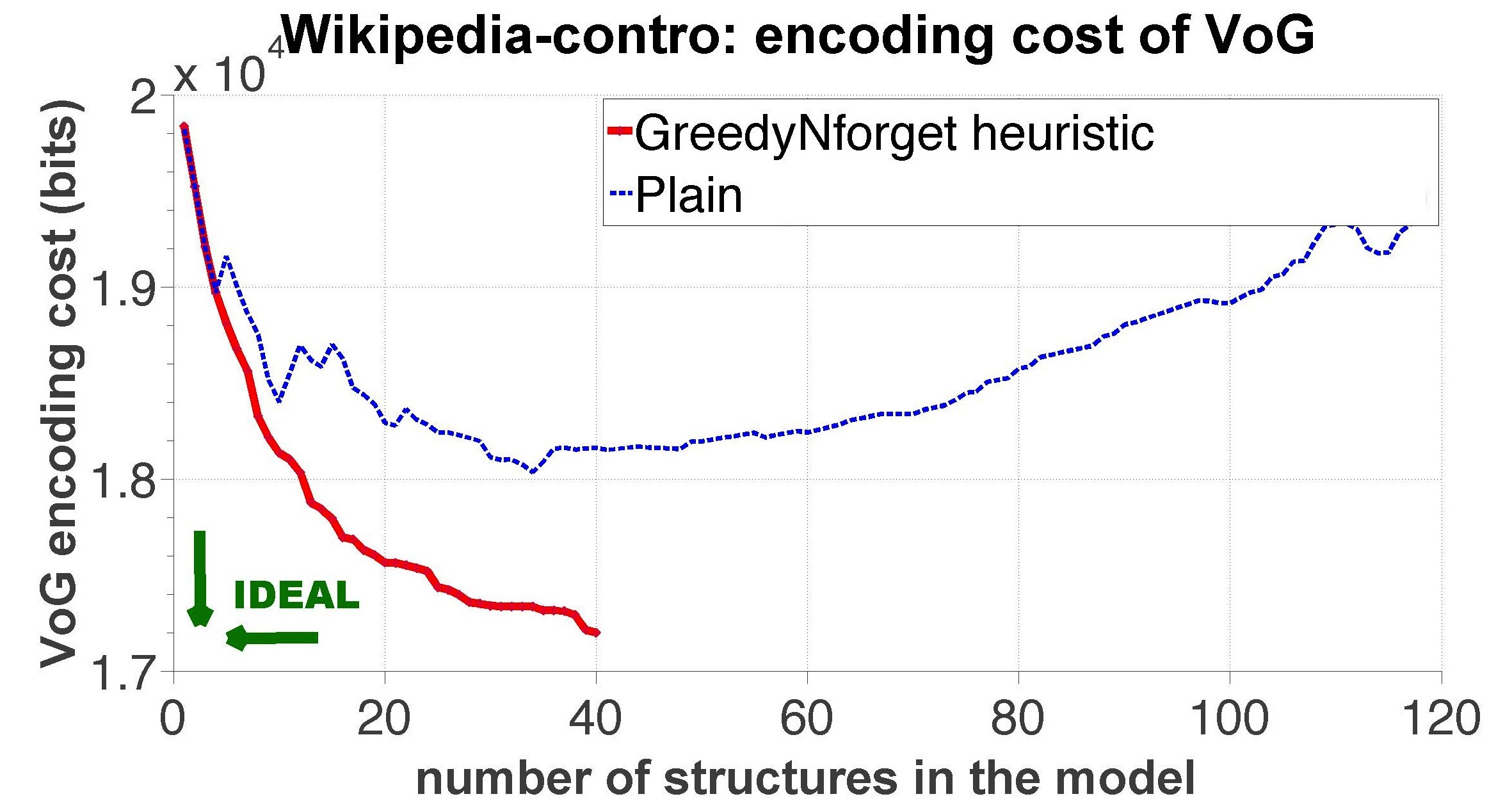
(c) Effectiveness of Greedy’nForget (in red). Encoding cost of VoG vs. number of structures in the model, $M$.

Figure 3: The VoG summary of the Controversy graph, and effectiveness of the Greedy’nForget heuristic. The top 10 structures of the graph summary of VoG consist of 8 stars (Fig. 3(a)) and 2 bipartite graphs (Fig. 3(b), 1(d)). Fig. 3(c) shows the encoding cost for the Plain (dotted blue line) and Greedy’nForget (solid red line) heuristics. Greedy’nForget minimizes the encoding cost by greedily selecting from a sorted, in decreasing quality order, set of structures the ones that reduce the cost. Thus, Greedy’nForget leads to better encoding costs and smaller summaries (here only 40 are chosen) than Plain ($\sim$120 structures).

In Fig. 3(c), the encoding cost of VoG is given as a function of the selected structures. The dotted blue line corresponds to the cost of the Plain encoding, where the structures are added sequentially in the model $M$, in decreasing order of quality (local encoding benefit). The solid red line maps to the cost of the Greedy’nForget heuristic. Given that the goal is to summarize the graph in the most succinct way, and at the same time achieve low encoding cost, Greedy’nForget is effective.

Enron.

The Top10 summary for Enron has nine stars and one near-bipartite core. The centers of the most informative stars are mainly high ranking officials (e.g., Kenneth Lay with two email accounts, Jeff Skilling, Tracey Kozadinos). As a note, Kenneth Lay was long-time Enron CEO, while Jeff Skilling had several high-ranking positions in the company, including CEO and managing director of Enron Capital & Trade Resources. The near-bipartite core in Fig. 4 is loosely connected to the rest of the graph, and represents the email communication about an extramarital affair, which was broadcast to 235 recipients.

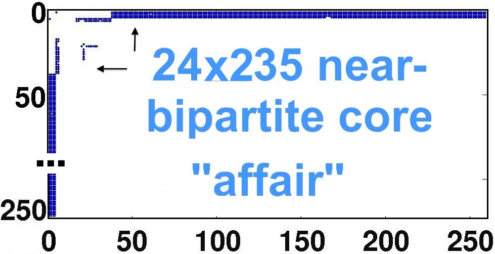
Figure 4: Enron: Adjacency matrix of the top nb core found by VoG, corresponding to email communication about an “affair”.

The VoG summary for Chocolate is equally interesting, but not shown here do to lack of space (see the Appendix).

5.3 Q3: Scalability of VoG

In Fig. 5, we present the runtime of VoG with respect to the number of edges in the input graph. For this purpose, we induce subgraphs of Notre Dame dataset (WWW-Barabasi) for which we give the dimensions in Table 5. We ran the experiments on a Intel(R) Xeon(R) CPU 5160 at 3.00GHz, with 16GB memory. The structure identification is implemented in Matlab, while the selection process in Python. A discussion about the runtime of VoG is also given in the supplementary material.

Observation 3

All the steps of VoG are designed to be scalable. Fig. 5 shows the complexity is $O(m)$, i.e., VoG is near-linear on the number of edges of the input graph.

Table 5: Scalability: Induced subgraphs of WWW-Barabasi.

Name	Nodes	Edges
WWW-Barabasi-50k	49 780	50 624
WWW-Barabasi-100k	99 854	205 432
WWW-Barabasi-200k	200 155	810 950
WWW-Barabasi-300k	325 729	1 090 108

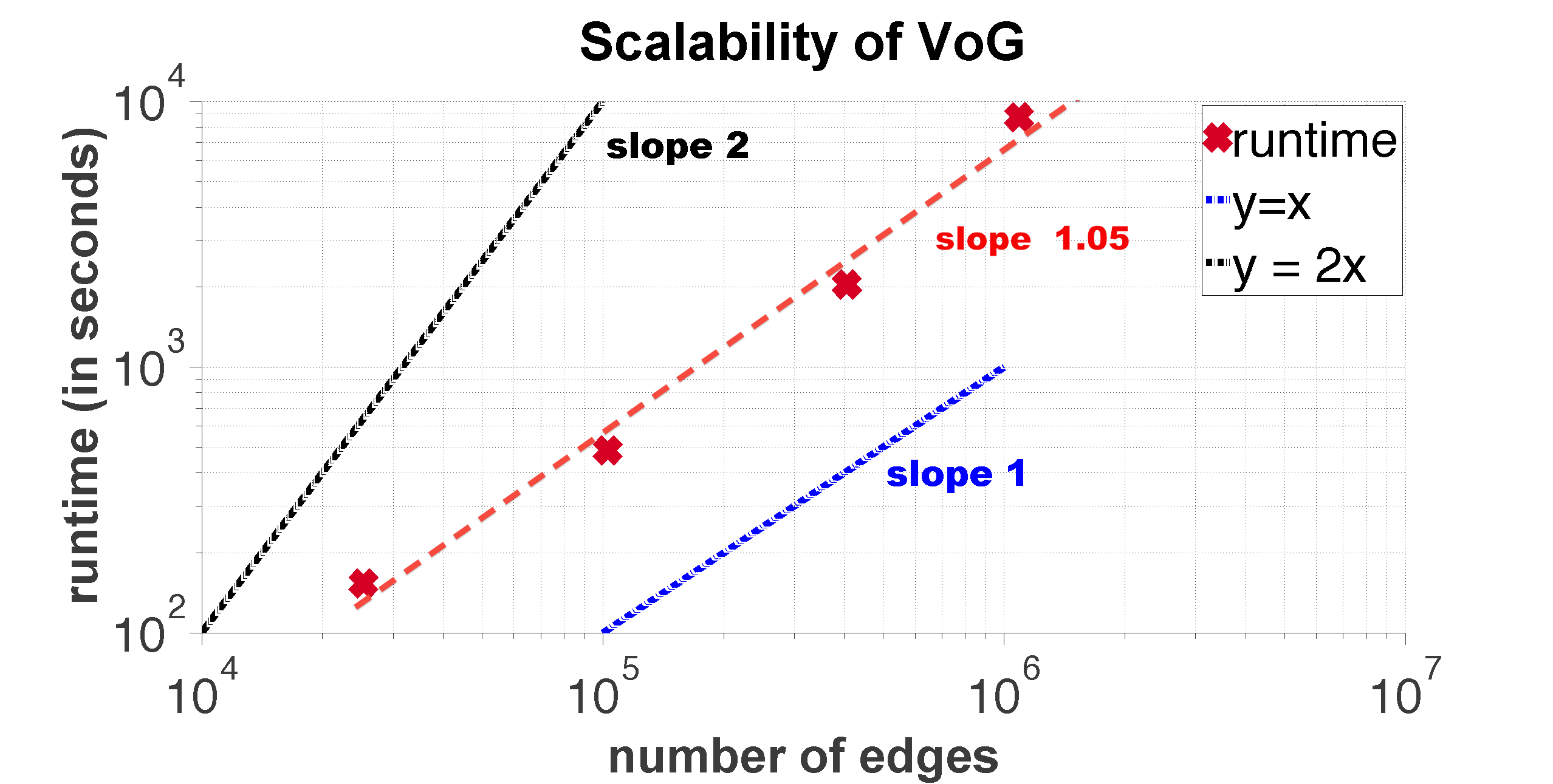
Figure 5: VoG is near-linear on the number of edges. Runtime, in seconds, of VoG (Plain) vs.  number of edges in graph. For reference we show the linear and quadratic slopes.

6 Discussion

The experiments show that VoG successfully solves an important open problem in graph understanding: how to find a succinct summary for a large graph. Here we address some questions, that a reader may have.

Q1: Why does VoG use the chosen vocabulary structures (stars, cliques, etc), and not other structures?

A1: We noticed that these structures appear very often, in tens of real graphs, (e.g. in patent citation network, in phone-call networks, in netflix recommendation system, etc).

Q2: What if a new structure (say, ‘loops’), proves to be frequent in real graphs?

A2: VoG can easily be extended to handle new vocabulary terms. In fact, MDL will immediately tell us whether a vocabulary set ${\cal V}_{1}$ is better than a vocabulary set ${\cal V}_{2}$: the one that gives best compression wins!

Q3: Why not determine automatically which ‘vocabulary terms’ are best for a given graph?

A3: Scalability. Spotting frequent subgraphs has the notoriously-expensive subgraph isomorphism problem in the inner loop. Published algorithms on frequent subgraphs (e.g., [34]), are not applicable here, since they expect the nodes to have labels (e.g., carbon atom, oxygen atom etc.).

Q4: Why would you focus on compression, since your goal is pattern discovery and understanding?

A4: Compression is not our goal; it is only our means to help us find good patterns. High compression ratios are exactly a sign that we discovered many redundancies (i.e., patterns) which can be explained in simple terms (i.e., structures), and thus, we understand the input graph better.

7 Related Work

Work related to VoG comprises the following areas:

MDL for Non-Graph Data. The MDL principle [28] and compression  [13] are related to summarization and pattern discovery ( e.g., clustering [10], pattern set mining [33]).

Graph Compression. This includes lexicographic-based compression for web [6], and social networks  [9]; BFS-based techniques [5]; multi-position linearizations for neighborhood queries [22]; exploitation of the power-laws in real graphs  [20] and structural equivalence [32]; attribute-based, non-overlapping and covering node grouping [31, 35]. None of these works summarize in terms of local structures. Also, compression is not our goal, but our means to understanding the graph, by finding informative structures.

Graph Partitioning. Assuming away the ‘no good cut’ issue, there are countless graph partitioning algorithms: Subdue [11], a frequent subgraph mining algorithm for lossy summaries of attributed graphs; iterative, non-overlapping grouping of nodes with high inter-connectivity [25]; MDL-based Boolean matrix factorization for mining full cliques [23]; cross-association for near cliques and bi-partite cores. [7], or hierarchies [26]; information-theoretic approaches for community detection [29].

What sets VoG apart: None of the above methods meet all the following specifications (which VoG does): (a) gives a soft clustering, (b) is scalable, (c) has a large vocabulary of graph primitives (beyond cliques/cavemen-graphs) and (d) is parameter-free.

8 Conclusion

We studied the problem of succinctly describing a large graph in terms of connectivity structures. Our contributions are:

• Problem Formulation: We proposed an information theoretic graph summarization technique that uses a carefully chosen vocabulary of graph primitives (Sec. 3).

• Effective and Scalable Algorithm: We gave VoG, an effective method which is near-linear on the number of edges of the input graph (Sec. 5.3).

• Experiments on Real Graphs: We discussed interesting findings like exchanges between Wikipedia vandals and responsible editors on large graphs (Sec. 1, 5).

A SlashBurn: Details

SlashBurn is an algorithm for node reordering so that the resulting adjacency matrix has clusters/patches of non-zero elements. The idea is that removing the top high-degree nodes in real world graphs results in the generation of many small-sized disconnected components (subgraphs), and one giant connected component whose size is significantly smaller compared to the original graph. Specifically, SlashBurn performs two steps iteratively: (a) It removes top high degree nodes from the original graph; (b) It reorders the nodes so that the high-degree nodes go to the front, disconnected components to back, and the giant connected component to the middle. During the next iterations, these steps are performed on the giant connected component.

In this paper, SlashBurn is used to decompose graphs, and MDL is used to select an appropriate model to encode the subgraphs.

B Toy Example

To illustrate how VoG works, we give an example on a toy graph; we apply VoG on the synthetic Cavemen graph of 841 nodes and 7547 edges, which as shown in Fig. 6 consists of two cliques separated by two stars. The leftmost and rightmost cliques consist of 42, and 110 nodes respectively; the big star (2nd structure) has 800 nodes, and the small star (3rd structure) 91 nodes.

The raw output of the decomposition algorithm (step 1) consists of the subgraphs corresponding to the stars, the full left-hand and right-hand cliques, as well as subsets of these nodes. Through MDL, VoG first correctly identifies the type of these structures (step 2), and through Greedy’nForget it automatically finds the true 4 structures without redundancy (step 3). The corresponding model requires 36% fewer bits than the ‘empty’ model. We note that one bit gain already corresponds to twice the likelihood.

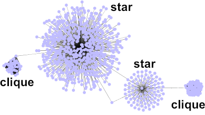
Figure 6: Toy graph for sanity check: VoG saves 36% in space, by successfully discovering the two cliques and two stars that we chained together.

C Time Complexity of VoG

For a graph $G(\mathcal{V},\mathcal{E})$ of $n=|\mathcal{V}|$ nodes and $m=|\mathcal{E}|$ edges, the time complexity of VoG depends on the runtime complexity of the algorithms that compose it, namely the decomposition algorithm, the subgraph labeling, the encoding scheme $L(G,M)$ of the model, and the structure selection (summary assembly).

For the decomposition of the graph, we use SlashBurn which is near-linear on the number of edges of real graphs [16]. The subgraph labeling algorithms in Sec. 4 are carefully designed to be linear in the number of edges of the input subgraph.

When there is no overlap between the structures in $M$, the complexity of calculating the encoding scheme $L(G,M)$ is $O(m)$. When there is overlap, the complexity is bigger: assume that $s,t$ are two structures $\in M$ with overlap, and $t$ has higher quality than $s$, i.e., $t$ comes before $s$ in the ordered list of structures. Finding how much ‘new’ structure (or area in ${\mathbf{A}}$) $s$ explains relative to $t$ costs $O(|M|^{2})$. Thus, in the case of overlapping subgraphs, the complexity of computing the encoding scheme is $O(|M|^{2}+m)$. As typically $|M|\ll m$, in practice we have $O(m)$.

As far as the selection method is concerned, the Top-k heuristic that we propose has complexity $O(k)$. The Greedy’nForget heuristic has runtime $O(|\mathcal{C}|\times o\times m)$, where $|\mathcal{C}|$ is the number of structures identified by VoG, and $o$ the time complexity of $L(G,M)$.

D Qualitative Analysis of VoG

In addition to the analysis of Controversy and Enron in Sec. 5.2.1, we present qualitative results on the Chocolate dataset.

Wikipedia–Chocolate.

The visualization of Wikipedia-choc is similar to Fig. 3 and is omitted. As shown in Table 4, the Top10 summary of Chocolate contains 9 stars and 1 near-bipartite core. The center of the highest ranked star corresponds to “Chobot”, a Wikipedia bot that fixes interlanguage links, and thus touches several, possibly unrelated parts of a page. Other stars have as hubs administrators, who do many minor edits, as well as heavy contributors. The near-bipartite core captures the interactions between possible vandals and administrators (or Wikipedia contributors) who were reverting each other’s edits resulting to temporary (semi-) protection of the webpage.

References

- [1] As-oregon dataset. http://topology.eecs.umich.edu/data.html.
- [2] Enron dataset. http://www.cs.cmu.edu/ enron.
- [3] Flickr. http://www.flickr.com.
- [4] Snap. http://snap.stanford.edu/data/index.html.
- [5] A. Apostolico and G. Drovandi. Graph compression by bfs. Algorithms, 2(3):1031–1044, 2009.
- [6] P. Boldi and S. Vigna. The webgraph framework i: compression techniques. In WWW, 2004.
- [7] D. Chakrabarti, S. Papadimitriou, D. S. Modha, and C. Faloutsos. Fully automatic cross-associations. In KDD, pages 79–88, 2004.
- [8] D. Chakrabarti, Y. Zhan, D. Blandford, C. Faloutsos, and G. Blelloch. Netmine: New mining tools for large graphs. In SDM Workshop on Link Anal., Count. Terror. and Priv., 2004.
- [9] F. Chierichetti, R. Kumar, S. Lattanzi, M. Mitzenmacher, A. Panconesi, and P. Raghavan. On compressing social networks. In KDD, pages 219–228, 2009.
- [10] R. Cilibrasi and P. Vitányi. Clustering by compression. IEEE TIT, 51(4):1523–1545, 2005.
- [11] D. J. Cook and L. B. Holder. Substructure discovery using minimum description length and background knowledge. JAIR, 1:231–255, 1994.
- [12] T. M. Cover and J. A. Thomas. Elements of Information Theory. Wiley-Interscience New York, 2006.
- [13] C. Faloutsos and V. Megalooikonomou. On data mining, compression and Kolmogorov complexity. In Data Min. Knowl. Disc., volume 15, pages 3–20. Springer-Verlag, 2007.
- [14] M. Faloutsos, P. Faloutsos, and C. Faloutsos. On power-law relationships of the internet topology. In SIGCOMM, pages 251–262, 1999.
- [15] T. Kamada and S. Kawai. An algorithm for drawing general undirected graphs. IPL, 31:7–15, 1989.
- [16] U. Kang and C. Faloutsos. Beyond ‘caveman communities’: Hubs and spokes for graph compression and mining. In ICDM, 2011.
- [17] G. Karypis and V. Kumar. Multilevel -way hypergraph partitioning. In DAC, pages 343–348, 1999.
- [18] J. Kleinberg, R. Kumar, P. Raghavan, S. Rajagopalan, and A. Tomkins. The web as a graph: Measurements, models and methods. In COCOON, 1999.
- [19] D. Koutra, T.-Y. Ke, U. Kang, D. H. Chau, H.-K. K. Pao, and C. Faloutsos. Unifying guilt-by-association approaches: Theorems and fast algorithms. In ECML PKDD, pages 245–260, 2011.
- [20] J. Leskovec, K. J. Lang, A. Dasgupta, and M. W. Mahoney. Statistical properties of community structure in large social and information networks. In WWW, pages 695–704, 2008.
- [21] M. Li and P. Vitányi. An Introduction to Kolmogorov Complexity and its Applications. Springer, 1993.
- [22] H. Maserrat and J. Pei. Neighbor query friendly compression of social networks. In KDD, 2010.
- [23] P. Miettinen and J. Vreeken. Model order selection for Boolean matrix factorization. In KDD, pages 51–59, 2011.
- [24] P. Miettinen and J. Vreeken. mdl4bmf: Minimum Description Length for Boolean matrix factorization. Technical Report MPI-I-2012-5-001, MPI-Inf, 2012.
- [25] S. Navlakha, R. Rastogi, and N. Shrivastava. Graph summarization with bounded error. In SIGMOD, pages 419–432, 2008.
- [26] S. Papadimitriou, J. Sun, C. Faloutsos, and P. S. Yu. Hierarchical, parameter-free community discovery. In ECML PKDD, 2008.
- [27] B. A. Prakash, M. Seshadri, A. Sridharan, S. Machiraju, and C. Faloutsos. Eigenspokes: Surprising patterns and community structure in large graphs. PAKDD, 2010.
- [28] J. Rissanen. Modeling by shortest data description. Annals Stat., 11(2):416–431, 1983.
- [29] M. Rosvall and C. T. Bergstrom. An information-theoretic framework for resolving community structure in complex networks. PNAS, 104(18):7327–7331, 2007.
- [30] L. Tauro, C. Palmer, G. Siganos, and M. Faloutsos. A simple conceptual model for the internet topology. Globecom, 2001.
- [31] Y. Tian, R. A. Hankins, and J. M. Patel. Efficient aggregation for graph summarization. In SIGMOD, pages 567–580, 2008.
- [32] H. Toivonen, F. Zhou, A. Hartikainen, and A. Hinkka. Compression of weighted graphs. In KDD, pages 965–973, 2011.
- [33] J. Vreeken, M. van Leeuwen, and A. Siebes. Krimp: Mining itemsets that compress. Data Min. Knowl. Disc., 23(1):169–214, 2011.
- [34] X. Yan and J. Han. gspan: Graph-based substructure pattern mining. In ICDM, pages 721–724, 2002.
- [35] N. Zhang, Y. Tian, and J. M. Patel. Discovery-driven graph summarization. In ICDE, pages 880–891, 2010.