Pilot Signal Design for Massive MIMO Systems: A Received Signal-To-Noise-Ratio-Based Approach

Abstract

In this paper, the pilot signal design for massive MIMO systems to maximize the training-based received signal-to-noise ratio (SNR) is considered under two channel models: block Gauss-Markov and block independent and identically distributed (i.i.d.) channel models. First, it is shown that under the block Gauss-Markov channel model, the optimal pilot design problem reduces to a semi-definite programming (SDP) problem, which can be solved numerically by a standard convex optimization tool. Second, under the block i.i.d. channel model, an optimal solution is obtained in closed form. Numerical results show that the proposed method yields noticeably better performance than other existing pilot design methods in terms of received SNR.

I INTRODUCTION

Efficient channel estimation is a crucial problem for massive multiple-input multiple-output (MIMO) systems [1] and there is active research going on in this area [2, 1, 3, 4]. While much research is conducted on time-division duplexing (TDD) massive MIMO systems [2, 1, 3, 4], recently some researchers considered the problem of efficient channel estimation and pilot signal design for more challenging frequency-division duplexing (FDD) massive MIMO systems in which the number of channel parameters to estimate may be much larger than the resource allocated to training. To quickly acquire a reasonable channel estimate with limited training resources, the authors in [5, 6, 7] exploited the channel’s spatial and temporal correlation under the framework of Kalman filtering with the state-space channel model. In particular, the authors in [5, 6] considered the pilot signal design under the state-space (i.e., Gauss-Markov) channel model to minimize the channel estimation error, and showed that the channel can be estimated efficiently by properly designing the pilot signal and exploiting the channel statistics. However, minimizing the channel estimation error is not the ultimate metric of data communication. Hence, in this paper, we consider the optimal pilot signal design under the framework of the state-space channel model to maximize the received SNR for data transmission, which is sometimes a final goal of data communication.

Notation: We will make use of standard notational conventions. Vectors and matrices are written in boldface with matrices in capitals. All vectors are column vectors. For a matrix ${\bf A}$, ${\bf A}^{T}$, ${\bf A}^{H}$, ${\bf A}^{-1}$, $\mbox{Tr}({\bf A})$, $\mbox{rank}({\bf A})$, $\lambda_{i}({\bf A})$, and ${\bf A}(i,j)$ indicate the transpose, conjugate transpose, inverse, trace, rank, $i$-th largest eigenvalue, and $(i,j)$-th element of ${\bf A}$, respectively. ${\cal L}({\bf A})$ denotes the linear subspace spanned by the columns of ${\bf A}$, and ${\cal L}^{\perp}({\bf A})$ is the orthogonal complement of ${\cal L}({\bf A})$. For a random vector ${\bf x}$, ${\mathbb{E}}\{{\bf x}\}$ denotes the expectation of ${\bf x}$, and ${\bf x}\sim\mathcal{CN}(\hbox{\boldmath$\mu$\unboldmath},\hbox{$\bf\Sigma$})$ means that ${\bf x}$ is circularly-symmetric complex Gaussian-distributed with mean $\mu$ and covariance matrix $\bf\Sigma$. ${\bf I}$ and ${\bf O}$ denote an identity matrix and an all-zero matrix, respectively.

II System Model and Background

In this paper, we consider the same massive MISO system as that considered in [10, 5, 7]. The transmitter has $N_{t}$ transmit antennas, the receiver has a single receive antenna ($N_{t}\gg 1$), and each transmit-receive antenna pair has flat fading. Under this model the received signal $y_{i}$ at symbol time $i$ is given by

$$y_{i}={\bf s}_{i}^{H}{\bf h}^{(i)}+n_{i},\quad i=1,2,\ldots,$$ (1)

where ${\bf s}_{i}$ is the $N_{t}\times 1$ transmit signal vector at symbol time $i$, ${\bf h}^{(i)}$ is the $N_{t}\times 1$ channel vector at symbol time $i$, and $n_{i}$ is the additive Gaussian noise at symbol time $i$ from $n_{i}\stackrel{{\scriptstyle i.i.d.}}{{\sim}}{\cal C}{\cal N}(0,\sigma^{2})$ with the noise variance $\sigma^{2}$. For the channel model, we assume the stationary block Gauss-Markov vector process [5, 7]. That is, the channel vector is constant over one block and changes to a different state at the next block according to the following model:

$${\bf h}_{l+1}=a{\bf h}_{l}+\sqrt{1-a^{2}}{\bf b}_{l},~{}{\bf h}_{0}\sim{\cal C}{\cal N}(\mathbf{0},{\bf R}_{\bf h}),~{}l=0,1,\ldots$$ (2)

where ${\bf h}_{l}$ is the channel vector for the $l$-th block, $a\in[0,1]$ is the temporal fading coefficient, and ${\bf b}_{l}\stackrel{{\scriptstyle i.i.d.}}{{\sim}}{\cal C}{\cal N}(\mathbf{0},{\bf R}_{\bf h})$ is the innovation vector at the $l$-th block independent of $\{{\bf h}_{0},\ldots,{\bf h}_{l}\}$. We assume that one block consists of $T$ symbols: The first $T_{t}$ symbols are used for training and the following $T_{d}=T-T_{t}$ symbols are used for unknown data transmission. Thus, we have ${\bf h}^{(i)}={\bf h}_{l}$ for $i=lT+m,~{}m=1,2,\cdots,T$. It is easy to verify the assumed time-wise stationarity, i.e., ${\bf R}_{\bf h}={\mathbb{E}}\{{\bf h}_{0}{\bf h}_{0}^{H}\}={\mathbb{E}}\{{\bf h}_{1}{\bf h}_{1}^{H}\}=\cdots$, for the considered channel parameter setup. ${\bf R}_{\bf h}$ captures the spatial correlation of the channel and depends on the antenna geometry and the scattering environment [13]. We assume that $a$ and ${\bf R}_{\bf h}$ are known to the system. (Please see [5] regarding this assumption.) Let ${\bf R}_{\bf h}={\bf U}\mbox{$\bf\Lambda$}{\bf U}^{H}$ be the eigen-decomposition of ${\bf R}_{\bf h}$, where ${\bf U}$ is a $N_{t}\times R_{c}$ matrix composed of orthonormal columns and the $R_{c}\times R_{c}$ matrix $\bf\Lambda$ contains all the non-zero eigenvalues of ${\bf R}_{\bf h}$. Since all $\{{\bf h}_{l},l=0,1,\ldots\}$ are contained in the same subspace ${\cal L}({\bf U})$, we can model the $l$-th block channel as ${\bf h}_{l}={\bf U}{\bf g}_{l}$ because of the assumed stationarity. Then, the channel dynamic (2) can be rewritten in terms of ${\bf g}_{l}$ as

$${\bf g}_{l+1}=a{\bf g}_{l}+\sqrt{1-a^{2}}{\bf e}_{l},~{}{\bf g}_{0}\sim{\cal C}{\cal N}(\mathbf{0},\mbox{$\bf\Lambda$}),~{}l=0,1,\cdots$$ (3)

with ${\bf e}_{l}\stackrel{{\scriptstyle i.i.d.}}{{\sim}}{\cal C}{\cal N}({\mathbf{0}},\mbox{$\bf\Lambda$})$. (This random vector process is again a stationary process with ${\mathbb{E}}\{{\bf g}_{l}{\bf g}_{l}^{H}\}=\mbox{$\bf\Lambda$}$ for all $l$).

By stacking the symbol-wise received signal in (1) corresponding to the training period of each block, we have

$${\bf y}_{l}={\bf S}_{l}^{H}{\bf h}_{l}+{\bf n}_{l},$$ (4)

where ${\bf y}_{l}=[y_{lT+1},y_{lT+2},\cdots,y_{lT+T_{t}}]^{T}$, ${\bf S}_{l}=[{\bf s}_{lT+1},\cdots,{\bf s}_{lT+T_{t}}]$, and ${\bf n}_{l}=[n_{lT+1},n_{lT+2},\cdots,n_{lT+T_{t}}]^{T}$. The total power allocated to the training period of each block is given by $\mbox{Tr}({\bf S}_{l}{\bf S}_{l}^{H})\leq\rho T_{t}$, which means that each pilot symbol has power $\rho$ on average. Since ${\bf h}_{l}\in{\cal L}({\bf U})$, there is no loss in setting ${\bf s}_{i}={\bf U}\tilde{{\bf s}}_{i}$ because the signal power allocated to ${\cal L}^{\perp}({\bf U})$ will simply be lost without affecting the received signal $y_{i}$. Hence, we have

$${\bf S}_{l}=[{\bf U}\tilde{{\bf s}}_{lT+1},\cdots,{\bf U}\tilde{{\bf s}}_{lT+T_{t}}]={\bf U}\tilde{{\bf S}}_{l},$$ (5)

where $\tilde{{\bf S}}_{l}$ is a $R_{c}\times T_{t}$ matrix and we assume $R_{c}\geq T_{t}$, i.e., the number of symbols contained in one channel coherence time is smaller than the channel rank as in typical massive MIMO systems. Then, the measurement model (4) is rewritten as

$${\bf y}_{l}=({\bf U}\tilde{{\bf S}}_{l})^{H}({\bf U}{\bf g}_{l})+{\bf n}_{l}=\tilde{{\bf S}}_{l}^{H}{\bf g}_{l}+{\bf n}_{l},$$ (6)

and the power constraint on $\tilde{{\bf S}}_{l}$ is given by $\mbox{Tr}(\tilde{{\bf S}}_{l}\tilde{{\bf S}}_{l}^{H})=\mbox{Tr}({\bf S}_{l}{\bf S}_{l}^{H})\leq\rho T_{t}$. Thus, the original state-space model (2) and (4) is equivalent to the new model (3) and (6) under the known stationary subspace condition ${\bf h}_{l}={\bf U}{\bf g}_{l}$. Under the state-space model (3) and (6), the optimal minimum mean-square-error (MMSE) channel estimation is given by Kalman filtering [14]. That is, the MMSE estimate $\hat{{\bf g}}_{l|l}$ and its estimation error covariance matrix ${\bf P}_{l|l}$ are updated as follows [14]:

$${\bf K}_{l} = {\bf P}_{l|l-1}\tilde{{\bf S}}_{l}(\sigma^{2}{\bf I}+\tilde{{\bf S}}_{l}^{H}{\bf P}_{l|l-1}\tilde{{\bf S}}_{l})^{-1},$$

$$\hat{{\bf g}}_{l|l} = \hat{{\bf g}}_{l|l-1}+{\bf K}_{l}({\bf y}_{l}-\tilde{{\bf S}}_{l}^{H}\hat{{\bf g}}_{l|l-1}),$$

$${\bf P}_{l|l} = ({\bf I}-{\bf K}_{l}\tilde{{\bf S}}_{l}^{H}){\bf P}_{l|l-1},$$

$$\hat{{\bf g}}_{l|l-1} = a\hat{{\bf g}}_{l-1|l-1},$$

$${\bf P}_{l|l-1} = a^{2}{\bf P}_{l-1|l-1}+(1-a^{2})\mbox{$\bf\Lambda$},$$ (7)

where $\hat{{\bf g}}_{l|l^{\prime}}:={\mathbb{E}}\{{\bf g}_{l}|{\bf y}_{0},{\bf y}_{1},\cdots,{\bf y}_{l^{\prime}}\}$, ${\bf P}_{l|l^{\prime}}:={\mathbb{E}}\{({\bf g}_{l}-\hat{{\bf g}}_{l|l^{\prime}})({\bf g}_{l}-\hat{{\bf g}}_{l|l^{\prime}})^{H}\}$, $\hat{{\bf g}}_{0|-1}=\mathbf{0}$, and ${\bf P}_{0|-1}=\mbox{$\bf\Lambda$}$.

III Problem Formulation

In this section, we consider the pilot design problem to maximize the received SNR for the data transmission period under the assumption that $T$ and $T_{t}$ are given and the transmit beamforming is used for the considered MISO channel during the data transmission period, i.e.,

$${\bf s}_{i}={\bf w}_{i}d_{i}={\bf U}\tilde{{\bf w}}_{i}d_{i},~{}~{}~{}i=lT+T_{t}+m,~{}~{}m=1,\cdots,T_{d},$$ (8)

where ${\bf w}_{i}$ and $d_{i}$ are the transmit beamforming vector and data symbol for symbol time $i$. Here, we assume ${\mathbb{E}}\{d_{i}\}=0$ and ${\mathbb{E}}\{|d_{i}|^{2}\}=\sigma_{d}^{2}$. From here on, we set $\sigma^{2}=1$ for simplicity. Again due to ${\bf h}_{l}\in{\cal L}({\bf U})$, we can set ${\bf w}_{i}={\bf U}\tilde{{\bf w}}_{i}$ without any performance loss. From now on, we use $i(l)$ instead of $i$ for $i=lT+m,~{}m=1,\cdots,T$. First, following the framework in [8], we derive the received SNR during the data transmission period. The true channel at symbol time $i(l)$ is expressed as

$${\bf h}_{l(i)}=\hat{{\bf h}}_{l(i)|l(i)}+\Delta{\bf h}_{l(i)},$$ (9)

where $l(i)$ is the block number corresponding to symbol time $i(l)$, $\hat{{\bf h}}_{l(i)|l(i)}:={\bf U}\hat{{\bf g}}_{l(i)|l(i)}$ with $\hat{{\bf g}}_{l(i)|l(i)}$ obtained from (7) is the MMSE estimate for ${\bf h}_{l(i)}(={\bf U}{\bf g}_{l(i)})$ (this is true because $\mbox{Tr}({\mathbb{E}}\{({\bf g}_{l}-\hat{{\bf g}}_{l|l})({\bf g}_{l}-\hat{{\bf g}}_{l|l})^{H}\})=\mbox{Tr}({\mathbb{E}}\{({\bf g}_{l}-\hat{{\bf g}}_{l|l})({\bf g}_{l}-\hat{{\bf g}}_{l|l})^{H}\}{\bf U}^{H}{\bf U})=\mbox{Tr}({\mathbb{E}}\{({\bf h}_{l}-\hat{{\bf h}}_{l|l})({\bf h}_{l}-\hat{{\bf h}}_{l|l})^{H}\})$), and $\Delta{\bf h}_{l(i)}$ is the channel estimation error. Substituting (8) and (9) into (1), we have

$$y_{i(l)} =d_{i(l)}{\bf w}_{i(l)}^{H}(\hat{{\bf h}}_{l(i)|l(i)}+\Delta{\bf h}_{l(i)})+n_{i(l)},$$

$$=d_{i(l)}\tilde{{\bf w}}_{i}^{H}\hat{{\bf g}}_{l(i)|l(i)}+(d_{i(l)}\tilde{{\bf w}}_{i}^{H}\Delta{\bf g}_{l(i)}+n_{i(l)}).$$ (10)

The key point in [8] is that in the right-hand side (RHS) of (10), the term $\tilde{{\bf w}}_{i(l)}^{H}\hat{{\bf g}}_{l(i)|l(i)}$ is known to the receiver and the terms $\tilde{{\bf w}}_{i(l)}^{H}\Delta{\bf g}_{l(i)}$ and $n_{i(l)}$ are unknown. Hence, the training-based received SNR is defined as [8, 5]

$$\mbox{SNR}_{i(l)}=\frac{\tilde{{\bf w}}_{i(l)}^{H}\left(\hat{{\bf g}}_{l(i)|l(i)}\hat{{\bf g}}_{l(i)|l(i)}^{H}\right)\tilde{{\bf w}}_{i(l)}}{\tilde{{\bf w}}_{i(l)}^{H}\left({\bf P}_{l(i)|l(i)}+\gamma^{-1}{\bf I}\right)\tilde{{\bf w}}_{i(l)}},$$ (11)

where $\gamma:=\sigma_{d}^{2}/\sigma^{2}$, since ${\bf P}_{l(i)|l(i)}={\mathbb{E}}\{\Delta{\bf g}_{l(i)}\Delta{\bf g}_{l(i)}^{H}\}$. The optimal beamforming vector that maximizes $\mbox{SNR}_{i(l)}$ is given by solving a generalized eigenvalue problem. In general, a closed-form solution to a generalized eigenvalue problem is not available. However, since the rank of $\hat{{\bf g}}_{l(i)|l(i)}\hat{{\bf g}}_{l(i)|l(i)}^{H}$ in the numerator of the RHS of (11) is one, one can easily solve the problem in this case, and the optimal beamforming vector $\tilde{{\bf w}}_{i(l)}^{\star}$ and the corresponding optimal $\mbox{SNR}_{i(l)}^{\star}$ are given by

$$\tilde{{\bf w}}_{i(l)}^{\star} =\left({\bf P}_{l(i)|l(i)}+\gamma^{-1}{\bf I}\right)^{-1}\hat{{\bf g}}_{l(i)|l(i)},$$ (12)

$$\mbox{SNR}_{i(l)}^{\star} =\hat{{\bf g}}_{l(i)|l(i)}^{H}\left({\bf P}_{l(i)|l(i)}+\gamma^{-1}{\bf I}\right)^{-1}\hat{{\bf g}}_{l(i)|l(i)}.$$ (13)

Note that the optimal received SNR is the same for all data symbols $i=lT+T_{t}+m$, $m=1,\cdots,T_{d}$ of each block. Hence, we shall use the notation $\mbox{SNR}_{l}^{\star}$ for $\mbox{SNR}_{i(l)}^{\star}$. Also, note from (13) that the optimal SNR is a function of symbol SNR $\gamma$, the error covariance matrix ${\bf P}_{l(i)|l(i)}$ and the channel estimate $\hat{{\bf g}}_{l(i)|l(i)}$. Hence, simply minimizing the trace of ${\bf P}_{l(i)|l(i)}$ may not be optimal to maximize the received SNR due to the term $\hat{{\bf g}}_{l(i)|l(i)}$. Using the fact that both ${\bf P}_{l(i)|l(i)}$ and $\hat{{\bf g}}_{l(i)|l(i)}$ are functions of the pilot signal $\tilde{{\bf S}}_{l}$, as seen in (7), we can express the optimal $\mbox{SNR}_{l}^{\star}$ as a function of $\tilde{{\bf S}}_{l}$, given by

$$\mbox{SNR}_{l}^{\star} =(\hat{{\bf g}}_{l|l-1}+{\bf K}_{l}({\bf y}_{l}-\tilde{{\bf S}}_{l}^{H}\hat{{\bf g}}_{l|l-1}))^{H}\biggl{(}({\bf I}-{\bf K}_{l}\tilde{{\bf S}}_{l}^{H}){\bf P}_{l|l-1}$$

$$+\gamma^{-1}{\bf I}\biggr{)}^{-1}(\hat{{\bf g}}_{l|l-1}+{\bf K}_{l}({\bf y}_{l}-\tilde{{\bf S}}_{l}^{H}\hat{{\bf g}}_{l|l-1})).$$ (14)

Our goal is to design the sequence $\{\tilde{{\bf S}}_{l},l=0,1,2,\cdots\}$ of pilot matrices to maximize $\mbox{SNR}_{l}^{\star}$. However, $\mbox{SNR}_{l}^{\star}$ is a function of all previous pilot signal matrices via ${\bf P}_{l|l-1}$ and $\hat{{\bf g}}_{l|l-1}$, and the design problem is a complicated joint problem. Thus, as in [10, 5], we adopt the greedy sequential approach and the design problem is explicitly formulated as follows.

Problem 1

Given the channel statistics information, $a$ and ${\bf R}_{\bf h}$, and all previous pilot matrices $\{\tilde{{\bf S}}_{0},\tilde{{\bf S}}_{1},\cdots,\tilde{{\bf S}}_{l-1}\}$, design $\tilde{{\bf S}}_{l}$ such that

$$\begin{array}[]{cl}\mathop{\max}\limits_{\tilde{{\bf S}}_{l}}&{\mathbb{E}}\{\mbox{SNR}_{l}^{\star}\}\\ \text{subject to}&\mbox{Tr}(\tilde{{\bf S}}_{l}\tilde{{\bf S}}_{l}^{H})\leq\rho T_{t}.\end{array}$$ (15)

Here, the expectation in (15) is to average out the randomness in the random vector ${\bf y}_{l}$.

IV The Proposed Design Method

To solve Problem 1, we begin with the following proposition.

Proposition 1

The pilot design problem (15) is equivalent to the following optimization problem:

$$\begin{array}[]{cl}\mathop{\min}\limits_{\tilde{{\bf S}}_{l}}&\mbox{Tr}\left({\bf A}_{l}({\bf B}_{l}+\tilde{{\bf S}}_{l}\tilde{{\bf S}}_{l}^{H})^{-1}\right)\\ \text{subject to}&\mbox{Tr}(\tilde{{\bf S}}_{l}\tilde{{\bf S}}_{l}^{H})\leq\rho T_{t},\end{array}$$ (16)

where ${\bf A}_{l}=\gamma\hat{{\bf g}}_{l|l-1}\hat{{\bf g}}_{l|l-1}^{H}+\gamma{\bf P}_{l|l-1}+{\bf I}$ and ${\bf B}_{l}=\gamma{\bf I}+{\bf P}_{l|l-1}^{-1}$. Note that ${\bf A}_{l}$ and ${\bf B}_{l}$ are not functions of the design variable $\tilde{{\bf S}}_{l}$.

Proof: From (13) the average received SNR, ${\mathbb{E}}\{\mbox{SNR}_{l}^{\star}\}$, with the optimal beamforming vector ${\bf w}_{i(l)}^{\star}$ can be expressed as

$${\mathbb{E}}\{\mbox{SNR}_{l}^{\star}\}=\mbox{Tr}\left[\left({\bf P}_{l|l}+\gamma^{-1}{\bf I}\right)^{-1}{\mathbb{E}}\{\hat{{\bf g}}_{l|l}\hat{{\bf g}}_{l|l}^{H}\}\right].$$ (17)

Since $\hat{{\bf g}}_{l|l}$ is a Gaussian random vector with mean $\hat{{\bf g}}_{l|l-1}$ and covariance matrix ${\bf Q}_{l}$ given by

$${\bf Q}_{l}= {\bf P}_{l|l-1}\tilde{{\bf S}}_{l}({\bf I}+\tilde{{\bf S}}_{l}^{H}{\bf P}_{l|l-1}\tilde{{\bf S}}_{l})^{-1}\tilde{{\bf S}}_{l}^{H}{\bf P}_{l|l-1}$$

$$= {\bf P}_{l|l-1}\tilde{{\bf S}}_{l}\tilde{{\bf S}}_{l}^{H}({\bf P}_{l|l-1}^{-1}+\tilde{{\bf S}}_{l}\tilde{{\bf S}}_{l}^{H})^{-1},$$ (18)

where the second equality holds by the matrix inversion lemma, ${\mathbb{E}}\{\hat{{\bf g}}_{l|l}\hat{{\bf g}}_{l|l}^{H}\}$ is given by

$${\mathbb{E}}\{\hat{{\bf g}}_{l|l}\hat{{\bf g}}_{l|l}^{H}\}=\hat{{\bf g}}_{l|l-1}\hat{{\bf g}}_{l|l-1}^{H}+{\bf P}_{l|l-1}\tilde{{\bf S}}_{l}\tilde{{\bf S}}_{l}^{H}({\bf P}_{l|l-1}^{-1}+\tilde{{\bf S}}_{l}\tilde{{\bf S}}_{l}^{H})^{-1}.$$ (19)

The error covariance matrix ${\bf P}_{l|l}$ is expressed as

$${\bf P}_{l|l} ={\bf P}_{l|l-1}-{\bf K}_{l}\tilde{{\bf S}}_{l}{\bf P}_{l|l-1}$$

$$={\bf P}_{l|l-1}-{\bf P}_{l|l-1}\tilde{{\bf S}}_{l}\tilde{{\bf S}}_{l}^{H}({\bf P}_{l|l-1}^{-1}+\tilde{{\bf S}}_{i}\tilde{{\bf S}}_{i}^{H})^{-1}.$$ (20)

Substituting (19) and (20) to (17), we have

$$\mbox{Tr}\biggl{[}\left({\bf P}_{l|l-1}-{\bf P}_{l|l-1}\tilde{{\bf S}}_{l}\tilde{{\bf S}}_{l}^{H}({\bf P}_{l|l-1}^{-1}+\tilde{{\bf S}}_{l}\tilde{{\bf S}}_{l}^{H})^{-1}+\gamma^{-1}{\bf I}\right)^{-1}$$

$$\cdot\left(\hat{{\bf g}}_{l|l-1}\hat{{\bf g}}_{l|l-1}^{H}+{\bf P}_{l|l-1}\tilde{{\bf S}}_{l}\tilde{{\bf S}}_{l}^{H}({\bf P}_{l|l-1}^{-1}+\tilde{{\bf S}}_{l}\tilde{{\bf S}}_{l}^{H})^{-1}\right)\biggr{]}$$

$$= \mbox{Tr}\biggl{[}\left(\left({\bf P}_{l|l-1}+\gamma^{-1}{\bf I}\right)({\bf P}_{l|l-1}^{-1}+\tilde{{\bf S}}_{l}\tilde{{\bf S}}_{l}^{H})-{\bf P}_{l|l-1}\tilde{{\bf S}}_{l}\tilde{{\bf S}}_{l}^{H}\right)^{-1}$$

$$\cdot \left(\hat{{\bf g}}_{l|l-1}\hat{{\bf g}}_{l|l-1}^{H}{\bf P}_{l|l-1}^{-1}+(\hat{{\bf g}}_{l|l-1}\hat{{\bf g}}_{l|l-1}^{H}+{\bf P}_{l|l-1})\tilde{{\bf S}}_{l}\tilde{{\bf S}}_{l}^{H}\right)\biggr{]}$$

$$= \mbox{Tr}\biggl{[}\gamma\left(\gamma{\bf I}+{\bf P}_{l|l-1}^{-1}+\tilde{{\bf S}}_{l}\tilde{{\bf S}}_{l}^{H}\right)^{-1}\left\{\hat{{\bf g}}_{l|l-1}\hat{{\bf g}}_{l|l-1}^{H}{\bf P}_{l|l-1}^{-1}\right.$$

$$+(\hat{{\bf g}}_{l|l-1}\hat{{\bf g}}_{l|l-1}^{H}+{\bf P}_{l|l-1})(\gamma{\bf I}+{\bf P}_{l|l-1}^{-1}+\tilde{{\bf S}}_{l}\tilde{{\bf S}}_{l}^{H})$$

$$\left.-(\hat{{\bf g}}_{l|l-1}\hat{{\bf g}}_{l|l-1}^{H}+{\bf P}_{l|l-1})(\gamma{\bf I}+{\bf P}_{l|l-1}^{-1})\right\}\biggr{]}$$

$$= \gamma\mbox{Tr}\left[\hat{{\bf g}}_{l|l-1}\hat{{\bf g}}_{l|l-1}^{H}+{\bf P}_{l|l-1}^{-1}\right]-\gamma\mbox{Tr}\left[(\gamma\hat{{\bf g}}_{l|l-1}\hat{{\bf g}}_{l|l-1}^{H}\right.$$

$$\left.+\gamma{\bf P}_{l|l-1}+{\bf I})(\gamma{\bf I}+{\bf P}_{l|l-1}^{-1}+\tilde{{\bf S}}_{l}\tilde{{\bf S}}_{l}^{H})^{-1}\right].$$ (21)

Here, we used $\mbox{Tr}({\bf A}{\bf B})=\mbox{Tr}({\bf B}{\bf A})$ and $({\bf A}{\bf B})^{-1}={\bf B}^{-1}{\bf A}^{-1}$. Since the first term of the RHS of (21) is independent of $\tilde{{\bf S}}_{l}$ and the second term of the RHS of (21) is $\mbox{Tr}({\bf A}_{l}({\bf B}_{l}+\tilde{{\bf S}}_{l}\tilde{{\bf S}}_{l}^{H})^{-1})$ with ${\bf A}_{l}$ and ${\bf B}_{l}$ defined in the proposition, the problem (15) is equivalent to the problem (16). $\hfill\blacksquare$

Note that the problem (16) is not a convex optimization problem. To tackle the problem (16), we use the semi-definite relaxation (SDR) technique [15]. First, introducing a new variable ${\bf X}_{l}:=\tilde{{\bf S}}_{l}\tilde{{\bf S}}_{l}^{H}$, we change the optimization problem (16) as

$$\begin{array}[]{cl}\mathop{\min}\limits_{{\bf X}_{l}}&\mbox{Tr}\left({\bf A}_{l}({\bf B}_{l}+{\bf X}_{l})^{-1}\right)\\ \text{subject to}&\mbox{Tr}({\bf X}_{l})\leq\rho T_{t},\\ &{\bf X}_{l}\succeq\mathbf{0},\\ &\mbox{rank}({\bf X}_{l})\leq T_{t}.\end{array}$$ (22)

Then, dropping the rank constraint in the problem (22), we change the problem to the following optimization problem:

$$\begin{array}[]{cl}\mathop{\min}\limits_{{\bf X}_{l}}&\mbox{Tr}\left({\bf A}_{l}({\bf B}_{l}+{\bf X}_{l})^{-1}\right)\\ \text{subject to}&\mbox{Tr}({\bf X}_{l})\leq\rho T_{t},\\ &{\bf X}_{l}\succeq\mathbf{0}.\end{array}$$ (23)

Since ${\bf A}_{l}$ and ${\bf B}_{l}$ are positive-definite matrices, the problem (23) is a convex optimization problem and can be solved by a standard convex optimization solver. To obtain a solution matrix $\tilde{{\bf S}}_{l}^{\star}$ of size $R_{c}\times T_{t}$ from the solution ${\bf X}_{l}^{\star}$ of (23), we use a randomization technique. That is, we generate $T_{t}$ i.i.d. random vectors according to the distribution ${\cal C}{\cal N}(\mathbf{0},{\bf X}_{l}^{\star})$. After the generation of these random vectors, we stack the vectors to make a $R_{c}\times T_{t}$ matrix $\tilde{{\bf S}}_{l}^{\star}$. Since ${\bf A}_{l}$ and ${\bf B}_{l}$ can be obtained by the standard Kalman recursion, only solving the problem (23) and applying the randomization technique are additionally necessary to design the received-SNR-optimized pilot sequence.

IV-A The Block I.I.D. Channel Case

The block i.i.d. channel case [13] is a special case of the model (2) or (3) with $a=0$. Under this model, the Kalman recursion (7) is still valid although the recursion does not propagate, i.e., $\hat{{\bf g}}_{l|l-1}={\mathbf{0}}$ and ${\bf P}_{l|l-1}=\mbox{$\bf\Lambda$}$ for every $l$. Hence, Proposition 1 is valid under the block i.i.d. channel model. In this case, ${\bf P}_{l|l-1}=\mbox{$\bf\Lambda$}$ is a diagonal matrix and thus, the matrices ${\bf A}_{l}$ and ${\bf B}_{l}$ in Proposition 1 are diagonal. In this case, the optimization problem (16) can be solved efficiently without solving (22) based on the following proposition.

Proposition 2

There exists an optimal solution to the problem (16) in the form of $\tilde{{\bf S}}_{l}^{\star}={\bf\Pi}{\bf D}$, where ${\bf\Pi}$ is a $R_{c}\times R_{c}$ permutation matrix and ${\bf D}$ is a $R_{c}\times T_{t}$ “diagonal” matrix in the form of

$${\bf D}=\left[\begin{array}[]{ccc|c}\delta_{1}&0&0&\\ 0&\ddots&0&{\bf O}\\ 0&0&\delta_{T_{t}}&\\ \end{array}\right]^{T},~{}~{}\delta_{i}\geq 0~{}~{}\forall~{}i,$$ (24)

when ${\bf A}_{l}$ and ${\bf B}_{l}$ are diagonal matrices.

Proof: The proof is similar to that of [13, Theorem 3]. Since ${\bf A}_{l}$ is a positive definite matrix, the objective function of the problem (16) can be rewritten as

$$\mbox{Tr}\left(({\bf A}_{l}^{-\frac{1}{2}}{\bf B}_{l}{\bf A}_{l}^{-\frac{H}{2}}+{\bf A}_{l}^{-\frac{1}{2}}\tilde{{\bf S}}_{l}\tilde{{\bf S}}_{l}^{H}{\bf A}_{l}^{-\frac{H}{2}})^{-1}\right),$$ (25)

where ${\bf A}_{l}={\bf A}_{l}^{1/2}{\bf A}_{l}^{H/2}$. Let ${\bf C}_{l}:={\bf A}_{l}^{-\frac{1}{2}}{\bf B}_{l}{\bf A}_{l}^{-\frac{H}{2}}+{\bf A}_{l}^{-\frac{1}{2}}\tilde{{\bf S}}_{l}\tilde{{\bf S}}_{l}^{H}{\bf A}_{l}^{-\frac{H}{2}}$, $\hbox{\boldmath$\lambda$\unboldmath}({\bf C}_{l}):=[\lambda_{1}({\bf C}_{l}),\cdots,\lambda_{R_{c}}({\bf C}_{l})]^{T}$ and ${\bf d}({\bf C}_{l}):=[{\bf C}_{l}(1,1),\cdots,{\bf C}_{l}(R_{c},R_{c})]^{T}$. Then, the objective function (25) can be rewritten as $f(\hbox{\boldmath$\lambda$\unboldmath}({\bf C}_{l})):=\sum_{i=1}^{N}\frac{1}{\lambda_{i}({\bf C}_{l})}$, since the trace of a matrix is the sum of its eigenvalues. It is shown in [13, Theorem 3] that $f(\hbox{\boldmath$\lambda$\unboldmath}({\bf C}_{l}))$ is lower bounded by $f({\bf d}({\bf C}_{l}))$, i.e. $f(\hbox{\boldmath$\lambda$\unboldmath}({\bf C}_{l}))\geq f({\bf d}({\bf C}_{l}))$, based on the Schur convexity of $f(\cdot)$. This lower bound can be achieved when ${\bf C}_{l}$ is a diagonal matrix. To make ${\bf C}_{l}$ a diagonal matrix, ${\bf X}_{l}=\tilde{{\bf S}}_{l}\tilde{{\bf S}}_{l}^{H}$ should be a diagonal matrix, since ${\bf A}_{l}$ and ${\bf B}_{l}$ are diagonal matrices. Therefore, the minimum value of the objective function can be achieved when $\tilde{{\bf S}}_{l}\tilde{{\bf S}}_{l}^{H}$ is a diagonal matrix. By decomposing the $R_{c}\times R_{c}$ diagonal matrix ${\bf X}_{l}=\tilde{{\bf S}}_{l}\tilde{{\bf S}}_{l}^{H}$ of rank less than or equal to $T_{t}$, we have a solution to (16) in the form of $\tilde{{\bf S}}_{l}={\bf\Pi}{\bf D}$. (The locations of the non-zero elements of ${\bf X}_{l}$ determine ${\bf\Pi}$.) $\hfill\blacksquare$

Using Proposition 2, the Lagrange multiplier technique and the fact that ${\bf A}_{l}=\gamma({\bf B}_{l}-\gamma{\bf I})^{-1}+{\bf I}$, we obtain the optimal diagonal elements $\{x_{i}\}$ of ${\bf X}_{l}=\tilde{{\bf S}}_{l}\tilde{{\bf S}}_{l}^{H}$ given by

$$x_{i} =\max\left(-{\bf B}_{l}(i,i)+\sqrt{\frac{{\bf B}_{l}(i,i)}{\nu({\bf B}_{l}(i,i)-\gamma)}},~{}0\right)$$ (26)

$$=\max\left(-\gamma-\frac{1}{\lambda_{i}({\bf R}_{\bf h})}+\sqrt{\frac{\gamma\lambda_{i}({\bf R}_{\bf h})+1}{\nu}},~{}0\right).$$ (27)

Since the object function in (16) can be rewritten as $\sum_{i=1}^{R_{c}}\frac{{\bf A}_{l}(i,i)}{{\bf B}_{l}(i,i)+x_{i}}$ and the term $\frac{{\bf A}_{l}(i,i)}{{\bf B}_{l}(i,i)+x_{i}}$ is a monotone increasing function of ${\bf B}_{l}(i,i)$, the indices with the smallest $T_{t}$ ${\bf B}_{l}(i,i)$ values should be selected for possibly non-zero $T_{t}$ $x_{i}$’s. Let this index set be denoted by ${\mathcal{I}}$. Then, the Lagrange multiplier $\nu$ is obtained to satisfy the power constraint $\sum_{i\in{\mathcal{I}}}x_{i}=\rho T_{t}$ by the bisection method. The proposed index selection here corresponds to selecting the $T_{t}$ dominant eigen-directions of ${\bf R}_{\bf h}$ since ${\bf B}_{l}=\gamma{\bf I}+{\bf P}_{l|l-1}^{-1}=\gamma{\bf I}+\mbox{$\bf\Lambda$}^{-1}$. Interestingly, this index selection method coincides with the result in [13] minimizing the channel estimation MSE. (The channel estimation MSE minimizing problem is equivalent to (16) with redefined ${\bf A}_{l}:={\bf I}$ and ${\bf B}_{l}:=\mbox{$\bf\Lambda$}^{-1}$.) In both received SNR maximization and channel estimation MSE minimization, the $T_{t}$ dominant channel eigen-directions should be used for pilot patterns, but the power allocation is a bit different.

Remark 1

By Proposition 2, in MISO systems with the block i.i.d. channel model, a received-SNR-optimal pilot signal is given by ${\bf S}_{l}={\bf U}{\bf\Pi}{\bf D}$. Hence, there is no need to mix multiple channel eigen-directions at a symbol time to improve the performance. At each symbol time, it is sufficient to use one column of ${\bf U}$. On the other hand, in the block-correlated channel case ($a\neq 0$), the optimal solution ${\bf X}$ to (22) is not diagonal in general and thus, mixing multiple channel eigen-directions at a symbol time can improve the received SNR performance.

V Numerical Result

In this section, we provide some numerical results to evaluate our pilot design method. We set 2 GHz carrier frequency, $T_{s}=100\mu s$ symbol duration, block size $T=10$ with three training symbols per block ($T_{t}=3$), and the pedestrian mobile speed $v=3km/h~{}(a=0.9997)$. (The temporal fading coefficient $a$ is given by $a=J_{0}(2\pi f_{d}T_{s}T)$ by Jakes’ model [16], where $f_{d}$ is the maximum doppler frequency and $J_{0}$ is the 0-th order Bessel function.) For the channel spatial correlation matrix ${\bf R}_{\bf h}$, we consider the exponential correlation model given by ${\bf R}_{\bf h}(i,j)=r^{2|i-j|}$ with $r=0.9$.

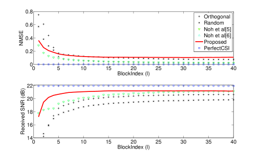
Figure 1: NMSE and received SNR versus block index $l$: $N=16$, $T_{t}=3$, $\rho/\sigma^{2}=10dB$, $\gamma=10dB$, and $v=3km/h$

Fig. 1 shows the performance of the proposed pilot design, when $\rho/\sigma^{2}=\gamma=$ 10dB and $N_{t}=16$. The normalized MSE (NMSE) is defined as $\frac{\|{\bf g}_{l}-\hat{{\bf g}}_{l|l}\|^{2}}{\|{\bf g}_{l}\|^{2}}$. The result is averaged over 100 random realizations of the channel process with length 40 blocks. For comparison, we consider orthogonal and random beam patterns for $N_{t}=16$. In addition, we consider the pilot design algorithms minimizing the channel estimation MSE in [5, 6]. It is seen that the proposed method noticeably outperforms other methods in terms of received SNR and especially yields quick convergence at the early stage of channel learning, although its MSE performance is worse than the methods in [5, 6]. Although the result is not shown here due to space limitation, it is observed in the block i.i.d. channel case that the proposed pilot design method in Section IV-A yields slightly better performance than the method in [13] in terms of received SNR.

VI Conclusion

In this paper, we have considered the pilot signal design for massive MIMO systems to maximize the received SNR under the block Gauss-Markov and block i.i.d. channel models. We have shown that the proposed design method yields noticeably better performance in terms of received SNR than channel estimation MSE-based methods. Furthermore, we have shown that using the $T_{t}$ dominant eigen-vectors of the channel covariance matrix without mixing as the pilot signal provides an optimal solution even for received SNR maximization under the block i.i.d. channel model. The extension to the MIMO case is left as future work.

References

• [1] F. Rusek, D. Persson, B. K. Lau, E. G. Larsson, O. Edfors, F. Tufvesson, and T. L. Marzetta, “Scaling up MIMO: Opportunities and challenges with very large arrays,” IEEE Signal Process. Mag., vol. 30, pp. 40 - 60, Jan., 2013.
• [2] T. L. Marzetta, “Noncooperative cellular wireless with unlimited numbers of base station antennas,” IEEE Trans. Wireless Commun., vol. 9, pp. 3590 - 3600, Nov. 2010.
• [3] J. Hoydis, S. ten Brink, and M. Debbah, “Massive MIMO in the UL/DL of cellular networks: How many antennas do we need?,” IEEE J. Sel. Areas Commun., vol. 31, pp. 160 - 171, Feb. 2013.
• [4] C. Shepard, H. Yu, N. Anand, L. E. Li, T. L. Marzetta, R. Yang, and L. Zhong, “Argos: Practical many-antenna base stations,” in Proc. MobiCom, (Istanbul, Turkey), Aug. 2012.
• [5] S. Noh, M. D. Zoltowski, Y. Sung, and D. J. Love, “Pilot beam pattern design for channel estimation in massive MIMO systems,” to appear in IEEE J. Sel. Topics Signal Process., Oct. 2014 (available at IEEExplore).
• [6] S. Noh, M. D. Zoltowski, Y. Sung, and D. J. Love, “Tranining signal design for channel estimation in massive MIMO systems,” in Proc. ICASSP (to appear), (Florence, Italy), May. 2014.
• [7] J. Choi, D. J. Love, and P. Bidigare, “Downlink training techniques for FDD massive MIMO systems: Open-loop and closed-loop training with memory,” to appear in IEEE J. Sel. Topics Signal Process., Oct. 2014 (available at IEEExplore).
• [8] B. Hassibi and B. M. Hochwald, “How much training is needed in multiple-antenna wireless links?,” IEEE Trans. Inf. Theory, vol. 49, pp. 951 - 963, Apr. 2003.
• [9] D. J. Love, J. Choi, and P. Bidigare, “A closed-loop training approach for massive MIMO beamforming systems,” in Proc. IEEE CISS, (Johns Hopkins Univ., Maryland), Mar. 2013.
• [10] S. Noh, M. D. Zoltowski, Y. Sung, and D. J. Love, “Optimal pilot beam pattern design for massive MIMO systems,” in Proc. Asilomar, (Pacific Grove, CA), Nov. 2013.
• [11] S. Stein, “Fading channel issues in system engineering,” IEEE J. Sel. Areas Commun., vol. 5, pp. 68 - 89, Feb. 1987.
• [12] A. F. Molish, Wireless Communications. New York, NY: Wiley, 2010.
• [13] J. H. Kotecha, and A. M. Sayeed, “Transmit signal design for optimal estimation of correlated MIMO channels,” IEEE Trans. Signal Process.,, vol. 52, pp. 546 - 557, Feb. 2004.
• [14] T. Kailath, A. H. Sayed, and B. Hassibi, Linear Estimation. Upper Saddle River, New Jersey: Prentice-Hall, 2000.
• [15] Z. Luo, W. Ma, A. M. So, Y. Ye, and S. Zhang, “Semidefinite relaxation of quadratic optimization problems,” IEEE Signal Process. Mag., vol. 27, pp. 20 - 34, May. 2010.
• [16] W. C. Jakes, Microwave Mobile Communication. New York, NY: Wiley, 1974.