Displacement effect in strong-field atomic ionization by an XUV pulse

Abstract

We study strong-field atomic ionization driven by an XUV pulse with a nonzero displacement, the quantity defined as the integral of the pulse vector potential taken over the pulse duration. We demonstrate that the use of such pulses may lead to an extreme sensitivity of the ionization process to subtle changes of the parameters of a driving XUV pulse, in particular, the ramp-on/off profile and the carrier envelope phase. We illustrate this sensitivity for atomic hydrogen and lithium driven by few-femtosecond XUV pulses with intensity in the $\rm 10^{14}~{}W/cm^{2}$ range. We argue that the observed effect is general and should modify strong-field ionization of any atom, provided the ionization rate is sufficiently high.

Over the past decade, it has become possible to generate short and intense pulses of coherent eXtreme UltraViolet (XUV) radiation. Sub-femtosecond XUV pulses from high-order harmonic generation (HHG) sources Goulielmakis et al. (2008); Sansone et al. (2006) have been widely used for time-resolved studies of atomic photoionization in attosecond streaking Schultze et al. (2010) and interferometric Klünder et al. (2011) experiments. Few to tens of femtosecond pulses from free-electron lasers (FEL) Ackermann et al. (2007); Shintake et al. (2008) have been instrumental for studying complex dynamics governing both sequential and direct multiple ionization processes Feldhaus et al. (2013).

There are certain peculiarities of the photoionization process in this short-wavelength intense-field regime. A nonresonant radiation field of high intensity can dress the single-electron continuum states, resulting in a distorted multi-peak structure of the photoelectron spectra Demekhin and Cederbaum (2012a). The multi-peaked spectra are typically explained in terms of the dressed-state picture Armstrong and O’Neil (1980); Cohen-Tannoudji et al. (2004), or by dynamical interference in the emission process through the interplay between the photoionization and the AC Stark shift Demekhin and Cederbaum (2012b).

In this Letter, we report yet another peculiarity of strong-field atomic ionization. Under a certain condition, the photoionization process becomes extremely sensitive to subtle changes of the driving XUV pulse such as the ramp-on/off profile and the carrier envelope phase (CEP). This condition can be formulated as a nonzero net displacement of the free electron, originally at rest, observed after the end of the pulse. This displacement can be expressed as the integral of the pulse vector potential calculated over the pulse duration. [We assume that the vector potential is zero before and after the pulse.] For nonzero displacement, we show that seemingly insignificant changes of the pulse parameters may have a dramatic effect on the photoelectron spectrum and the photoelectron angular distribution (PAD).

We explain this effect within the Kramers-Henneberger (KH) picture of the ionization process, in which the so-called “KH atom” is moving in the reference frame of the ionized electron. The ionic potential seen by the photoelectron in this frame and averaged over its oscillations, known as the KH potential, is distinctly different from the original atomic potential but still capable of supporting infinitely many bound states. These bound states can be imaged by photoelectron spectroscopy and are responsible for unexpected stabilization of atomic ionization by intense IR laser pulses Morales et al. (2011). In the present case, a hardly noticeable change of the ramp on/off profile from linear to sine-squared of a long flat-top pulse results in dramatically different KH potentials. This, in turn, alters significantly the entire photoionization process, thus resulting in a strong variation of the photoelectron spectrum as well as the PAD.

To our knowledge, little attention has been paid to date to strong-field ionization driven by the pulses with a nonzero displacement. About 20 years ago, the possibility of using such pulses was discussed Nefedov (1994), but this work has never been followed through. In this Letter, we study ionization driven by such pulses for realistic scenarios and suggest a specific recipe for possible experimental tests.

We illustrate the ramp-on/off and CEP effects for hydrogen and lithium atoms driven by $\sim$10 femtosecond pulses with peak intensity in the $\rm 10^{14}~{}W/cm^{2}$ range. Even though we use specific XUV pulse parameters, the predicted effects appear to be general and should modify strong-field ionization of any atom, including resonant photoionization, provided the ionization rate is sufficiently high. All examples presented in this Letter are for linearly polarized electric field pulses along the $\hat{\boldsymbol{z}}$ direction, with the amplitude given by $E(t)=F(t)\sin(\omega t+\delta)$, where $F(t)$ is the envelope function, $\omega$ is the central frequency, and the CEP $\delta$ is usually (except for one case) chosen as zero.

We describe the photoionization process by the nonrelativistic time-dependent Schrödinger equation (TDSE), which can be solved to a very high degree of accuracy. We restrict ourselves to the dipole approximation, ignoring any nondipole, including magnetic field, effects. This is well justified for the chosen pulse parameters. As shown in Kylstra et al. (2000), the degree of adiabaticity of the laser-atom interaction does not modify significantly the breakdown of the dipole approximation. Furthermore, the criterion $F_{0}/c\,\omega^{3}\ll 1$ Kylstra et al. (2000) , where $F_{0}$ is the field amplitude and $c$ is the speed of light, is very well fulfilled in our calculations. The latter condition corresponds to a displacement of the electron due to the magnetic field by much less than the size of the initial wave packet.

For the numerical treatment, we employed either the length or velocity gauge of the electric dipole operator and three time-propagation schemes (Crank-Nicolson Crank and Nicolson (1996), matrix iteration Nurhuda and Faisal (1999), and short iterative Lanczos Park and Light (1986)). All these schemes and gauges produced essentially identical (within the thickness of the lines) results. Exhaustive tests were performed to ensure numerical stability with respect to the space and time grids, as well as the number of partial waves coupled in the solution of the TDSE. In case of hydrogen, this stability and accuracy were used to calibrate experimental laser parameters such as the absolute intensity at the 1% level Pullen et al. (2013); Graydon (2013). In case of lithium, a very accurate theoretical description of the experimental strong field ionization spectra was achieved Schuricke et al. (2011).

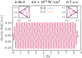
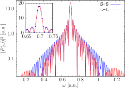
Figure 1: (Color online) Electric field (top) and Fourier spectrum (bottom) of 2-36-2 L-L and S-S pulses with central photon energy 0.7 a.u. and peak intensity of $4.0\times 10^{14}~{}$W/cm². The inserts in the top panel magnify the changes due to the small differences in the ramp-on/off cycles. The pulses are identical in the plateau regime. The L-L pulse in the bottom panel exhibits the higher side maxima. The insert (solid circles are used for the S-S pulse to make it visible) shows that the center of the frequency spectrum is virtually identical for the two cases.

As a convenient numerical example, we consider the electric field pulse with envelope functions of trapezoidal (linear ramp-on/off) shape and sine-squared shape. Both functions have the numerical advantage that they start at true zero and can also be switched off completely within a finite (not necessarily integer) number of cycles. In addition, an extended plateau in the envelope function characterizes the amplitude of the electric field.

Figure 1 shows an example of two pulses, which we will denote by “2-36-2 S-S” and “2-36-2 L-L”, respectively. Here “$n_{1}$-$n_{2}$-$n_{3}$” refers to the number of cycles in the ramp-on ($n_{1}$), the plateau ($n_{2}$), and the ramp-off ($n_{3}$), while “S” and “L” label sine-squared (S) or linear (L) ramp-on/off. In this particular example, the peak intensity is $4.0\times 10^{14}~{}$W/cm², corresponding to a peak electric field amplitude of 0.107 atomic units (a.u.). The central photon energy is 19 eV (0.7 a.u.). A similar pulse was studied recently in the context of testing numerical approaches Tetchou Nganso et al. (2011); Grum-Grzhimailo et al. (2013), except that the central photon frequency was chosen to coincide with the nonrelativistic $1s$-$2p$ resonance transition energy in what is expected to be predominantly a two-photon process. We chose a nonresonant frequency significantly larger than the field-free ionization potential in the present work, in order to avoid the impression that the effects discussed below are limited to particular resonant cases.

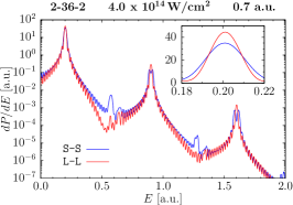
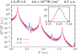
Figure 2: (Color online) Ejected-electron energy spectrum for 2-36-2 and 1.5-37-1.5 pulses with central photon energy 0.7 a.u. and peak intensity of $4.0\times 10^{14}~{}$W/cm². For visibility, dots were used for the S-S results in the lower insert.

While the well-known multi-photon character in the ejected-electron energy spectrum displayed on a logarithmic scale in Fig. 2 may not look peculiar at all, the insets show that the ramp-on/off effect can be substantial. Not only does it depend on the small difference in how the pulse is switched on and off within a given number of optical cycles (o.c.), but also on how many cycles are taken for the on/off steps. Specifically, the dominant single-photon peak displayed in the insets changes its height and width when comparing the two 2-36-2 pulses, while virtually no difference occurs for 1.5-37-1.5. Other peaks at higher photoelectron energies, corresponding to absorption of two and three photons, are split into doublets. Space does not allow for more examples here, which we refer to future publications. These results may seem surprising, as both the L-L and S-S pulses have very similar spectral content (cf. bottom panel of Fig. 1) and the phase of the Fourier decomposition (not shown).

Further analysis revealed that not only the angle-integrated spectra are very sensitive to the ramp-on/off. The partial-wave decomposition of the ionization probability, for example, and the evolution of the expectation value $\langle L^{2}\rangle$ as function of time, are completely different for 2-36-2 S-S and 2-36-2 L-L pulses. This is shown in Fig. 3. While the $\langle L^{2}\rangle$ expectation value in the presence of the laser pulse is not a directly observable quantity (it is not gauge invariant, but the right panel of Fig. 3 illustrates its evolution if the velocity gauge is employed), the marked difference in its behavior for 2-36-2 S-S and 2-36-2 L-L suggests that the quantum evolution of the system proceeds very differently in these two cases. We also see that changing the CEP of the S-S pulse can change the picture substantially. In fact, a CEP of 90^∘ makes the 2-36-2 S-S pulse look “normal” again.

The partial-wave ($\ell$) decomposition of the ionization probability (cf. Fig. 3), when computed after the end of the pulse, is another gauge-invariant parameter that can be used to check the partial-wave convergence of a calculation. In practice, the related PAD is measured experimentally, but we first look at the $\ell$-decomposition.

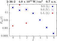
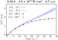
Figure 3: (Color online) Left: Angular-momentum composition of the ejected electron wave function after exposure to a 2-36-2 pulse with central photon energy 0.7 a.u. and peak intensity of $4.0\times 10^{14}~{}$W/cm². Note the broad distribution for the 2-36-2 S-S pulse and the excellent agreement between the numerical predictions obtained by independent computer codes in the length and velocity gauges. Right: Quantum mechanical expectation value of $\langle L^{2}\rangle$, as a function of time, for CPEs of $0^{\circ}$ and $90^{\circ}$.

While the distribution is sharply peaked at $\ell=1$ for the 2-36-2 L-L pulse, as one would expect for a one-photon process, Fig. 3 shows that it is broadly spread out for the 2-36-2 S-S pulse. As demonstrated in Fig. 4, the effect is, indeed, observable if the PAD is measured with an asymmetric energy window around the central peak. Such windows are typically set in experiments with reaction microscopes Ullrich et al. (2003). As seen in Fig. 4, the PADs obtained by integrating differential angle- and energy-resolved ionization probabilities over the energy interval 0.15 a.u. $\leq E\leq 0.2$ a.u. differ dramatically.

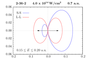
Figure 4: (Color online) PADs for the 2-36-2 S-S (blue solid line) and 2-36-2 L-L (red dashed line) pulse, integrated over the energy interval 0.15-0.2 a.u. The arrow indicates the direction of the laser polarization axis.

To explain these findings, we resort to the KH picture of the ionization process Kramers (1956); Henneberger (1968). The Hamiltonian operators in the KH gauge and the velocity gauge are related by a canonical transformation generated by the operator $\hat{T}=\int_{0}^{t}\,\boldsymbol{A}(\tau)\cdot\hat{\boldsymbol{p}}\ d\tau,\$ where $\boldsymbol{A}(\tau)$ is the vector potential. This transformation yields the Hamiltonian in the KH gauge:

$$\hat{H}_{\rm KH}=e^{{\rm i}\hat{T}}\hat{H}_{\rm V}e^{-{\rm i}\hat{T}}-{\partial\hat{T}\over\partial t}={\hat{\boldsymbol{p}}^{2}\over 2}+V(\boldsymbol{r}+\boldsymbol{x}(t))\,,$$ (1)

where $\boldsymbol{x}(t)=\int_{0}^{t}{\boldsymbol{A}}(\tau)\,d\tau$, and $V(\boldsymbol{r})$ is the potential energy in the atomic field-free Hamiltonian displaced by $\boldsymbol{x}(t)$, which is determined by the classical trajectory launched with initial zero coordinate and velocity in a linearly polarized laser field along the $\hat{\boldsymbol{z}}$ direction. For this geometry $\boldsymbol{x}(t)=Z_{\rm cl}(t)\hat{\boldsymbol{x}}$. The quantity $Z_{\rm cl}(t)$ is exhibited on the left panel of Fig. 5 for various pulses. We see that it is very different for the 2-36-2 S-S pulse compared to the 2-36-2 L-L pulse or either one of the 1.5-37-1.5 pulses.

Different behaviour of $\boldsymbol{x}(t)$ leads to different Hamiltonians in the KH picture. This difference can be illustrated by the so-called KH potential defined as

$$V_{KH}(\boldsymbol{r})={1\over T_{1}}\int\limits_{0}^{T_{1}}V(\boldsymbol{r}+\boldsymbol{x}(t))\,dt,$$ (2)

where $T_{1}$ is the total pulse duration. The KH potential in Eq. (2) is the zero-order term in the Fourier expansion of the potential $V(\boldsymbol{r}+\boldsymbol{x}(t))$. In many cases this term alone provides enough information to understand qualitatively the effect of the laser field on a system Morales et al. (2011). If necessary, corrections to this simplified description can be generated by adding higher-order terms of the Fourier expansion. We show the KH potentials on the right panel of Fig. 5 for the 2-36-2 S-S and 2-36-2 L-L pulses. Note that the KH potential for the 2-36-2 L-L pulse is nearly Coulombic, whereas for the 2-36-2 S-S case it is strongly distorted and far away from a spherically symmetric form. This provides another explanation why the angular-momentum distributions presented above for the 2-36-2 S-S case are so broad.

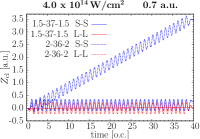
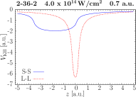
Figure 5: (Color online) Left: Classical trajectory without Coulomb field for an electron starting at the origin with zero speed under the influence of the laser field for 1.5-37-1.5 and 2-36-2 pulses with central photon energy 0.7 a.u. and peak intensity of $4.0\times 10^{14}~{}$W/cm². Right: Kramers-Henneberger potential along the line running at the distance $\rho=0.1$ a.u. parallel to the polarization axis of the laser pulse for the 2-36-2 S-S (blue) solid and 2-36-2 L-L (red) dashed lines.

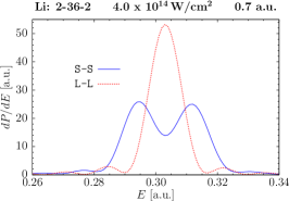
Figure 6: (Color online) Ejected electron spectrum for Li for ionization by the 2-36-2 S-S (blue) solid and 2-36-2 L-L (red) dashed lines pulses with central photon energy 0.5 a.u. and peak intensity of $4.0\times 10^{14}~{}$W/cm².

Because of its universal nature, this effect should be observable in any atom and not just be restricted to the hydrogen case chosen for illustration. Indeed, Fig. 6 displays ionization spectra for the lithium atom driven by a similar set of S-S and L-L pulses with a central frequency of 13.6 eV and peak intensity of $4.0\times 10^{14}~{}$W/cm². The ramp on/off effect in the energy spectra is very similar to that observed for the hydrogen atom. It also manifests itself in the PADs integrated over the energy interval covering approximately half of the ionization peak in Fig. 6, while it essentially disappears if a symmetric energy window is used. The latter is illustrated in Fig. 7.

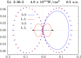
Figure 7: (Color online) PADs for Li by pulses with central photon energy 0.5 a.u. and peak intensity of $4.0\times 10^{14}~{}$W/cm². Lines are for an asymmetric energy window, 0.25 a.u.$\;\leq E\leq$0.30 a.u., while symbols are for a symmetric energy window, 0.25 a.u.$\;\leq E\leq$0.35 a.u., around the central peak. The arrow indicates the direction of the laser polarization axis.

To summarize, we have demonstrated a significant, and so far unexplored for realistic scenarios, effect of the laser pulse ramp-on/off and CEP on atomic ionization in the strong field regime when the driving XUV pulse has a nonzero displacement. We attribute this effect to small changes in the initial conditions launching significantly different classical electron trajectories. This, in turn, leads to different Kramers-Henneberger potentials experienced by the receding photoelectron and results in significantly different photoelectron spectra, angular-momentum compositions, and PADs.

We illustrated the proposed effect using specific pulse parameters that are not far from those presently available from HHG and FEL sources. Once we find a combination of the pulse parameters describing the ramp-on/off and the CEP such that the displacement has a nonzero value, we may expect a dramatic effect in the energy spectra and PADs. The stronger the field and the longer the pulse, the more visible the effect should generally be. Also, the ramp-on/off effect is very visible in resonant photoionization. We observed a strong modification of the Autler-Townes doublet in hydrogen at the resonant photon energy of 3/8 a.u. Details will be discussed in future publications.

An important issue, of course, concerns the occurrence of pulses with a nonzero displacement experimentally. To our knowledge, the existence of such pulses does not contradict Maxwell’s equations, nor any other known physical law. Rastunkov and Krainov (2007) strongly favored pulses with zero displacement, in order to prevent the electron from leaving the laser interaction region too early. In practice, however, a displacement of a few atomic units (c.f. Fig. 5) should not be unrealistic in light of the typical size of the laser focus.

In fact, the requirement that the net displacement is zero, i.e., that the integral of the vector potential over the pulse duration vanishes, is very restrictive. This constraint connects the pulse shape and its CEP, i.e., we cannot freely change one without changing the other if we want to limit the pulse to cause zero displacement. We are not aware of this restriction having ever been considered, for example, in the design or interpretation of experiments on quantum control. Theoretically at least, these parameters are varied independently.

The authors benefited greatly from many stimulating discussions with Misha Ivanov, Igor Litvinyuk, and Peter Hannaford. One of the authors (KB) wishes to thank the Australian National University for hospitality. This work was supported by the Australian Research Council under Grant No. DP120101805 (IAI and ASK), by the United States National Science Foundation under Grants No. PHY-1068140, PHY-1430245, and the XSEDE allocation PHY-090031 (KB, JE, SMB), and by the Russian Foundation for Basic Research under Grant No. 12-02-01123 (EG and ANG). Resources of the Australian National Computational Infrastructure (NCI) Facility were also employed.

References

- Goulielmakis et al. (2008) E. Goulielmakis, M. Schultze, M. Hofstetter, V. S. Yakovlev, J. Gagnon, M. Uiberacker, A. L. Aquila, E. M. Gullikson, D. T. Attwood, R. Kienberger, et al., Science 320(5883), 1614 (2008).
- Sansone et al. (2006) G. Sansone, E. Benedetti, F. Calegari, C. Vozzi, L. Avaldi, R. Flammini, L. Poletto, P. Villoresi, C. Altucci, R. Velotta, et al., Science 314(5798), 443 (2006).
- Schultze et al. (2010) M. Schultze, M. Fiess, N. Karpowicz, J. Gagnon, M. Korbman, M. Hofstetter, S. Neppl, A. L. Cavalieri, Y. Komninos, T. Mercouris, et al., Science 328(5986), 1658 (2010).
- Klünder et al. (2011) K. Klünder, J. M. Dahlström, M. Gisselbrecht, T. Fordell, M. Swoboda, D. Guénot, P. Johnsson, J. Caillat, J. Mauritsson, A. Maquet, et al., Phys. Rev. Lett. 106(14), 143002 (2011).
- Ackermann et al. (2007) W. Ackermann et al., Nat. Phot. 1, 336 (2007).
- Shintake et al. (2008) T. Shintake et al., Nat. Phot. 2, 555 (2008).
- Feldhaus et al. (2013) J. Feldhaus, M. Krikunova, M. Meyer, T. Möller, R. Moshammer, A. Rudenko, T. Tschentscher, and J. Ullrich, J. Phys. B 46(16), 164002 (2013).
- Demekhin and Cederbaum (2012a) P. V. Demekhin and L. S. Cederbaum, Phys. Rev. Lett. 108, 253001 (2012a).
- Armstrong and O’Neil (1980) L. Armstrong and S. V. O’Neil, J. Phys. B 13(6), 1125 (1980).
- Cohen-Tannoudji et al. (2004) C. Cohen-Tannoudji, J. Dupont-Roc, and G. Grynberg, Atom-Photon Interactions: Basic Processes and Applications (Willey, New-York, 2004).
- Demekhin and Cederbaum (2012b) P. V. Demekhin and L. S. Cederbaum, Phys. Rev. A 86, 063412 (2012b).
- Morales et al. (2011) F. Morales, M. Richter, S. Patchkovskii, and O. Smirnova, Proc. Natl. Acad. Sci. 108(41), 16906 (2011).
- Nefedov (1994) A. L. Nefedov, Phys. Rev. A 50, R903 (1994).
- Kylstra et al. (2000) N. Kylstra, R. A. Worthington, A. Patel, P. L. Knight, J. R. V. de Aldana, and L. Roso, Phys. Rev. Lett. 85, 1835 (2000).
- Crank and Nicolson (1996) J. Crank and P. Nicolson, Advances in Computational Mathematics 6(1), 207 (1996), ISSN 1019-7168.
- Nurhuda and Faisal (1999) M. Nurhuda and F. H. M. Faisal, Phys. Rev. A 60, 3125 (1999).
- Park and Light (1986) T. Park and J. Light, Journal of Chemical Physics 85, 5870 (1986).
- Pullen et al. (2013) M. G. Pullen, W. C. Wallace, D. E. Laban, A. J. Palmer, G. F. Hanne, A. N. Grum-Grzhimailo, K. Bartschat, I. Ivanov, A. Kheifets, D. Wells, et al., Phys. Rev. A 87, 053411 (2013).
- Graydon (2013) O. Graydon, Nat. Photon. 7, 585 (2013).
- Schuricke et al. (2011) M. Schuricke, G. Zhu, J. Steinmann, K. Simeonidis, I. Ivanov, A. Kheifets, A. N. Grum-Grzhimailo, K. Bartschat, A. Dorn, and J. Ullrich, Phys. Rev. A 83(2), 023413 (2011).
- Tetchou Nganso et al. (2011) H. M. Tetchou Nganso, Y. V. Popov, B. Piraux, J. Madroñero, and M. G. K. Njock, Phys. Rev. A 83, 013401 (2011).
- Grum-Grzhimailo et al. (2013) A. N. Grum-Grzhimailo, M. N. Khaerdinov, and K. Bartschat, Phys. Rev. A 88, 055401 (2013).
- Ullrich et al. (2003) J. Ullrich, R. Moshammer, A. Dorn, R. Dörner, L. P. H. Schmidt, and H. Schmidt-Böcking, Rep. Prog. Phys. 66(9), 1463 (2003).
- Kramers (1956) H. A. Kramers, Collected Scientific Papers (North Holland, Amsterdam, 1956).
- Henneberger (1968) W. C. Henneberger, Phys. Rev. Lett. 21, 838 (1968).
- Rastunkov and Krainov (2007) V. S. Rastunkov and V. P. Krainov, J. Phys. B 40(12), 2277 (2007).