Plasticity of hydrogen bond networks regulates mechanochemistry of cell adhesion complexes

Abstract

Mechanical forces acting on cell adhesion receptor proteins regulate a range of cellular functions by formation and rupture of non-covalent interactions with ligands. Typically, force decreases the lifetimes of intact complexes (slip-bonds), making the discovery that these lifetimes can also be prolonged (“catch-bonds”), a surprise. We created a microscopic analytic theory by incorporating the structures of selectin and integrin receptors into a conceptual framework based on the theory of stochastic equations, which quantitatively explains a wide range of experimental data (including catch-bonds at low forces and slip-bonds at high forces). Catch-bonds arise due to force-induced remodeling of hydrogen bond networks, a finding that also accounts for unbinding in structurally unrelated integrin-fibronectin and actomyosin complexes. For the selectin family, remodeling of hydrogen bond networks drives an allosteric transition resulting in the formation of maximum number of hydrogen bonds determined only by the structure of the receptor and is independent of the ligand. A similar transition allows us to predict the increase in number of hydrogen bonds in a particular allosteric state of $\alpha_{5}\beta_{1}$ integrin–fibronectin complex, a conformation which is yet to be crystallized. We also make a testable prediction that a single point mutation (Tyr51Phe) in the ligand associated with selectin should dramatically alter the nature of the catch-bond compared to the wild type. Our work suggests that nature utilizes a ductile network of hydrogen bonds to engineer function over a broad range of forces.

Significance Statement

Selectins and integrins are receptor proteins on cell surfaces responsible for adhesion to a variety of extracellular biomolecules, a critical component of physiological processes like white blood cell localization at sites of inflammation. The bonds which the receptors form with their targets are regulated by mechanical forces (for example due to blood flow). The bond lifetimes before rupture exhibit a counterintuitive increase with force, before decreasing as expected. Based on crystal structures of selectin and integrin, we created a general analytic theory which for the first time relates microscopic structural rearrangements at the receptor-ligand interface to macroscopic bond lifetimes. We quantitatively explain experimental data from diverse systems spanning four decades of lifetime scales, and also predict the outcome of mutations in specific residues.

Introduction

Cells communicate with each other and their surroundings in order to maintain tissue architecture, allow cellular movement, transduce signals and heal wounds Berrier & Yamada (2007). Important components in many of these processes are cell adhesion molecules—proteins on cell surfaces that recognize and bind to ligands on other cells or the extracellular matrix Berrier & Yamada (2007); Gumbiner (1996). For example, adhesion of leukocytes to the endothelial cells of the blood vessel is a vital step in rolling and capturing of blood cells in wound-healing, and is mediated by the selectin class of receptor proteins Ley et al. (2007). The functional responses of cell adhesion molecules are often mechanically transduced by shear stresses and forces arising from focal adhesions to the cytoskeleton or simply the flow of blood in the vasculature. Under stress, molecules undergo conformational changes, triggering biophysical, biochemical, and gene regulatory responses that have been the subject of intense research Davies (1995); Traub & Berk (1998). Lifetimes of adhesion complexes are typically expected to decrease as forces increase Bell (1978). However, the response of certain complexes to mechanical force exhibits a surprisingly counterintuitive phenomenon. Lifetimes increase over a range of low force values, corresponding to “catch-bond” behavior Dembo et al. (1988). At high forces, the lifetimes revert to the conventional decreasing behavior, characteristic of a “slip-bond” Bell (1978). In retrospect, the plausible existence of catch-bonds was already evident in early experiments by Greig and Brooks, who discovered that agglutination of human red blood cells using the lectin concanavalin A, increased under shear Greig & Brooks (1979). Although not interpreted in terms of catch-bonds, their data showed lower rates of unbinding with increasing force on the complex. Given the importance of mechanotransduction in cellular adhesions, a quantitative and structural understanding of this surprising phenomenon is imperative.

Direct evidence for catch-bonds in a wide variety of cell adhesion complexes have come from flow and AFM experiments in the last decade Thomas et al. (2002); Marshall et al. (2003); Kong et al. (2009), along with examples from other load-bearing cellular complexes like actomyosin bonds Guo & Guilford (2006) and microtubule-kinetochore attachments Akiyoshi et al. (2010). The catch-bond lifetime exhibits non-monotonic biphasic behavior—increasing up to a certain critical force and decreasing at larger forces. The structural mechanisms leading to catch-bond behavior have largely been elusive, though experiments have provided key insights for selectins Somers et al. (2000); Phan et al. (2006) and integrins Luo et al. (2007); Zhu et al. (2013). In these systems, the rupture rate of the ligand from the receptor depends on an angle between two domains in the receptor molecule (Fig. 1). Conformations with smaller angles detach more slowly than those with large angles. In the case of integrins, multiple conformations at varying angles have been crystallized Zhu et al. (2013), while for selectins, only two (see Fig. 1) have been found so far in the crystal structures Somers et al. (2000). In the absence of an external force, the molecule fluctuates between conformations corresponding to a variety of angles, including the larger angles from which the ligand can rapidly detach. With the application of force, the two domains increasingly align along the force direction, restricting the system to small angles and longer lifetimes, until large forces again reduce the barrier to rupture.

Previously, theories based on kinetic models with the assumption of a phenomenological Bell-like coupling of rates to force Evans et al. (2004); Barsegov & Thirumalai (2005); Lou et al. (2006); Pereverzev et al. (2009) have been used to explain catch-bond behavior. However, the parameters extracted from these kinetic models cannot be easily related to microscopic physical processes in specific catch-bond systems. More importantly, such models merely rationalize the experimental data, and do not have predictive power. The large scale of catch-bond lifetimes, $\sim 10-10^{4}$ ms, makes it impossible to directly observe unbinding in a realistic all-atom simulation, much less the macroscopic consequences of mutations.

Here, we solve the difficulties alluded to above by creating a new theoretical approach. By building on the insights from the structures of cell adhesion complexes, we introduce a microscopic theoretical model that captures the essential physics of the angle-dependent detachment, and its implications for catch-bond behavior. Taking cue from the crystal structures of selectin and integrin, we construct a coarse-grained energy function for receptor-ligand interactions. The model yields an analytic expression for the bond lifetime as a function of force, which gives excellent fits to a broad range of experimental data on a number of systems. The extracted parameters have clear structural interpretations, and their values provide predictions for energetic and structural features like strength of hydrogen bonding networks at the receptor-ligand interface. Where estimates of these properties can be directly obtained from crystal structures, our predictions are in remarkable agreement. The energy scales identified through the model are specific enough to allow predictions for structures not yet crystallized, and suggest novel mutation experiments that would modify catch-bond behavior in quantifiable ways. For the selectins, we predict how a specific mutation in the PSGL-1 ligand will alter its unbinding from P-selectin under force, and provide new interpretation of data from L-selectin mutants Lou et al. (2006). Interestingly, the experimental fits suggest that both P- and L-selectin have a characteristic, ligand-independent energy scale, determined by the chemistry of their binding interfaces. For integrins, we predict the strength of extra interactions that should be observed in a crystal structure of the $\alpha_{5}\beta_{1}$–fibronectin complex in an open state. The generality of the theory is further established by obtaining quantitative agreement for the catch-bond behavior in actomyosin complex. Our theory provides the first structural link between the catch to slip bond transition in cell adhesion complexes, covering a broad range of forces and lifetimes.

Theory

Structural basis of catch-bond model: We now define our model using the structures of P-selectin, which has been crystallized in two conformations: a “bent” [Fig. 1a] and “extended” state [Fig. 1b] Somers et al. (2000). The two states differ by the angle which the EGF domain (green in Figs. 1a and 1b) assumes with respect to the lectin domain (gray/beige). Although ligands can bind to lectin in both conformations, co-crystallization with the ligand (the truncated N-terminal portion of the glycoprotein PSGL-1) was achieved only for the extended state. In this latter case, there are two major regions of the lectin domain (B₀ and B₁, colored purple in Figs. 1a - 1d) that form substantial hydrogen bond networks with the ligand, thereby stabilizing the complex. Based on alignments of the lectin domain in the bent and extended states [Fig. 2a], it is believed that the binding interface is remodeled in the bent conformation Somers et al. (2000); Springer (2009). The region B₁ (a loop between Asp82 and Glu88, shown in the inset of Fig. 2a) rotates so that it can no longer engage the ligand. This angle-dependent rearrangement results in weaker ligand attachment, and hence explains the shorter bond lifetimes in the bent vs. the extended conformation.

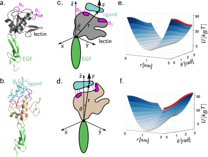
Figure 1: Abstraction of the model based on structure. a. Crystal structure of P-selectin Somers et al. (2000) in the bent conformation (PDB: 1G1Q); b. the extended conformation (PDB: 1G1S). The lectin (gray/beige) and EGF (green) domains are labeled, along with two regions of the ligand binding interface (B₀ and B₁, purple). The ligand (an N-terminal fragment of the glycoprotein PSGL-1) is only co-crystallized in the extended state. c-d. Schematic conformations of our model, corresponding to panels a and b. e-f. Plots of the potential $U(r,\theta)$ at $F=0$ and $F=50$pN respectively, with $k_{0}=80\,k_{B}T/\text{nm}^{2}$, $k_{1}=20\,k_{B}T/\text{nm}^{2}$, $r_{0}=1.0\,\text{nm}$, and $b=2$ nm. The energy $U(b,\theta)$ at the transition state is highlighted in red.

Our minimal model, which captures the structure based angle-dependent dissociation, describes the ligand-receptor interaction through an effective spring with bond vector $\mathbf{r}\equiv\left(r,\theta,\phi\right)$ between a pivot point within the receptor and a point in the ligand [Fig. 1c-d]. The pivot point is fixed at the origin, and the ligand is under an external force $F\hat{\mathbf{z}}$ along the $z$-axis. The energy associated with the spring is given by the potential,

$$U(r,\theta)=\frac{1}{2}\left(k_{0}+k_{1}(1+\cos\theta)\right)(r-r_{0})^{2}-Fr\cos\theta,$$ (1)

with $k_{0},k_{1}>0$. The first term is an elastic energy, where $r_{0}$ is the natural length of the bond magnitude $r$, and $k_{0}+k_{1}(1+\cos\theta)\equiv k(\theta)$ is an angle-dependent spring constant. The second term is the contribution due to the mechanical force $F$. The bond ruptures if $r\geq b$, where $b\equiv r_{0}+d$ and $d$ is the transition state distance. The structural inspiration of our model naturally leads to a multidimensional potential energy, dependent on both $r$ and $\theta$, which is a key requirement for a physically sensible description of catch-bond behavior. Any one-dimensional potential with rupture defined by a single cutoff in some reaction coordinate will always exhibit monotonic lifetime behavior as a function of force. We assume that the time evolution of the vector $\mathbf{r}$ follows a Fokker-Planck equation, describing diffusion on the potential surface $U(r,\theta)$ with a diffusion constant $D$. We define the lifetime of the bond $\tau(F)$ at a given force $F$ as the mean first passage time from $\mathbf{r}_{\text{min}}(F)$, the position of the minimum in $U$, to any $\mathbf{r}$ with $r=b$. Implicit in this diffusive picture is the assumption that the angle $\theta$ can change continuously. This is a reasonable approximation even if the receptor-ligand complex fluctuates between several discrete angular states Zhu et al. (2013), assuming the energy barriers between the states are such that the interconversion between states happens on much faster timescales than $\tau(F)$. The presence of the barriers would in this case be incorporated through a renormalization of the effective diffusion constant $D$ Zwanzig (1988).

We show in Fig. 1e a representative zero-force potential energy surface $U(r,\theta)$, with the energy at rupture $U(b,\theta)$, highlighted in red. The form of $k(\theta)$ makes it energetically favorable for bond rupture at $\theta=\pi$ (the bent state), with a cost $E_{0}=k_{0}d^{2}/2$ to dislodge the ligand to the failure point. In the opposite limit of $\theta=0$ (the extended state), energy for rupture is highest, with a cost $E_{0}+E_{1}$, where $E_{1}=k_{1}d^{2}$. The values of $E_{0}$ and $E_{1}$ correspond to the stabilization energies associated with the ligand in the two allosteric (bent and extended) states. However, as $F$ is increased, the bond aligns along $\hat{\mathbf{z}}$, and the minimum in $U(r,\theta)$ shifts toward $\theta=0$ [Fig. 1f], biasing the system toward the extended state. Thus, we expect the lifetime $\tau(F)$ to initially increase with $F$ and eventually decrease at forces sufficiently large to reduce the rupture barrier.

Though the schematic diagram of the model in Fig. 1c-d draws the vector $\mathbf{r}$ between a pivot at the EGF-lectin interface to the tip of the ligand, one should note that the actual ligand-lectin complex does not behave like a perfectly rigid object rotating about a hinge, nor does it cover the entire angular range between $\theta=0$ and $\pi$. Since proteins are deformable, the pivot location and the length $r_{0}$ will depend on the compliance of the specific domains involved in reorientation. Hence, we expect $r_{0}$ to be of the order of, or less than the size of the localized domains that rotate to become restructured under force. It therefore follows that the structures of the complex in different allosteric states provide valuable insights into their response to force. The length scale $d$ reflects the brittleness of the bonding interactions Hyeon & Thirumalai (2007), with larger $d$ indicating a malleable bond interface which can be deformed over longer distances before the complex falls apart. The two energy scales $E_{0}$ and $E_{1}$ also have physical interpretations, with $E_{0}$ being roughly the total strength of noncovalent interactions between the region $B_{0}$ and the ligand, whereas $E_{1}$ is the additional contribution from the region $B_{1}$ in the extended conformation.

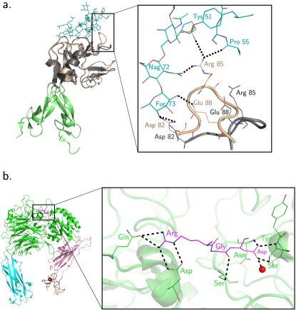
Figure 2: Receptor–ligand hydrogen bond networks in P-selectin and $\alpha_{5}\beta_{1}$ integrin. a. The crystal structures from Fig. 1a,b superimposed with aligned lectin domains. The inset shows the remodeling of the $B_{1}$ region of the ligand-binding interface (the Asp82–Glu88 loop). In the extended state (beige) this loop forms a network of hydrogen bonds (dashed lines) with the ligand (to be compared with $E_{1}$ of our model). In the bent state (gray) the loop rotates sufficiently far that it is unlikely to participate in binding Somers et al. (2000); Springer (2009). b. Hydrogen bond network between ligand RGD and $\alpha_{5}\beta_{1}$ integrin in the closed headpiece conformation (PDB: 3VI4). The integrin domains are colored as follows: $\beta$-propeller and $\beta$A in green (cartoon and line representation), thigh in cyan, hybrid in pink and PSI in brown. The ligand is colored magenta (stick or line) and the MIDAS magnesium ion is red (sphere). This network should be compared to $E_{0}$, predicted from our model.

Results and Discussion

Mean bond lifetime: By assuming that $\tau(F)$ is much longer than the local equilibration time around $\mathbf{r}_{\text{min}}(F)$, the lifetime of the complex is approximately given by,

$$\tau(F)\approx\frac{\sqrt{\pi}\,r_{0}(E_{1}-2F(d+r_{0}))e^{\beta(E_{0}+dF)}(e^{2\beta Fr_{0}}-1)}{4D(\beta E_{0})^{3/2}F\left(1+r_{0}/d\right)^{2}(1-e^{\beta(2F(d+r_{0})-E_{1})})},$$ (2)

where $\beta=1/k_{B}T$, $k_{B}$ is the Boltzmann constant, and $T$ is the temperature. The full details of the derivation are in the SI. The central result of this work in Eq. (S2) provides an analytic expression for the mean first passage time in terms of the microscopic energy and length scales covering both the catch and slip-bond regimes. To set a reasonable scale for $D$, we make it equal to the diffusivity of a sphere of radius $r_{0}$, $D=k_{B}T/6\pi\eta r_{0}$, where $\eta$ is the viscosity of water. (A prefactor in $D$ due to molecular shape can be absorbed as a small logarithmic correction to the energy scale $E_{0}$.) With this assumption, Eq. (S2) becomes an equation with four parameters: $E_{0}$, $E_{1}$, $d$ and $r_{0}$. We validated the approximation underlying Eq. (S2) by comparison to Brownian dynamics simulations of diffusion on $U$ (details in the SI), which showed excellent agreement with our analytical theory (see Fig. S2 in the SI).

For $\beta Fd\gg 1$, $\tau(F)$ decays exponentially in a manner similar to the standard Bell model for systems exhibiting slip-bonds, $\tau(F)\sim\exp(-\beta dF)$. The decay rate is controlled by the transition state distance $d$. The characteristic catch-bond behavior occurs at smaller $F$, where we see a biphasic $\tau(F)$ peaked at $F=F_{\text{p}}$,

$$F_{\text{p}}\approx\frac{AE_{1}}{2(r_{0}+d)},$$ (3)

with a prefactor $A\sim{\cal O}(1)$. The ratio of the peak height $\tau(F_{\text{p}})$ to the lifetime $\tau(0)$ at zero force, which is a measure of the strength of the catch-bond, scales like

$$\frac{\tau(F_{\text{p}})}{\tau(0)}\approx\frac{4A^{\prime}(d+r_{0})}{r_{0}E_{1}^{2}}\sinh\left(\frac{E_{1}}{2}\right)\sinh\left(\frac{r_{0}E_{1}}{2(d+r_{0})}\right),$$ (4)

with a prefactor $A^{\prime}\sim{\cal O}(1)$. From Eqs. (S3) and (S4) we see that $E_{1}\to 0$ leads to $F_{\text{p}}\to 0$ and $\tau(F_{\text{p}})/\tau(0)\to 1$. In this limit, the model predicts only slip-bond behavior, where the lifetime decreases monotonically with force. Thus, our model interpolates between catch-bond and slip-bond regimes by varying the energy scale $E_{1}$.

Analysis of experimental data: We first establish the efficacy of the theory by analyzing experimental data for $\tau(F)$ for a variety of complexes. The fits in Fig. 3 (selectins) and Fig. 4 (non-selectin complexes) show that there is excellent agreement between the analytical theory and measurements, which is remarkable since our microscopic model shows that only a small number of fitting parameters suffice to fit nine complexes with vastly differing architectures. These experiments involve applying force to molecular complexes either through AFM or optical traps, with the force initially ramped from zero to a given value $F$. Bonds which survive the ramp are then held at constant $F$ until rupture. If the initial ramp is sufficiently slow such that the system always remains quasi-adiabatically in equilibrium at the instantaneous applied force Raible et al. (2004), the subsequent duration of the bond while at constant $F$, averaged over many trials, provides an accurate estimate of $\tau(F)$. (Extremely high ramp speeds may lead to non-equilibrium artifacts Sarangapani et al. (2011).)

In order to establish that our theory is general, we analyzed experimental results from both selectin systems (P-selectin Marshall et al. (2003), L-selectin Lou et al. (2006)), and others (fibronectin disassociating from a truncated construct of $\alpha_{5}\beta_{1}$ integrin Kong et al. (2009) and myosin unbinding from actin Guo & Guilford (2006)). Details of the maximum-likelihood procedure for obtaining the best-fit parameter values (Table I) are in the SI. All the systems in Figs. 3 and 4 exhibit catch-bonds at low forces except in Fig. 3b, which for comparison shows P-selectin forming a slip-bond ($E_{1}=0$) with the antibody G1.

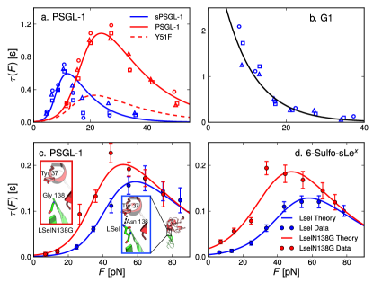
Figure 3: Experimental best-fit results for bond lifetime $\tau(F)$ versus force $F$ for selectins. The top and bottom rows correspond to the receptors P-selectin (Psel) and L-selectin (Lsel) respectively. The ligands are indicated above the figures. The symbols are experimental results and the lines are analytical curves from Eq. (S2), with parameters given in Table I. The sources for the data are: a-b) Marshall et al. (2003); c-d) Lou et al. (2006). For panels a-b, the symbol shapes denote three alternate ways of estimating experimental $\tau(F)$. Squares: average of the lifetimes; triangles: standard deviation of the lifetimes; circles: -1/slope in the logarithmic plot of the number of events with lifetime $t$ or more versus $t$. Up to sampling errors, these estimates are equivalent for systems with exponentially distributed bond lifetimes.

Selectin family: Fig. 3a includes data for P-selectin with two different forms of PSGL-1 ligand: sPSGL-1, which is a monomer interacting with single lectin domains, and PSGL-1, which is a dimer capable of simultaneously forming two bonds with two neighboring lectin domains Marshall et al. (2003). (All other selectin complexes, including L-selectin / PSGL-1 Lou et al. (2006) in Fig. 3c-d, involve only monomeric interactions.) We fit both curves in Fig. 3a with the same set of parameters, using $\tau(F)$ from Eq. (S2) for the monomeric case, and in the dimer case $\tau_{\text{dim}}(F)\equiv\tau(F/2)+\tau(F/2)[1+k_{r}\tau(F/2)]/2$ Marshall et al. (2003). When the dimer is intact, each bond feels a force $F/2$. When one of the bonds break, the intact bond still feels a force approximately equal to $F/2$, due to the large stiffness and roughly constant displacement of the AFM cantilever Pereverzev et al. (2005). In the latter case, the broken bond can reform with some rate $k_{r}$, which adds one fitting parameter. $\tau_{\text{dim}}(F)$ is a model that accounts for all these possibilities. The resulting fits in Fig. 3a show that a total of five parameters ($k_{r}\approx 1.1\pm 0.3$ s^-1, the rest listed in Table I) can simultaneously capture the general lifetime behaviors of both data sets.

Physical meaning of the parameters: A sine qua non of a valid theory of any phenomenon is that the extracted parameters must have sound physical meaning. In order to provide a structural interpretation of the extracted parameters for the selectin systems, it is instructive to compare the resulting energy and length scales to what we know about selectin bonds independent of the model. From the crystal structure of the P-selectin / PSGL-1 complex in Fig. 1b, we estimated that the regions B₀ and B₁ involve, respectively, 14 and 6 ligand-lectin hydrogen bonds (the B₁ bonds are shown in Fig. 2a). We used the software PyMol Schrödinger (2010) to count hydrogen bonds, with a distance cutoff of $0.35$ nm for the heavy atoms. The corresponding energy scales from Table I are $E_{0}=17$ $k_{B}T$ and $E_{1}=9$ $k_{B}T$, which gives an enthalpy of $\approx 1.2-1.5$ $k_{B}T$ per hydrogen bond. This range is consistent with earlier estimates of the strength of hydrogen bonds in proteins Bolen & Rose (2008). The distance from the EGF domain–lectin interface to the lectin–ligand interface is $\approx 3$ nm. Since the crystal structures suggest that restructuring of hydrogen bonds in this region leads to catch-bond behavior, $r_{0}$ should be $\approx 3$ nm or less. The fitted values of $r_{0}\approx 0.2-2.0$ nm for L- and P-selectin, lie well within this estimate. The transition distances $d$ vary between $\approx 0.1-0.6$ nm, which is the range typical for proteins Elms et al. (2012). Given the realistic values for all the fitted parameters, our theoretical model is an accurate coarse-grained description of selectin-type systems.

The sum $E_{0}+E_{1}$ is essentially constant for a given selectin receptor, independent of the ligand: $E_{0}+E_{1}\approx 27\>k_{B}T$ for P-selectin and $\approx 31\>k_{B}T$ for L-selectin. This suggests that the maximum number of possible interactions is fixed by the interactions associated with the receptor interface. For each ligand there is a different partitioning of these interactions among those that contribute to $E_{0}$ and $E_{1}$. The values of $E_{0}$ and $E_{1}$ can be estimated from the structures alone using $E_{0}\approx n_{b}\epsilon_{hb}$ and $E_{0}+E_{1}\approx n_{e}\epsilon_{hb}$ where $n_{b}$, $n_{e}$ are the number of hydrogen bonds in the bent and extended states respectively and $\epsilon_{hb}$ is the strength of a hydrogen bond. For the catch-bond complexes, $E_{1}\approx 7-10$ $k_{B}T$, or roughly 5-8 noncovalent bonds. For P-selectin and G1 [Fig. 3b], all interactions contribute to $E_{0}$, and we get slip-bond behavior instead; G1 is a blocking monoclonal antibody for P-selectin. In this case the binding is so strong, involving all possible interactions at the interface, that there is no room for additional stabilization under alignment ($E_{1}=0$). The finding that the ligands achieve nearly the same value of $E_{0}+E_{1}$ means that in the aligned state each of the considered ligands is capable of maximally exploiting the binding partners among the receptor residues. Our model predicts that if the ligand were made defective, by truncating or mutating some portion of the ligand binding sites so that their interactions with the receptor were eliminated, the sum $E_{0}+E_{1}$ should decrease. We will return to this case below in discussing a mutant of the ligand PSGL-1.

Table 1: Best-fit parameter values of the catch-bond model for the various experimental complexes shown in Figs. 3-4. Parentheses denote uncertainties in the least significant digit.

Complex	$E_{1}$	$E_{0}$	$d$	$r_{0}$
	[$k_{B}T$]	[$k_{B}T$]	[nm]	[nm]
Psel / (s)PSGL-1	$9.3(2)$	$17.2(3)$	$0.56(2)$	$2.0(1)$
Psel / G1	$0$	$26.73(4)$	$0.51(3)$	$2.0$ a
Lsel / PSGL-1	10.2(7)	20.3(6)	0.14(4)	0.38(7)
LselN138G / PSGL-1	8.7(6)	21.8(5)	0.14(4)	0.38(7)
Lsel / $\text{6-sulfo-sLe}^{\text{x}}$	8.7(7)	22.7(4)	0.17(4)	0.23(5)
LselN138G / $\text{6-sulfo-sLe}^{\text{x}}$	7.0(7)	24.3(3)	0.17(4)	0.23(5)
integrin / fibronectin	$12(1)$	$23(1)$	$0.7(1)$	$0.5(2)$
actin / myosin (ADP)	$4.1(3)$	$18.2(5)$	$0.47(4)$	$2.6(5)$
actin / myosin (rigor)	$3.9(4)$	$18.4(8)$	$0.50(5)$	$2.2(7)$

^a For this Psel slip-bond system, the lack of data at small forces prevents independent fitting of $r_{0}$, so its value is set to the $r_{0}$ result for Psel/(s)PSGL-1.

Integrin: In the case of the integrin-fibronectin complex, we took as an example AFM data for a truncated integrin (only the headpiece of $\alpha_{5}\beta_{1}$) binding to fibronectin FNIII_7-10 (fibronectin fragment comprising the 7-10th type III repeats) Kong et al. (2009). There is ample evidence for an angle-dependent detachment of ligand in the integrin headpiece Luo et al. (2007), where the $\beta$-hybrid domain swings out from the $\alpha$ subunit via multiple intermediate states Zhu et al. (2013). Our model is well suited to describe these structural changes, and the quality of fit to experimental data [Fig. 4a] shows that the physics governing the effect of force on selectin complexes also holds for the complex involving integrin. We can compare some of the fitted parameters with a recently obtained crystal structure of the $\alpha_{5}\beta_{1}$ headpiece complexed with fibronectin (only the RGD peptide portion of fibronectin is resolved in the structure, Fig. 2b) Nagae et al. (2012).

Since the structure shows the integrin headpiece in a closed (large angle) conformation, we can directly compare the number of hydrogen bonds with the parameter $E_{0}$. As shown in Fig. 2b, there are nine hydrogen bonds formed between the headpiece domain and the RGD peptide. In addition, the acidic residue Asp forms a salt-bridge with the ligand residue Arg. Beyond the interactions that can be ascertained from the crystal structure, it is also known that additional “synergy” sites in the ligand, not visible in the structure, play a role in binding. From the measured decrease in binding affinity of fibronectin fragments lacking the synergy sites, their contribution to the binding energy can be estimated to be $\approx 2-4$ $k_{B}T$ Nagae et al. (2012). Combining this with the hydrogen bonds and salt bridges seen in the structure (using our earlier range of $1.2-1.5$ $k_{B}T$ per hydrogen bond, and $4-8$ $k_{B}T$ for the salt bridge Gohlke & Klebe (2002)) we get an estimated total of $E_{0}=(17-26)$ $k_{B}T$. Our fitted result $E_{0}=23$ $k_{B}T$ from the model falls in this range, and is therefore consistent with the structural analysis. The fitted value of $r_{0}$ is also reasonable, given that the longest axis of the hybrid domain is $\sim 4$ nm. The parameter $d$ is again well within the range of transition state distances expected in proteins. Our model predicts that $E_{1}=12$ $k_{B}T$, the extra interaction strength that would be gained in an open conformation of the $\alpha_{5}\beta_{1}$–fibronectin complex. This prediction can be verified once crystal structures of the open conformation become available.

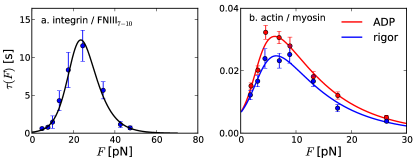
Figure 4: Experimental best-fit results for bond lifetime $\tau(F)$ for non-selectin complexes. The receptor ligand systems are indicated on top of the figures. Sources of the data are a. Kong et al. (2009) and b. Guo & Guilford (2006).

Actomyosin: Finally, in the case of actomyosin catch-bonds [Fig. 4b], no crystal structures exist for the complex and an angle-dependent lifetime has not been established. However, we can use our theory to propose the origins of catch-bond behavior in these complexes based on experimental data. There is strong evidence that the upper 50K and lower 50K domains surrounding the major cleft in the motor head behave like pincers—binding to actin tightly in the ADP and rigor states, thereby forming a tight complex Holmes et al. (2003). Once ATP binds, the pincers move apart (the upper 50K domain breaks contact with actin) by an allosteric mechanism Tehver & Thirumalai (2010), thus allowing the motor head to unbind from actin faster. While in the ADP/rigor state, if an external force is applied through the lever arms of myosin, local rearrangements and rotations would cause the N terminal domain and the two 50K domains to align with the direction of force. Along with these local reorientations, the force would also stretch the domains, causing narrowing of the major cleft, and facilitating increased interactions of both 50K domains with actin. This mechanism would lead to catch-bond behavior, in a manner similar to the FimH-mannose adhesions in E. Coli Le Trong et al. (2010). Our fitted value of $r_{0}$ shows that the alignments occur over a length-scale $\sim 2.4$ nm, which agrees well with single molecule results showing that the cross-bridge compliance resides only locally in the actin-motor domain of the actomyosin complex Molloy et al. (1995).

Predictions for mutations in selectin complexes: Since the energy scales in our model correspond to the strengths of noncovalent bonding networks, we can use our theory to predict and explain the impact of mutations on the bond lifetime, thus providing a framework for engineering catch-bonds with specific properties. We will consider two examples, one a modification of the ligand, the other of the receptor in selectin systems. A recent study Xiao et al. (2012) considered a PSGL-1 mutant where Tys51, a sulfated tyrosine that makes one hydrogen bond with Arg85 in the B₁ region of P-selectin [Fig. 2], is replaced by phenylalanine (Phe), which cannot form the hydrogen bond. Kinetic assays showed that the mutant has a weaker binding affinity to P-selectin, but a zero force off-rate that remains virtually unchanged from the wild-type. The lifetime under force has not yet been measured, but our model predicts that removing one hydrogen bond from B₁ should decrease $E_{1}$ by $\approx 1.3$ $k_{B}T$. Using the reduced value for $E_{1}$ with all other parameters the same as in the wild-type (first row of Table I), we predict that the $\tau(F)$ curve (dashed red line labeled Y51F in Fig. 3a), should be dramatically different from the wild-type. Relative to the wild-type, the peak is decreased by a factor of 3.4, and shifted slightly (from 24 to 21 pN). Since effects of a mutation in $E_{1}$ are most relevant to alignment under force, the low force behavior is relatively unperturbed, similar to the kinetic assay results: $\tau(F)$ of the mutant for $F<2$ pN differs less than 20% from the wild-type.

The second example, where experimental $\tau(F)$ data is available, involves two receptor mutations performed on L-selectin Lou et al. (2006). The authors compared the $\tau(F)$ behavior of wild-type L-selectin to a mutant where Asn138 was changed to Gly. The mutation effectively breaks a hydrogen bond in the hinge region, between Tyr37 and Asn138. Two different ligands (PSGL-1 and 6-sulfo-sLe${}^{\text{x}}$) both showed the same trends: the peak in the $\tau(F)$ curve for the mutant was shifted up and toward smaller forces, relative to the wild-type [Fig. 3c-d]. To determine the minimal perturbation in the parameters that would produce this shift, we simultaneously fit the wild-type and mutant data sets for each ligand, allowing only a subset of parameters to change for the mutant. The most likely subset, determined using the Akaike information criterion (see SI for details), involved only changes in the energy scales $E_{0}$ and $E_{1}$. The fit results are shown in Table I. Both ligands show a similar pattern: $E_{1}$ decreased by $\approx 1.5-1.7$ $k_{B}T$ in the mutant, while $E_{0}$ increased by $\approx 1.5-1.6$ $k_{B}T$. The magnitudes of the energy changes suggest that the enthalpy loss due to a single hydrogen bond contributing to $E_{1}$ in the wild-type is compensated by an increase in $E_{0}$. The mutation gives added flexibility to the lectin domain, allowing it to bind the ligand more effectively in both the bent and extended conformations. Thus, a contact between the ligand and receptor in $B_{1}$ [Fig. 1] that forms only at small angles in the wild-type, is present at all angles in the mutant.

Conclusions

The general principle for the formation of catch-bonds emerging from experiments and theory is an increase in stabilizing interactions as a result of topological rearrangements of protein domains under force Barsegov & Thirumalai (2005); Springer (2009). While we quantitatively establish the mechanism for certain classes of protein complexes in this work, recent computational studies on a knotted protein Sulkowska et al. (2009) and a long $\alpha$ helix Kreuzer et al. (2013) suggest that the same principle could lead to non-monotonic unfolding lifetimes in single proteins as well. In the former, the protein thymidine kinase was studied, where a “threaded” loop is surrounded by a “knotting” loop, forming a slip-knot Sulkowska et al. (2009). At intermediate forces, the knotting loop shrinks faster than the threaded loop, effectively leading to increased interactions between the loops and hence an increased barrier to unfolding. At smaller forces, the threaded loop shrinks faster and slips out of the knotting loop, before any extra interactions can form. In the beta-myosin helix studied using molecular simulations with the milestoning algorithm Kreuzer et al. (2013), at intermediate forces broken hydrogen bonds from the native alpha helix secondary structure reform to create a longer-lived force-stabilized pi helix structure, thereby leading to a catch-bond like effect. More generally, we suggest that if the number of hydrogen bond or side chain interactions can be increased in single domain proteins by force-induced structural rearrangements then such systems should exhibit catch bond behavior. This is likely to be the case in mammalian prions which have a number of unsatisfied hydrogen bonds in the functional state Dima & Thirumalai (2002). Thus, it is increasingly becoming clear that diverse force-induced topological rearrangements can be used by nature as a mechanism to modulate bond lifetimes.

At the larger scale of protein complexes, one can ask whether the rearrangements responsible for catch-bonds among different biomolecule families share common features. From structure-based observations in selectin and integrin systems, we have shown that a model based on force dependent rotation of protein domains, facilitating enhanced interactions with their binding partner, explains experimental observations remarkably well. Our precise analytical theory quantitatively reproduces data on a variety of structurally unrelated complexes with lifetimes spanning nearly four orders of magnitude. More importantly, the key parameters of the theory are linked to the formation (or disruption) of a network of hydrogen bonds and/or salt-bridges. Because the strength of these interactions can be estimated, our theory can be readily used to predict the effects of mutations, as demonstrated for the selectin complexes. Interestingly, analysis of experimental data allowed us to predict the strength of additional hydrogen bonds that form in the open $\alpha_{5}\beta_{1}$ integrin–fibronectin complex. The specificity of our model, with very few parameters, lays a foundation for synthetic mechanochemistry Konda et al. (2013): designing and fine-tuning catch-bond adhesion complexes with a desired set of load-bearing characteristics.

Acknowledgements: This work was supported by a grant from the National Institutes of Health through grant number GM 089685.

Supplementary Information for:
Plasticity of hydrogen bond networks regulates mechanochemistry of cell adhesion complexes
Shaon Chakrabarti, Michael Hinczewski, and D. Thirumalai

I Derivation of the equation for bond lifetime

The dynamics of our model can be described by the probability density $\Psi(\mathbf{r},t)$ to find the system with bond vector $\mathbf{r}=(r,\theta,\phi)$ at time $t$. This probability evolves according to the Fokker-Planck equation in spherical coordinates,

$$\begin{split}\frac{\partial\Psi}{\partial t}=&\frac{D}{r^{2}}\frac{\partial}{\partial r}\left[r^{2}e^{-\beta U}\frac{\partial{\left(e^{\beta U}\Psi\right)}}{\partial{r}}\right]+\frac{D}{r^{2}\sin\theta}\frac{\partial}{\partial\theta}\left[\sin\theta e^{-\beta U}\frac{\partial{\left(e^{\beta U}\Psi\right)}}{\partial{\theta}}\right]\\ &+\frac{D}{r^{2}\text{sin}^{2}\theta}\frac{\partial}{\partial{\phi}}\left[e^{-\beta U}\frac{\partial{\left(e^{\beta U}\Psi\right)}}{\partial{\phi}}\right],\end{split}$$ (S1)

with $\beta=1/k_{B}T$. Eq. (S1) describes diffusion on the energy surface $U(r,\theta)$,

$$U(r,\theta)=\frac{1}{2}\left(k_{0}+k_{1}(1+\cos\theta)\right)(r-r_{0})^{2}-Fr\cos\theta,$$ (S2)

with diffusion constant $D$. We define the marginal probability $P(r,\theta,t)$ by multiplying $\Psi$ with the spherical Jacobian and integrating over the azimuthal angle $\phi$,

$$P(r,\theta,t)\equiv r^{2}\sin\theta\int_{0}^{2\pi}d\phi\Psi(\mathbf{r},t).$$ (S3)

Since $U$ is independent of $\phi$, carrying out the operation in Eq. (S3) and using Eq. (S1) leads to a two-dimensional Fokker-Planck equation for $P(r,\theta,t)$,

$$\frac{\partial P}{\partial t}=D\frac{\partial}{\partial{r}}\left[e^{-\beta V}\frac{\partial{\left(e^{\beta V}P\right)}}{\partial{r}}\right]+\frac{D}{r^{2}}\frac{\partial}{\partial{\theta}}\left[e^{-\beta V}\frac{\partial{\left(e^{\beta V}P\right)}}{\partial{\theta}}\right],$$ (S4)

in terms of a modified potential

$$V(r,\theta)=U(r,\theta)-k_{B}T\log(r^{2}\sin\theta).$$ (S5)

For a given force $F$, we are interested in the mean first passage time (MFPT) $\tau_{0}(r,\theta,F)$ from a point $(r,\theta)$ with $r<b$ to any point $(b,\theta^{\prime})$ at the boundary defining bond rupture. The MFPT satisfies the following equation Kampen (2007), derived from the backward Fokker-Planck equation,

$$D\frac{\partial}{\partial r}\left[e^{-\beta V}\frac{\partial\tau_{0}}{\partial r}\right]+\frac{D}{r^{2}}\frac{\partial}{\partial\theta}\left[e^{-\beta V}\frac{\partial\tau_{0}}{\partial\theta}\right]=-e^{-\beta V},$$ (S6)

with boundary condition $\tau_{0}(b,\theta^{\prime},F)=0$ for all $\theta^{\prime}$. Since the two-dimensional first-passage problem in Eq. (S6) cannot be solved analytically, we will approximately map it to a one-dimensional problem. Integrating Eq. (S6) over $\theta$ leads to

$$D\frac{\partial}{\partial r}\int_{0}^{\pi}d\theta\,e^{-\beta V(r,\theta)}\frac{\partial}{\partial r}\tau_{0}(r,\theta,F)=-\int_{0}^{\pi}d\theta\,e^{-\beta V(r,\theta)}.$$ (S7)

The second term in Eq. (S6) vanishes under the integration because $\exp(-\beta V(r,\theta))\to 0$ in the limits $\theta\to 0^{+}$ and $\theta\to\pi^{-}$, as can be seen from Eq. (S5).

In order to evaluate the integral on the left hand side of Eq. (S7) we make a saddle-point approximation, replacing $\partial\tau_{0}(r,\theta,F)/\partial r$ with, $\partial\tau_{0}(r,\theta_{\text{m}}(r),F)/\partial r$, where $\theta_{\text{m}}(r)$ is the location of the minimum of $V(r,\theta)$ at a fixed radius $r$. For our potential, a single such minimum exists for any given $r$, making $\theta_{\text{m}}(r)$ a well-defined function. The result is an approximate one-dimensional MFPT equation,

$$D\frac{\partial}{\partial r}\left[e^{-\beta\tilde{V}(r)}\frac{\partial}{\partial r}\tilde{\tau}_{0}(r,F)\right]=-e^{-\beta\tilde{V}(r)},$$ (S8)

where $\tilde{\tau}_{0}(r,F)\equiv\tau_{0}(r,\theta_{\text{m}}(r),F)$ and the effective one-dimensional potential $\tilde{V}(r)$ is given by

$$\tilde{V}(r)\equiv-\frac{1}{\beta}\log\int_{0}^{\pi}d\theta\,e^{-\beta V(r,\theta)}=-\frac{1}{\beta}\log\left[\frac{r^{2}e^{-\beta(Fr+\frac{1}{2}k_{0}(r-r_{0})^{2})}\left(e^{2\beta(Fr-\frac{1}{2}k_{1}(r-r_{0})^{2})}-1\right)}{\beta(Fr-\frac{1}{2}k_{1}(r-r_{0})^{2})}\right].$$ (S9)

With the boundary condition $\tilde{\tau}_{0}(b,F)=0$, Eq. (S8) can be solved for $\tilde{\tau}_{0}(r,F)$,

$$\tilde{\tau}_{0}(r,F)=\frac{1}{D}\int_{r}^{b}dr^{\prime}\,e^{\beta\tilde{V}(r^{\prime})}\int_{0}^{r^{\prime}}dr^{\prime\prime}e^{-\beta\tilde{V}(r^{\prime\prime})}.$$ (S10)

The function $\tilde{V}(r^{\prime})$ is a monotonically increasing function of $r^{\prime}$ at large $r^{\prime}$. Hence the integral over $r^{\prime}$ in Eq. (S10) gets its dominant contribution from $r^{\prime}$ near the upper limit $b$, due to the presence of the $\exp(\beta\tilde{V}(r^{\prime}))$ term. To simplify the integral, we will make two approximations: (i) Expand $\tilde{V}(r^{\prime})\approx\tilde{V}(b)+\tilde{V}^{\prime}(b)(r^{\prime}-b)$. (ii) Assume $b\gg r_{\text{m}}$, where $r_{\text{m}}$ is the location of the minimum in $\tilde{V}(r)$, so that the upper limit in the inner integral over $r^{\prime\prime}$ can be replaced by $\infty$. If the initial position $r$ is close to the potential minimum at $r_{\text{m}}$, so that $b\gg r$, the integrals in Eq. (S10) can be then approximately carried out to yield

$$\tilde{\tau}_{0}(r,F)\approx\frac{e^{\beta\tilde{V}(b)}}{\beta D\tilde{V}^{\prime}(b)}\int_{0}^{\infty}dr^{\prime\prime}\,e^{-\beta\tilde{V}(r^{\prime\prime})}=\left[D\tilde{P}^{\prime}(b)\right]^{-1},$$ (S11)

where

$$\tilde{P}(r)\equiv{\tilde{Z}}^{-1}e^{-\beta\tilde{V}(r)},\quad\tilde{Z}\equiv\int_{0}^{\infty}dr^{\prime}\,e^{-\beta\tilde{V}(r^{\prime})}.$$ (S12)

Since under this approximation $\tilde{\tau}_{0}(r,F)$ is independent of the starting point $r$, we will drop the $r$ dependence, and simplify the notation by defining the approximate bond lifetime $\tau(F)\equiv\tilde{\tau}_{0}(r,F)$.

To obtain an analytical expression for $\tau(F)$, we need to evaluate the integral for $\tilde{Z}$ in Eq. (S12) for $\tilde{P}(r)$. Since this cannot be done exactly, we will approximate $\tilde{Z}$ as a Gaussian integral by expanding $\tilde{V}(r)$ around $r=r_{\text{m}}$ to second order, leading to

$$\tilde{Z}\approx\left(\frac{\beta\tilde{V}^{\prime\prime}(r_{\text{m}})}{2\pi}\right)^{-1}e^{-\beta\tilde{V}(r_{\text{m}})}.$$ (S13)

To find closed-form expressions for $r_{\text{m}}$ and the $\tilde{V}^{\prime\prime}(r_{\text{m}})$, we note that the location of the minimum of $\tilde{V}(r)$ and the curvature at the minimum approximately coincide with those of the simpler potential $\tilde{V}_{\text{s}}(r)$,

$$\tilde{V}_{\text{s}}(r)=\frac{1}{2}\left(k_{0}+2k_{1}\right)(r-r_{0})^{2}-Fr-2k_{b}T\log r,$$ (S14)

which comes from substituting $\cos(\theta)\to 1$ in $V(r,\theta)$ in the integral defining $\tilde{V}(r)$ [Eq. (S9)]. Fig. S1 illustrates $\tilde{V}(r)$ versus $\tilde{V}_{\text{s}}(r)$ at two

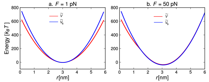
Figure S1: Comparison of the potentials $\tilde{V}(r)$ and $\tilde{V}_{\text{s}}(r)$ at two different forces: a) $F=1$ pN; b) $F=50$ pN. The energy scales are aligned such that the minima of both potentials occur at $0$ $k_{B}T$. The parameters are: $k_{0}=147.2\>k_{B}T/\text{nm}^{2}$, $k_{1}=15.6\>k_{B}T/\text{nm}^{2}$, $r_{0}=3.0$ nm.

different $F$. Obtaining the location and curvature of the minimum using the simple potential $\tilde{V}_{\text{s}}(r)$ is justified because of the following observations: The exact location of the minimum $r_{\text{m}}$, is always very close to $r_{0}$. At zero external force or forces very close to zero, $V(r,\theta)$ is approximately the same as the simpler potential obtained by setting $\cos(\theta)\to 1$ in $V(r,\theta)$, in regions $r\sim r_{0}$. Hence, $\tilde{V}(r)$ and $\tilde{V}_{\text{s}}(r)$ will be similar around $r=r_{0}$. At larger forces, $V(r,\theta)$ and its simpler version are approximately the same only around $r\sim r_{0}$ and $\theta\sim 0$. However, since $V(r,\theta)$ is minimized around $\theta\sim 0$ in regions around $r_{0}$, the dominant contribution to the integral in Eq. (S9) for $r$ values around $r_{0}$ comes from $\theta\sim 0$. Hence once again the simpler form of $V(r,\theta)$ can be used leading to similar $\tilde{V}(r)$ and $\tilde{V}_{\text{s}}(r)$ around $r=r_{0}$. The potential $\tilde{V}_{\text{s}}(r)$ reaches its minimum at

$$r_{\text{ms}}=4\left[-\beta(F+(k_{0}+2k_{1})r_{0})+\sqrt{8\beta(k_{0}+2k_{1})+\beta^{2}(F+(k_{0}+2k_{1})r_{0})^{2}}\right]^{-1},$$ (S15)

where the curvature is given by

$$\tilde{V}^{\prime\prime}_{\text{s}}(r_{\text{ms}})=k_{0}+2k_{1}+\frac{2}{\beta r_{\text{ms}}^{2}}.$$ (S16)

The complete approximation for $\tilde{Z}$ involves substituting Eqs. (S15) and (S16) for $r_{\text{m}}$ and $\tilde{V}^{\prime\prime}(r_{\text{m}})$ in Eq. (S13),

$$\tilde{Z}\approx\left(\frac{\beta\tilde{V}^{\prime\prime}_{\text{s}}(r_{\text{ms}})}{2\pi}\right)^{-1}e^{-\beta\tilde{V}(r_{\text{ms}})}.$$ (S17)

Plugging the definition of $\tilde{V}(r)$ from Eq. (S9) and $\tilde{Z}$ from Eq. (S17) into Eq. (S12) for $\tilde{P}(r)$, we can now analytically approximate $\tau(F)=[D\tilde{P}^{\prime}(b)]^{-1}$. The resulting expression simplifies for large $k_{0}$, corresponding to large energy barriers for bond rupture, yielding the final form for the bond lifetime [Eq. (2) of the main text],

$$\tau(F)\approx\frac{\sqrt{\pi}\,r_{0}(E_{1}-2F(d+r_{0}))e^{\beta(E_{0}+dF)}(e^{2\beta Fr_{0}}-1)}{4D(\beta E_{0})^{3/2}F\left(1+r_{0}/d\right)^{2}(1-e^{\beta(2F(d+r_{0})-E_{1})})},$$ (S18)

where $E_{0}=k_{0}d^{2}/2$ and $E_{1}=k_{1}d^{2}$.

II Brownian Dynamics Simulations

To check the accuracy of the theoretical prediction for the lifetime $\tau(F)$ in Eq. (S18), we performed overdamped Brownian dynamics simulations Ermak & McCammon (1978) for a test particle of radius $r_{0}$ diffusing in the potential $U$ given in Eq. (S2) using $D=k_{B}T/(6\pi\eta r_{0})$, where $\eta=0.89$ mPa$\cdot$s is the viscosity of water at $T=298$ K. We chose the time step for numerical integration to be about $2\times 10^{-6}r_{0}^{2}/D$. The trajectories were started with the bead at $\mathbf{r}_{\text{min}}$, the minimum of the potential $U$, and stopped when the bead reached the rupture boundary at $r=b$ for the first time. Statistics were obtained from $\approx 150-300$ trajectories, depending on the value of force, and error bars on the simulated data were estimated by the jackknife method Miller (1974). Fig. S2 shows a comparison of the numerical results to the analytical formula of Eq. (S18) for parameters corresponding to the rigor actomyosin experimental system (main text Table I). The excellent agreement validates the approximations used to derive Eq. (S18).

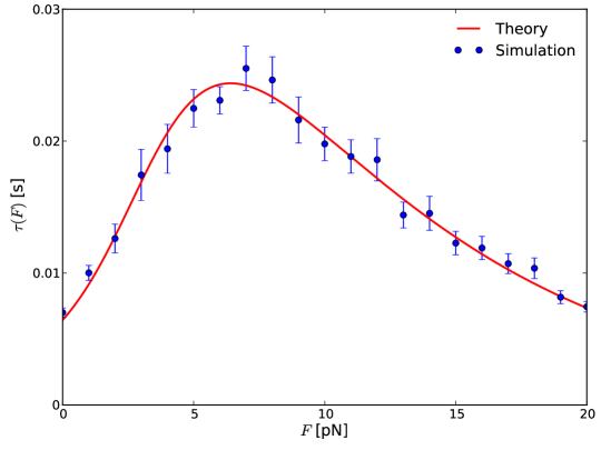
Figure S2: Approximate theoretical bond lifetime $\tau(F)$ [Eq. (S18), solid curve] versus the numerical results of Brownian dynamics simulation (circles), for parameters: $E_{0}=18.4$ $k_{B}T$, $E_{1}=3.9$ $k_{B}T$, $d=0.5$ nm, $r_{0}=2.2$ nm.

III Fitting to Experimental Data

We fitted Eq. (S18) for $\tau(F)$ to experimental data by the standard method of minimizing $\chi^{2}$ values, which is equivalent to maximizing a log-likelihood function, with the assumption that errors in the mean lifetime data are Gaussian-distributed. For the fits in Fig. 3c-d and Fig. 4 of the main text, the standard deviation for each lifetime was obtained from the error bars given in the corresponding experimental studies. However, since error bars were not provided for the lifetime data in Fig. 3a-b, we derived error bars from the scatter in the three reported estimates for $\tau(F)$: average lifetimes, standard deviation of the lifetimes, and -1/slope in the logarithmic plot of the number of events with lifetime $t$ or greater versus $t$. For exponentially distributed lifetimes (the case in all the experimental systems under consideration), these three quantities should be equal to $\tau(F)$ up to deviations due to sampling errors. After fitting, the uncertainties in the parameters $E_{0}$, $E_{1}$, $d$, and $r_{0}$ listed in Table I of the main text were obtained from the diagonal elements of the best-fit covariance matrix.

For the simultaneous fitting of L-selectin mutation data Lou et al. (2006) in Fig. 3c-d of the main text, we used the following procedure to determine the minimal perturbation to the parameters of the system that produces the observed shift in the $\tau(F)$ curves. The data alone suggests that not all the model parameters are relevant to the mutation. The experimental $\tau(F)$ curves for the wild-type (WT) and the mutant in Fig. 3c-d show that the decay in $\tau(F)$ at large $F$ is similar. Since the decay is controlled by the parameter $d$, we assume that the value of $d$ for the WT and the mutant is the same. This leaves three parameters, $E_{0}$, $E_{1}$, $r_{0}$, that could potentially be altered by the mutation, though it is possible that only a subset of these is sufficient to explain the shift. We carried out simultaneous fitting of the model to the WT and mutant $\tau(F)$ curves for each ligand, under eight different hypotheses, corresponding to different subsets of the three parameters varying under mutation. For a given ligand, the mutant and WT share all parameters except the subset that is allowed to vary (first column of Table S1). Between curves for different ligands, all parameters are distinct. The table shows the resulting $\chi^{2}$ statistic (the total $\chi^{2}$ for the data sets involving both ligands). The lowest $\chi^{2}$ is achieved for hypothesis 3, where all three parameters are allowed to vary. However, this could be the result of overfitting, since hypothesis 3 also has the largest number of free parameters. A better way to rank the hypotheses is through the corrected Akaike information criterion,

$$\text{AICc}=\chi^{2}+2p+\frac{2p(p+1)}{n-p-1},$$ (S19)

where $n$ is the number of data points and $p$ the number of free parameters Burnham & Anderson (2002). The AICc penalizes overfitting due to an excessive number of parameters, and has a natural probabilistic interpretation: if two model fits have AICc values of $a_{1}$ and $a_{2}$ respectively, with $a_{1}<a_{2}$, then model 2 has a likelihood $\exp((a_{1}-a_{2})/2)$ of being the true interpretation of the data, relative to model 1. From AICc values listed in Table S1, we see that the most likely hypothesis is 1, where $E_{0}$ and $E_{1}$ are allowed to vary. Hypothesis 2 ($E_{1}$ and $r_{0}$ varying) is a close competitor (78% as likely as 1), and the remaining ones are increasingly improbable (hypothesis 3 is only 3% as likely as 1). As argued in the main text, hypothesis 1 also has a very reasonable physical interpretation, with the mutation causing a single bond to switch between the sets that contribute to $E_{1}$ and $E_{0}$. Hypothesis 2, which involves the mutation decreasing $E_{1}$ and increasing the lever arm distance $r_{0}$, is more difficult to explain in physical terms, but cannot be completely ruled out based on fitting alone. The fit results for hypothesis 1 are shown in Fig. 3c-d, and the parameters are listed in Table I of the main text.

Table S2: Simultaneous fitting of the L-selectin mutation data [4]. The first column lists eight hypotheses, corresponding to different subsets of parameters that are allowed to vary between the fits to the wild-type and mutant data sets. $\chi^{2}$ is a measure of goodness of fit, and AICc is the corrected Akaike criterion. The hypotheses are ordered by increasing AICc.The lowest values of $\chi^{2}$ and AICc are in bold.

Varying subset	$\chi^{2}$	AICc
1: $E_{0}$, $E_{1}$	32.2	71.8
2: $E_{1}$, $r_{0}$	32.7	72.3
3: $E_{0}$, $E_{1}$, $r_{0}$	27.3	78.7
4: $E_{0}$, $r_{0}$	50.9	90.5
5: $r_{0}$	65.9	95.9
6: $E_{0}$	90.8	120.8
7: $E_{1}$	154.0	184.0
8: none	224.1	246.0

References

- Berrier & Yamada (2007) Berrier, A. L. & Yamada, K. M. Cell-matrix adhesion. J. Cell. Physiol. 213, 565–573 (2007).
- Gumbiner (1996) Gumbiner, B. M. Cell adhesion: the molecular basis of tissue architecture and morphogenesis. Cell 84, 345–357 (1996).
- Ley et al. (2007) Ley, K., Laudanna, C., Cybulsky, M. I. & Nourshargh, S. Getting to the site of inflammation: the leukocyte adhesion cascade updated. Nat. Rev. Immunol. 7, 678–689 (2007).
- Davies (1995) Davies, P. F. Flow-mediated endothelial mechanotransduction. Physiol. Rev. 75, 519–560 (1995).
- Traub & Berk (1998) Traub, O. & Berk, B. C. Laminar Shear Stress Mechanisms by Which Endothelial Cells Transduce an Atheroprotective Force. Arterioscler Thromb Vasc Biol 18, 677–685 (1998).
- Bell (1978) Bell, G. I. Models for the specific adhesion of cells to cells. Science 200, 618–627 (1978).
- Dembo et al. (1988) Dembo, M., Torney, D. C., Saxman, K. & Hammer, D. The reaction-limited kinetics of membrane-to-surface adhesion and detachment. Proc. R. Soc. Lond., B, Biol. Sci. 234, 55–83 (1988).
- Greig & Brooks (1979) Greig, R. G. & Brooks, D. E. Shear-induced concanavalin A agglutination of human erythrocytes. Nature 282, 738–739 (1979).
- Thomas et al. (2002) Thomas, W. E., Trintchina, E., Forero, M., Vogel, V. & Sokurenko, E. V. Bacterial Adhesion to Target Cells Enhanced by Shear Force. Cell 109, 913–923 (2002).
- Marshall et al. (2003) Marshall, B. T. et al. Direct observation of catch bonds involving cell-adhesion molecules. Nature 423, 190–193 (2003).
- Kong et al. (2009) Kong, F., Garc a, A. J., Mould, A. P., Humphries, M. J. & Zhu, C. Demonstration of catch bonds between an integrin and its ligand. J Cell Biol 185, 1275–1284 (2009).
- Guo & Guilford (2006) Guo, B. & Guilford, W. H. Mechanics of actomyosin bonds in different nucleotide states are tuned to muscle contraction. Proc. Natl. Acad. Sci. 103, 9844–9849 (2006).
- Akiyoshi et al. (2010) Akiyoshi, B. et al. Tension directly stabilizes reconstituted kinetochore-microtubule attachments. Nature 468, 576–579 (2010).
- Somers et al. (2000) Somers, W. S., Tang, J., Shaw, G. D. & Camphausen, R. T. Insights into the molecular basis of leukocyte tethering and rolling revealed by structures of P- and E-selectin bound to SLe(X) and PSGL-1. Cell 103, 467–479 (2000).
- Phan et al. (2006) Phan, U. T., Waldron, T. T. & Springer, T. A. Remodeling of the lectin EGF-like domain interface in P- and L- selectin increases adhesiveness and shear resistance under hydrodynamic force. Nat. Immunol. 7, 883–889 (2006).
- Luo et al. (2007) Luo, B.-H., Carman, C. V. & Springer, T. A. Structural basis of integrin regulation and signaling. Annu. Rev. Immunol. 25, 619–647 (2007).
- Zhu et al. (2013) Zhu, J., Zhu, J. & Springer, T. A. Complete integrin headpiece opening in eight steps. J. Cell Biol. 201, 1053–1068 (2013).
- Evans et al. (2004) Evans, E., Leung, A., Heinrich, V. & Zhu, C. Mechanical switching and coupling between two dissociation pathways in a P-selectin adhesion bond. Proc. Natl. Acad. Sci. 101, 11281–11286 (2004).
- Barsegov & Thirumalai (2005) Barsegov, V. & Thirumalai, D. Dynamics of unbinding of cell adhesion molecules: Transition from catch to slip bonds. Proc. Natl. Acad. Sci. 102, 1835–1839 (2005).
- Lou et al. (2006) Lou, J. et al. Flow-enhanced adhesion regulated by a selectin interdomain hinge. J. Cell Biol. 174, 1107–1117 (2006).
- Pereverzev et al. (2009) Pereverzev, Y. V., Prezhdo, O. V. & Sokurenko, E. V. Phys. Rev. E 79, 051913 (2009).
- Springer (2009) Springer, T. A. Structural basis for selectin mechanochemistry. Proc. Natl. Acad. Sci. U.S.A. 106, 91–96 (2009).
- Zwanzig (1988) Zwanzig, R. Diffusion in a rough potential. Proc. Natl. Acad. Sci. 85, 2029–2030 (1988).
- Hyeon & Thirumalai (2007) Hyeon, C. & Thirumalai, D. Measuring the energy landscape roughness and the transition state location of biomolecules using single molecule mechanical unfolding experiments. J. Phys.: Condens. Matter 19, 113101 (2007).
- Raible et al. (2004) Raible, M., Evstigneev, M., Reimann, P., Bartels, F. & Ros, R. Theoretical analysis of dynamic force spectroscopy experiments on ligand receptor complexes. J. Biotech. 112, 13–23 (2004).
- Sarangapani et al. (2011) Sarangapani, K. K. et al. Regulation of catch bonds by rate of force application. J. Biol. Chem. 286, 32749–32761 (2011).
- Pereverzev et al. (2005) Pereverzev, Y. V., Prezhdo, O. V., Forero, M., Sokurenko, E. V. & Thomas, W. E. The Two-Pathway Model for the Catch-Slip Transition in Biological Adhesion. Biophys. J. 89, 1446–1454 (2005).
- Schrödinger (2010) Schrödinger, L. The PyMOL Molecular Graphics System, Version 1.3r1 (2010).
- Bolen & Rose (2008) Bolen, D. W. & Rose, G. D. Structure and Energetics of the Hydrogen-Bonded Backbone in Protein Folding. Annu. Rev. Biochem. 77, 339–362 (2008).
- Elms et al. (2012) Elms, P. J., Chodera, J. D., Bustamante, C. & Marqusee, S. The molten globule state is unusually deformable under mechanical force. Proc. Natl. Acad. Sci. USA 109, 3796–3801 (2012).
- Nagae et al. (2012) Nagae, M. et al. Crystal structure of integrin ectodomain: Atomic details of the fibronectin receptor. J Cell Biol 197, 131–140 (2012).
- Gohlke & Klebe (2002) Gohlke, H. & Klebe, G. Approaches to the description and prediction of the binding affinity of small-molecule ligands to macromolecular receptors. Angew. Chem. Int. Ed. 41, 2644–2676 (2002).
- Holmes et al. (2003) Holmes, K. C., Angert, I., Kull, F. J., Jahn, W. & Schröder, R. R. Electron cryo-microscopy shows how strong binding of myosin to actin releases nucleotide. Nature 425, 423–427 (2003).
- Tehver & Thirumalai (2010) Tehver, R. & Thirumalai, D. Rigor to Post-Rigor Transition in Myosin V: Link between the Dynamics and the Supporting Architecture. Structure 18, 471–481 (2010).
- Le Trong et al. (2010) Le Trong, I. et al. Structural basis for mechanical force regulation of the adhesin FimH via finger trap-like beta sheet twisting. Cell 141, 645–655 (2010).
- Molloy et al. (1995) Molloy, J. E. et al. Single-molecule mechanics of heavy meromyosin and S1 interacting with rabbit or Drosophila actins using optical tweezers. Biophys. J. 68, 298S–303S; 303S–305S (1995).
- Xiao et al. (2012) Xiao, B. et al. Tyrosine Replacement of PSGL-1 Reduces Association Kinetics with P- and L-Selectin on the Cell Membrane. Biophys. J. 103, 777–785 (2012).
- Sulkowska et al. (2009) Sulkowska, J. I., Sulkowski, P. & Onuchic, J. N. Jamming Proteins with Slipknots and Their Free Energy Landscape. Phys. Rev. Lett. 103, 268103 (2009).
- Kreuzer et al. (2013) Kreuzer, S. M., Moon, T. J. & Elber, R. Catch bond-like kinetics of helix cracking: Network analysis by molecular dynamics and Milestoning. The Journal of Chemical Physics 139, 121902 (2013).
- Dima & Thirumalai (2002) Dima, R. I. & Thirumalai, D. Exploring the propensities of helices in PrPC to form sheet using NMR structures and sequence alignments. Biophys. J. 83, 1268–1280 (2002).
- Konda et al. (2013) Konda, S. S. M. et al. Molecular Catch Bonds and the Anti-Hammond Effect in Polymer Mechanochemistry. J. Am. Chem. Soc. 135, 12722–12729 (2013).

References

- Kampen (2007) Kampen, N. G. v. Stochastic processes in physics and chemistry (Elsevier, Amsterdam, 2007).
- Ermak & McCammon (1978) Ermak, D. L. & McCammon, J. A. Brownian dynamics with hydrodynamic interactions. J. Chem. Phys. 69, 1352–1360 (1978).
- Miller (1974) Miller, R. G. Jackknife - review. Biometrika 61, 1–15 (1974).
- Lou et al. (2006) Lou, J. et al. Flow-enhanced adhesion regulated by a selectin interdomain hinge. J. Cell Biol. 174, 1107–1117 (2006).
- Burnham & Anderson (2002) Burnham, K. P. & Anderson, D. R. Model Selection and Multimodel Inference: A Practical Information-Theoretic Approach (Spring-Verlag, New York, 2002).