Improving extreme value statistics

Abstract

The rate of uniform convergence in extreme value statistics is non-universal and can be arbitrarily slow. Further, the relative error can be unbounded in the tail of the approximation, leading to difficulty in extrapolating the extreme value fit beyond the available data. We show that by using simple nonlinear transformations the extreme value approximation can be rendered rapidly convergent in the bulk, and asymptotic in the tail, thus fixing both issues. The transformations are often parameterized by just one parameter which can be estimated numerically. The classical extreme value method is shown to be a special case of the proposed method. We demonstrate that vastly improved results can be obtained with almost no extra cost.

Extreme value statistics provides a universal statistical description of rare events. Such events dictate the fate of a vast variety of phenomena spanning science, engineering, and humanities. Examples include stock price fluctuations longin1996 ; broussard1998 , hydrology and one-hundred-year floods katz2002 ; saralees2007 ; khaliq2006 , catastrophic fracture weibull1939 ; harlow1978 ; duxbury1987 ; shekhawat2012 , climatology buishand1989 ; smith1989 , risk management resnick1999 ; mcNeil2000 , large insurance claims beirlant1992 ; nader1997 , novelty detection roberts2000 and so on. The mathematical model for a rare event is that of a large statistical fluctuation. Let $\tilde{X}$ be a random variable with a cumulative distribution function (cdf) $F(\cdot)$, thus, $P(\tilde{X}<x)=F(x)$. Let $(\tilde{X}_{1},\ldots,\tilde{X}_{n})$ be a sample of $n$ iid random variables drawn from the distribution $F(\cdot)$. For example, these might represent the magnitude of the annual floods in years $(1,\ldots,n)$. If one is interested in the largest flood, one might ask for its cdf, i.e, $P(X_{n}<x)$, where $X_{n}=\mathrm{max}(\tilde{X}_{1},\ldots,\tilde{X}_{n})$, which obviously is given by $F(x)^{n}$. The pivotal result of extreme value theory is that the distribution of maximum (or minimum) of iid random variables converges to a universal form under suitable linear rescaling. For a distribution $F(\cdot)$ if there exists a suitable sequence of constants, $a_{n}\in\Re,\ b_{n}\geq 0$ such that $F(a_{n}x+b_{n})^{n}\to G_{\gamma}(x)$, then $G_{\gamma}(x)$ is of the form $\exp\{-(1+\gamma x)^{-1/\gamma}\}$, where $\gamma\in\Re$, and $G_{0}(x)\equiv\exp\{-e^{-x}\}$ gnedenko1943 ; haan1970 ; resnick1987extreme . A distribution function $F(\cdot)$ that satisfies the above for a given $\gamma$ is said to be in the domain of attraction of $G_{\gamma}(\cdot)$, or $F\in D(G_{\gamma})$. The cases $\gamma\ =,\ >,\ <\ 0$ correspond to the Gumbel (or type I), the Frechet (or type II), and the Weibull (or type III) distributions, respectively. The conditions for $F(\cdot)$ to be in the domain of attraction of $G_{\gamma}(\cdot)$ are well established and fairly mild, see Refs. resnick1987extreme ; haan1996 ; kotz2000 for details. Since the restrictions on $F(\cdot)$ are mild, this result is comparable to the central limit theorem in its generality. However, the central limit theorem is a stronger result since the Berry-Essene theorem bounds the rate of uniform convergence to the central limit under very general conditions (existence of first three moments). There is no analogous result in the theory of extremes.

The success of extreme value theory is due to its simplicity and generality. Only three parameters, $\gamma,\ a_{n},\ b_{n}$, need to be fitted to data. Unfortunately, this stark simplicity is not carried over to the study of quality of approximation and rate of convergence. In classical extreme value theory, the rate of convergence can vary widely, and needs to be evaluated on a case-by-case basis (see chapter 2 of  resnick1987extreme and Refs. gomes1984 ; cohen1982 ; gyorgyi2010 ; anderson1978 ; anderson1984 ; haan1996 ). It is the goal of this paper to make the convergence properties more universal, at the cost of introducing slight complexity in the approximation itself. We first discuss the issues associated with rate of convergence in the classical setting and then present the proposed formulation.

There are two measures of quality of convergence that are considered widely. Firstly, one aims to bound the absolute maximum error of approximation, $d_{n}=\sup_{x}|F(a_{n}x+b_{n})^{n}-G_{\gamma}(x)|$. The analogous bounds for the central limit theorem are provided by Berry-Essene type results. Results of comparable generality are not available in the theory of extremes. Instead, the bound and its asymptotic behavior for large $n$ are to be evaluated on a case-by-case basis, and depend on the details of the tail of $F(\cdot)$ (see Ref. resnick1987extreme section 2.4 and supplemental sections I.3, I.4 for details). The error of approximation can also be quantified via Edgeworth type expansions, which assert

$$\lim_{n\to\infty}\frac{F(a_{n}x+b_{n})^{n}-G_{\gamma}(x)}{W(n)}=G^{\prime}_{\gamma}(x)\hat{H}_{\gamma}[G_{\gamma}(x)],$$ (1)

uniformly in $x$, where the exact form of the function $\hat{H}(\cdot)$ is somewhat complicated (see Ref. haan1996 ). For the Edgeworth type expansions, the rate of convergence is governed by the $F(\cdot)$-dependent function $W(\cdot)$ (Eq. 3). In either case, the decay of $d_{n}$ and $W(\cdot)$ can be arbitrarily slow (or arbitrarily fast) depending on the tail properties of $F(\cdot)$. For example, $W(n)=0$ if $F(x)=\exp(-e^{-x})$ (the Gumbel distribution), $W(n)\sim-1/2n$ if $F(x)=1-e^{-x}$ (the standard exponential distribution), and $W(n)\sim-1/2\log(n/\sqrt{2\pi})$ if $F(x)=\int_{-\infty}^{x}e^{-t^{2}/2}/\sqrt{2\pi}dt$ (the standard normal distribution); similar trends work for $d_{n}$ (supplemental section I.4). Thus, the rate of convergence can range from infinitely fast to logarithmically slow (or worse). The logarithmic rate of convergence is obviously a cause of concern in practice. Refs. gomes1984 ; cohen1982 show that the convergence can sometimes be improved by considering penultimate approximations, but the rate still remains logarithmic in several cases of interest. In this paper we will show that the rate of convergence can be improved considerably ($1/n$ as opposed to $1/\log n$ ) in a robust and feasible manner.

A second measure of convergence has to do with the fact that the maximum error is not always the best measure of how close $F(a_{n}x+b_{n})^{n}$ is to $G_{\gamma}(x)$ in the upper (or lower) tails. The relative error in the tails is important for cases where one is interested in the probability of large exceedances. In such cases, the quality of the upper tail of the approximation is measured by the ratio anderson1978

$$L(x)\equiv({1-F(a_{n}x+b_{n})^{n}})/({1-G_{\gamma}(x)}).$$ (2)

Ideally $L(x)$ should stay close to 1. However, practically it can differ significantly from its ideal value of 1 for $x$ close to $x_{+}\equiv\sup_{x}\{x:F(x)<1\}$ at fixed $n$. This behavior is characterized by studying the speed at which (for a given $n$) $x_{n}$ can be let to go to $x_{+}$, such that $L(x)\to 1$ uniformly for $x<x_{n}$ anderson1978 . Here we take a more simple minded approach and study $\lim_{x\to\infty}L(x)$. As before, there is a whole range of possible behavior. $L(x)$ approaches its ideal value of 1 for the exponential distribution, while it decays to 0 rather quickly for the normal distribution. This behavior can lead to particularly severe errors and uncertainty when the fit to the extreme value approximation need to be extrapolated beyond the available data. This is typical of a large number of applications, such as prediction of large floods, insurance claims or wild fires. Indeed, practitioners routinely predict the probability of 1000 year floods based on less than a century worth of good data! We will show how this difficulty can be alleviated in our setup.

It is sometimes indicated in the literature that the slow rate of convergence is limited to the functions in domain of convergence of the Gumbel (type I) distribution, i.e., the cases where $F\in D(G_{0})$. This is incorrect. Ref. haan1996 shows that $F\in G_{\gamma}$ if the derivative of the function $j(x)\equiv F^{-1}(e^{-1/x})$ is regularly varying with index $\gamma-1$, i.e., $\lim_{t\to\infty}j^{\prime}(tx)/j^{\prime}(t)=x^{\gamma-1}$. Since $j^{\prime}(x)$ is regularly varying with index $\gamma-1$, it admits the representation $j^{\prime}(x)=x^{\gamma-1}U(x)$, where $U(\cdot)$ is slowly varying, i.e., $\lim_{t\to\infty}U(tx)/U(t)=1$. Note that the domain of convergence is solely controlled by the regularly varying part, $x^{\gamma-1}$, in the decomposition of $j^{\prime}(x)$ and is independent of the slowly varying part, $U(x)$. The rate of convergence is related to $j(\cdot)$ by

$$W(n)=nj^{\prime\prime}(n)/j^{\prime}(n)-\gamma+1=nU^{\prime}(n)/U(n),$$ (3)

and is thus controlled solely by $U(\cdot)$, independent of $\gamma$. This shows that the convergence can be arbitrary irrespective of the domain of attraction. However, it is true that out of the most commonly used distributions, those belonging to $D(G_{0})$ are more prone to such issues. We shall restrict our discussion to such case from here onwards. However, our method is equally applicable to other cases.

The crux of our suggested methodology can be demonstrated by a simple example. Consider an (admittedly contrived) industrial process that grinds out metallic disks whose area, $A$, is distributed exponentially, so that $P(A<a)=1-e^{-a}$. Two analysts are given 100 boxes, each containing 10 such disks. They are asked to approximate the probability distribution of the radii of largest disk in each of the boxes. The first analyst (say, Bob) simply measures the radius of the largest disk in each box, and fits these 100 observation to an extreme value form, perhaps using maximum likelihood estimation (MLE). The second analyst (say, Alice) decides to take a different route. She measures the areas of the largest disk in each box, and fits this data to an extreme value distribution instead, then she can predict the required probability by using a simple transformation. Both Bob and Alice report their findings, and the employers who know the exact distribution fire Bob. What went so wrong for Bob?

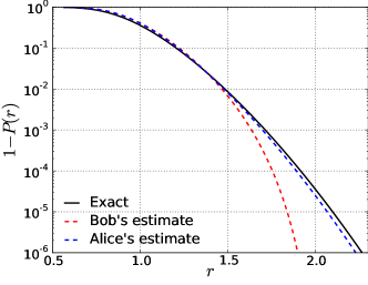
Figure 1: Comparison of the exact and estimated probability of the radius of the largest of 10 disks being greater than $r$. Bob’s estimate, based on the extreme value theory, largely underestimate the probability of observing disks with large radii, while Alice’s estimate, based on treating area as the primary random variable, and transforming back the results to get probability of radii, works much better.

A great deal of insight about convergence issues in extreme value statistics can be gained by analyzing this example. Let $P(A<a),\ P(R<r)$ be the probabilities that the area, radius of a disk are lesser than $a$, $r$, respectively. Clearly, $P(A<a)=1-e^{-a}$ and $P(R<r)=1-e^{-\pi r^{2}}$. It is also clear that the tail of radius distribution, $P(R<r)$, decays faster than exponentially for large $r$, thus any extreme value distribution, $G_{\gamma}(\cdot)$, will not be able to model it accurately. On the other hand, the tail of the area distribution, $P(A<a)$, decays exponentially, and can be modeled accurately by $G_{0}(\cdot)$. Thus, there is an inherent advantage to working with $A$ as the random variable being fit to extreme value distributions, even though $A$ and $R$ are simply related by $A=\pi R^{2}$. After a fit has been obtained for $A$, the probability for $R$ can be obtained easily by transforming back via $P(R<r)=P(A<\pi r^{2})$. Figure 1 shows a comparison of Bob’s and Alice’s estimates and the exact result. Since there were 100 boxes, the empirical data was available at a probability level of $1-P=10^{-2}$. Up to this level both estimates agree reasonably with the exact result. However, at $r=1.91$, the exact result is $1-P(r)=10^{-4}$, Bob’s estimate is $1-P_{B}(r)=4.5\times 10^{-7}$, and Alice’s estimate is $1-P_{A}(r)=7.3\times 10^{-5}$. Thus, Alice’s estimate is off by about 25%, while Bob’s is off by more than two orders of magnitude. Formally, one can show that $W(n)\sim 1/2n$, $\sim 1/\log n$, for Alice’s and Bob’s estimates, respectively.

The insight gained from the above example can be formalized. The idea is that it can be advantageous to work with a suitably transformed variable, instead of the raw data itself. The extreme value estimate for the raw data, $P(X_{n}<x)\approx G_{\gamma_{x}}((x-b_{nx})/a_{nx})$ is susceptible to all the convergence issues discussed previously.

Claim: There exists a monotonic $n$-independent transformation $\tilde{Y}=\hat{T}(\tilde{X})$ and constant $\gamma$ such that the extreme value approximation is exact, i.e. $P(X_{n}<x)=P(Y_{n}<\hat{T}(x))=G_{\gamma}((\hat{T}(x)-b_{ny})/a_{ny})$ for suitable $n$-dependent constants $b_{ny},\ a_{ny}$, where $Y_{n}=\mathrm{max}(\tilde{Y}_{1},\ldots,\tilde{Y}_{n})$.

Proof: $\hat{T}(x)=G_{0}^{-1}(F(x))$, $\gamma=0$, $a_{ny}=1$, $b_{ny}=\log n$ are suitable, as can be checked by direct substitution. However, this choice is not unique.  $\blacksquare$

Thus, working with a suitably transformed variable $\tilde{Y}=\hat{T}(\tilde{X})$ completely suppresses the systematic errors of the extreme value approximation in the sense of Eqs. 1, 2. However, there is a slight problem with this scheme: it demands that to construct $\hat{T}(\cdot)$ we know $F(\cdot)$, which if we knew, we could calculate $F(\cdot)^{n}$ exactly without this elaborate scheme anyway! This problem is made tractable by the following results.

Claim: Let $F(\cdot)$ have unbounded support (the case of bounded support is similar). Let $F(x)\sim 1-\sum_{i=0}^{\infty}f_{i}(x)$ be an asymptotic expansion for large $x$, where the gauge functions $f_{i}(\cdot)$ are monotonic. Then the variable $\tilde{Y}=T(\tilde{X})=-\log f_{0}(\tilde{X})$ is asymptotically exponentially distributed, and for the Edgeworth expansion corresponding to the variable $\tilde{Y}$ (Eq. 1) the rate of convergence, and the quality of the upper tail are characterized by

$$W(n)\sim 1/2n,$$ (4)

$$(1-P(Y_{n}<y+\log n))/(1-G_{0}(x))\to 1.$$ (5)

Proof: Since $f_{0}(\cdot)$ is monotonic, $T^{-1}(x)=f_{0}^{-1}(e^{-x})$. Now, $P(\tilde{Y}<y)=P(\tilde{X}<T^{-1}(y))=F(f_{0}^{-1}(e^{-y}))\sim 1-e^{-y}.$ Thus, the distribution of $\tilde{Y}$ is asymptotically exponential. Eqs. 4, 5 hold due to properties of the standard exponential distribution (see supplemental section I.7 for detailed proof).  $\blacksquare$ Thus, instead of knowing $F(\cdot)$ it is sufficient to estimate $f_{0}(\cdot)$. Since $P(Y_{n}<y)=P(X_{n}<T^{-1}(y))$, we get the following convergence assurances based on Eqs. 4, 5

$$\lim_{n\to\infty}\frac{F(T^{-1}(x+\log n))^{n}-G_{0}(x)}{1/2n}=G^{\prime}_{0}(x)\hat{H}_{0}[G_{0}(x)],$$ (6)

$$({1-F(T^{-1}(x+\log n))^{n}})/({1-G_{0}(x)})\to 1,$$ (7)

where $\hat{H}_{0}[G_{0}(x)]=e^{-x}+x-1$ (supplemental section I.7). We have taken the norming constants $a_{ny},\ b_{ny}=1,\ \log n$, as these are the theoretical asymptotic values for the exponential distribution. In practice they must be treated as free parameters to be fit.

The proposed method, which we call the T-method (‘T’ for transformation), is now clear. Let us say that we can parameterize the transformation $T(x)=-\log f_{0}(x)$ by a parameter $\beta$, then we have a parameter vector $\theta=(\beta,a_{n},b_{n})$, and a model $G_{0}((T(\mathbf{X}|\beta)-b_{n})/a_{n})$. Given data vector $\mathbf{X}=(X_{n_{1}},X_{n_{2}},\ldots,X_{n_{m}})$, the parameter vector $\theta$ can be estimated via the maximum likelihood method by maximizing the following likelihood function

$$\mathcal{L}(\theta|\mathbf{X})=\sum_{i=1}^{m}\big{(}\log G^{\prime}_{0}((T(\mathbf{X}_{i})-b_{n})/a_{n})+\log T^{\prime}(\mathbf{X}_{i})/a_{n}\big{)}.$$ (8)

As a final step, the transformation $T(\cdot)$ needs to be parameterized by the parameter $\beta$ in a principled way. As mentioned previously, we restrict our discussion to distributions in the domain of $G_{0}(\cdot)$, and a transformation of the form discussed next will be useful only if for the raw data we get $\gamma$ close to 0. The required transformation can be worked out easily for several common distributions with $F\in D(G_{0})$. For example (supplemental section I.5), for the normal distribution we get $f_{0}(x)=e^{-x^{2}/2}/\sqrt{2\pi}x$, $T(x)=-\log f_{0}(x)\sim x^{2}$ (strictly speaking $T(x)\sim x^{2}/2+\log(x/\sqrt{2\pi})$, however multiples can be absorbed into $a_{n}$, constants into $b_{n}$, and we ignore the asymptotically smaller $\log x$), for Rayleigh type distributions $F(x)=1-e^{-x^{\alpha}}$, $T(x)=x^{\alpha}$, for lognormal distribution $T(x)\sim(\log x)^{2}$ etc. The heuristic is that if a semilog plot of $1-\hat{C}_{n}(x)$, where $\hat{C}_{n}(x)$ is the empirical cdf of the data, is a straight line, then the underlying distribution $1-F(x)$ is exponential, and no correction is needed. If the plot curves downwards, then $1-F(x)$ decays super-exponentially, and $T(x)=x^{\beta}$ with $\beta>1$. If the semilog plot curves upwards, while a loglog plot curves downwards, then the decay is super-polynomial, but sub-exponential, thus $T(x)$ is of the form $x^{\beta}$ with $0<\beta<1$ or of the form $\log(x)^{\beta}$. If the loglog plot is roughly straight, then it is likely that $F\notin D(G_{0})$, and either a correction is not needed or it is more subtle, and will be discussed in a later paper. Once a form is chosen, the parameter set $\beta,\ a_{n},\ b_{n}$ can be obtained by using MLE estimator suggested in Eq. 8 or another estimator in the usual manner. Note that $\gamma=0$ is held fixed, so there are still only three free parameters in the model. The classical extreme value fit is a special case of the T-method obtained when $T(\cdot)$ is taken to be the identity, i.e. $T(x)=x$.

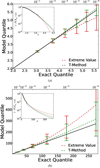
Figure 2: Comparison of the classical extreme value approximation with the suggested transformation based method for data taken from (a) the normal distribution, and (b) the lognormal distribution. The main graph shows the traditional QQ plot with the upper $x$-axis showing the exceedance, $1-P(X_{n_{i}})$ corresponding to the quantile on the main $x$-axis. The solid black line is a guide to the eye and shows the ideal result. The dashed lines show the model quantiles averaged over 1000 monte carlo runs; while the errorbars show the 2-standard deviation range. In each monte carlo run the model fit to a sample of size $m=1000$, and the fit is extrapolated to a probability level of $1-P(X_{n_{i}}<x)=10^{-6}$. The insets show the upper tail of the estimation, $1-P(X_{n_{i}}<x)$, on a semilog plot for a typical monte carlo run; the empirical data is shown in the black dots. It is clear that the transformation based method yields better predictions and less variance even when extrapolated well beyond the range of the available data.

We test the proposed method on data generated from normal and lognormal distributions. For the case of the normal (lognormal) distribution, we generate a random sample $\mathbf{X}=(X_{n_{1}},\ldots,X_{n_{m}})$, where $m=1000$. Each $X_{n_{i}}=\mathrm{max}(\tilde{X}_{1},\ldots,\tilde{X}_{n})$ where $n=100$, and $\tilde{X}_{i}$ are iid random variables drawn from the normal (lognormal) distribution. We estimate the parameter vector $\mathbf{\theta}=(\beta,a_{n},b_{n})$ by using MLE (Eq. 8) with $T(x|\beta)=x^{\beta}$ for the normal case, and $T(x|\beta)=(\log x)^{\beta}$ for the lognormal case. Figure 2 shows a favorable comparison of the results obtained by the T-method with the classical extreme value approximation. We have also tested the method on other distributions, including Rayleigh type distributions, and the Leath-Duxbury distribution encountered in statistics of fracture duxbury1987 . It is clear that the suggested method out-performs the classical extreme value approximation with the same number of parameters. Finally, we tested the method on the exponential distribution, where the convergence to $G_{0}(\cdot)$ is rapid, and a correction is not needed per se. We found that the T-method increases the mean accuracy of predictions slightly, while reducing the spread in the predictions significantly (supplemental section I.8).

In summary, we have suggested a simple method, which we call the T-method, to alleviate the problem of slow convergence of classical extreme value approximations. The method works by estimating simple nonlinear transformation that defines a new random variable that has better convergence properties in the extreme value sense. Some previous authors have studied rates of convergence in nonlinear scaling in extreme value statistics (see Refs. pantcheva1985 ; barakat2010 ). Their results are rather remarkable, however, their focus has been on studying $d_{n}$ or $W(n)$ for specific transformations (power transformation, for example) rather than constructing numerical methods of wide applicability. In this sense the proposed T-method is complementary to their results. The T-method was applied succesfully to distributions in the domain of attraction of the Gumbel (type I) distribution. We hope that application of our method will lead to more reliable estimates of probabilities of extremes in a large number of applications.

I Supplemental Material

I.1 Domain of Attraction

Let $F(\cdot)$ be cumulative distribution function (cdf). A theorem due to Gnedenko (and modified by others to get various characterizations) is stated below; see Refs. resnick1987extreme ; kotz2000 ; coles2001 for proofs.

Theorem I.1

If there exists a sequence of normalizing constants $a_{n}>0$ and $b_{n}\in\Re$, such that

$$F(a_{n}x+b_{n})^{n}\to G_{\gamma}(x),1+\gamma x>0,$$ (9)

weakly as $n\to\infty$, then $G_{\gamma}(x)$ is of the form

$$G_{\gamma}(x)=\exp\{-(1+\gamma x)^{-1/\gamma}\},\quad\gamma\in\Re.$$ (10)

In such a case we say that $F(\cdot)$ is in the domain of attraction of $G_{\gamma}(\cdot)$, or $F\in D(G_{\gamma})$. A characterization of the domain of attraction is as follows.

Theorem I.2

(See Ref. haan1996 for details) Let

$$j\equiv\left(\frac{1}{-\log F}\right)^{-1},$$ (11)

where the $(\cdot)^{-1}$ denotes inverse, i.e., under suitable continuity conditions $j(x)\equiv F^{-1}(e^{-1/x})$. Then Eq. 9 holds iff

$$\lim_{t\to\infty}\frac{j(tx)-j(t)}{tj^{\prime}(t)}=\frac{x^{\gamma}-1}{\gamma}.$$ (12)

A sufficient condition for Eq. 9 to hold is

$$\lim_{t\to\infty}\frac{j^{\prime}(tx)}{j^{\prime}(t)}=x^{\gamma-1}$$ (13)

I.2 Norming Constants

Theorem I.3

(See Ref. haan1996 for details) The following constants are asymptotically optimal norming constants in Eq. 9

$$a_{n}=nj^{\prime}(n),\quad b_{n}=j(n).$$ (14)

I.3 Rates of Uniform Convergence and Edgeworth Expansions

Let $F\in D(G_{\gamma})$, and

$$d_{n} =\sup_{n}|F(a_{n}x+b_{n})^{n}-G_{\gamma}(x)|,$$ (15)

$$x_{0} =\sup\left\{x:F(x)<1\right\},$$ (16)

$$h(x) =-\log F(x)-\left\{\frac{-F(x)F^{\prime\prime}(x)\log F(x)}{(F^{\prime}(x))^{2}}+1\right\}.$$ (17)

Let $g(x)$ be such that

$$|h(x)|\leq g(x)\downarrow 0\ \mathrm{as}\ x\to x_{0}.$$ (18)

Theorem I.4

(See Ref. resnick1987extreme section 2.4.2 for details) Let If $F\in D(G_{0})$ then $d_{n}\leq O(g(b_{n})).$

Theorem I.5

(See Ref. haan1996 for details) Let $F\in D(G_{\gamma})$, then

$$\lim_{n\to\infty}\frac{F(a_{n}x+b_{n})^{n}-G_{\gamma}(x)}{W(n)}=G^{\prime}_{\gamma}(x)\hat{H}_{\gamma}[G_{\gamma}(x)],$$ (19)

uniformly in $x$, where $\hat{H}_{\gamma}(G_{\gamma}(x))=H_{\gamma}(-\log(-\log G_{\gamma}(x)))$ and

$$H_{\gamma}(x)=\left\{\begin{array}[]{ll}\int_{0}^{x}e^{\gamma u}\int_{0}^{u}e^{\rho s}dsdu&\mathrm{for}\ \gamma\geq 0\\ -\int_{x}^{\infty}e^{\gamma u}\int_{0}^{u}e^{\rho s}dsdu&\mathrm{for}\ \gamma<0.\end{array}\right.,$$ (20)

where $\rho$ is such that for $v(t)\equiv j(e^{t})$, and $A(e^{t})\equiv v^{\prime\prime}(t)/v^{\prime}(t)-\gamma$,

$$\lim_{t\to\infty}\frac{A(tx)}{A(t)}=x^{\rho}\ \mathrm{for}\ x>0.$$ (21)

The function $W(n)$ is given by

$$W(n)=nj^{\prime\prime}(n)/j^{\prime}(n)-\gamma+1.$$ (22)

I.4 Examples

I.4.1 Exponential Distribution

For the standard exponential distribution, $F(x)=1-e^{-x}$, $F^{-1}(x)=-\log(1-x)$. We get

$$j(x)=F^{-1}(e^{-1/x})\sim\log x+\frac{1}{2x}+O(1/x^{2}).$$ (23)

Thus,

$$a_{n}=nj^{\prime}(n)\sim 1,\quad b_{n}=j(n)\sim\log n.$$ (24)

Further

$$h(x) =-\log F(x)-\left\{\frac{-F(x)F^{\prime\prime}(x)\log F(x)}{(F^{\prime}(x))^{2}}+1\right\}$$ (25)

$$=-1-e^{x}\log(1-e^{-x})$$ (26)

$$=\frac{e^{-x}}{2}+\frac{e^{-2x}}{3}+\frac{e^{-3x}}{4}+\ldots$$ (27)

$$<e^{-x}.$$ (28)

Thus we get $g(x)=e^{-x}$ and $g(b_{n})=1/n$, so that

$$d_{n}=\sup_{n}|F(a_{n}x+b_{n})^{n}-G_{\gamma}(x)|\leq O(1/n)$$ (29)

Grinding through the calculations further gives $A(t)\sim 1/(2t-1)$, thus, $\rho=-1$. Thus,

$$H_{\gamma}(x)=\int_{0}^{x}e^{\gamma u}\int_{0}^{u}e^{\rho s}dsdu=e^{-x}+x-1$$ (30)

which yields

$$\hat{H}_{\gamma}(x)=e^{-x}+x-1.$$ (31)

The function $W(n)$ is

$$W(n)=nj^{\prime\prime}(n)/j^{\prime}(n)-\gamma+1\sim 1/2n.$$ (32)

Thus, the Edgeworth expansion becomes

$$\lim_{n\to\infty}\frac{F(a_{n}x+b_{n})^{n}-G_{0}(x)}{1/2n}=G^{\prime}_{0}(x)(e^{-x}+x-1)$$ (33)

I.4.2 Normal Distribution

$$F(x)=\frac{1}{\sqrt{2\pi}}\int_{-\infty}^{x}e^{-t^{2}/2}dt\sim 1-\frac{e^{-x^{2}/2}}{x\sqrt{2\pi}}\left(1-\frac{1}{x^{2}}\right)$$ (34)

Since $F(j(x))=e^{-1/x}$, so for large $x$, $j(x)$ must be suitably large. However, $j(x)$ might not grow rapidly enough with $x$, so we keep a higher order term for $j(x)$ in the following expansion

$$F(j(x)) =e^{-1/x}$$ (35)

$$1-\frac{e^{-j(x)^{2}/2}}{j(x)\sqrt{2\pi}}\left(1-\frac{1}{j(x)^{2}}\right) \approx 1-\frac{1}{x}$$ (36)

$$j^{2}/2+\log j-\log(1-\frac{1}{j^{2}})\approx\log(x/\sqrt{2\pi})$$ (37)

$$j^{2}/2+\log j+1/j^{2}\approx\log(x/\sqrt{2\pi})$$ (38)

Ignoring the $1/j^{2}$ and solving gives

$$j(x)\sim\sqrt{2\log\tilde{x}-\log(2\log\tilde{x})},$$ (39)

where $\tilde{x}=x/\sqrt{2\pi}$. Grinding through the details, we get

$$b(n)\sim\sqrt{2\log\tilde{n}-\log(2\log\tilde{n})},$$ (40)

$$a(n)\sim 1/b(n),\ W(n)\sim-1/2\log(n).$$ (41)

Further calculations show that $A(t)\sim-1/2\log t$, giving $\rho=0$ and

$$H_{\gamma}(x)=\int_{0}^{x}e^{\gamma u}\int_{0}^{u}e^{\rho s}dsdu=x^{2}/2$$ (42)

which yields

$$\hat{H}_{\gamma}(x)=x^{2}/2.$$ (43)

Thus, the Edgeworth expansion becomes

$$\lim_{n\to\infty}\frac{F(a_{n}x+b_{n})^{n}-G_{0}(x)}{-1/2\log n}=G^{\prime}_{0}(x)\frac{x^{2}}{2}$$ (44)

I.4.3 LogNormal Distribution

$$F(x) =\frac{1}{\sqrt{2\pi}}\int_{-\infty}^{\log x}e^{-t^{2}/2}dt$$ (45)

$$\sim 1-\frac{e^{-(\log x)^{2}/2}}{\log x\sqrt{2\pi}}\left(1-\frac{1}{(\log x)^{2}}\right).$$ (46)

The analysis proceeds in a manner analogous to the last section. The first order results are

$$a(n)\sim e^{D(n)}/D(n),\ b(n)\sim e^{D(n)},\ W(n)\sim-1/D(n),$$ (47)

where $D(n)=(2\log(n/\sqrt{2\pi}))^{1/2}$.

I.4.4 Rayleigh Distribution

$$F(x)=1-e^{-x^{\alpha}},\quad F^{-1}(x)=(-\log(1-x))^{1/\alpha}$$ (48)

Auxiliary function $j$

$$j(x) =F^{-1}(e^{-1/x})$$ (49)

$$\sim(\log x)^{1/\alpha}\left(1+\frac{1}{2\alpha x\log x}\right)$$ (50)

Thus

$$b(n) \sim(\log n)^{1/\alpha}$$ (51)

$$a(n) \sim\frac{(\log n)^{1/\alpha-1}}{\alpha}$$ (52)

$$W(n) \sim\frac{1-\alpha}{a\log n}+\frac{1}{2n}$$ (53)

I.4.5 Gamma Distribution

$$F(x) =\frac{1}{\Gamma(a)}\int_{0}^{x}t^{a-1}e^{-t}dt$$ (54)

$$\sim 1-\frac{x^{a-1}e^{-x}}{\Gamma(a)}\left(1+\frac{a-1}{x}+\frac{(a-1)(a-2)}{x^{2}}+\ldots\right)$$ (55)

Thus

$$j(x) \sim\log(x/\Gamma(a))+(a-1)\log(\log(x/\Gamma(a)))$$ (56)

$$b(n) \sim\log(n/\Gamma(a))+(a-1)\log(\log(x/\Gamma(a)))$$ (57)

$$a(n) \sim 1+(a-1)/\log(x/\Gamma(a))$$ (58)

$$W(n) \sim-\frac{a-1}{(a-1+\log(x/\Gamma(a)))\log(x/\Gamma(a))}$$ (59)

I.5 Transformations

This section has the calculation for the asymptotic terms in the mapping $G^{-1}_{0}(F(x))$ for some $F(x)$.

I.5.1 Normal

The normal cdf is,

$$F(x)=\frac{1}{\sqrt{2\pi}}\int_{-\infty}^{x}e^{-t^{2}/2}dt\sim 1-\frac{e^{-x^{2}/2}}{x\sqrt{2\pi}}\left(1-\frac{1}{x^{2}}\right).$$ (60)

while the inverse of $G_{0}(\cdot)$ is

$$G^{-1}_{0}(x) =-\log(-\log(x))$$ (61)

$$G^{-1}_{0}(1-x) \sim-\log(x)-\frac{x}{2}-\frac{5x^{2}}{24}-\ldots.$$ (62)

Thus, the transformation becomes

$$G^{-1}_{0}(F(x))\sim\frac{x^{2}}{2}+\log\left(x\sqrt{2\pi}\right)+\mathcal{O}(1/x^{2})$$ (63)

I.5.2 Lognormal

The lognormal cdf is

$$F(x)\frac{1}{\sqrt{2\pi}}\int_{-\infty}^{\log x}e^{-t^{2}/2}dt.$$ (64)

Thus, the transformation becomes

$$G^{-1}_{0}(F(x))\sim\frac{(\log x)^{2}}{2}+\log\left(\log x\sqrt{2\pi}\right)+\mathcal{O}(1/\log x^{2})$$ (65)

I.5.3 Rayleigh

The Rayleigh cdf is

$$F(x)=1-e^{-x^{\alpha}}$$ (66)

Thus the transformation becomes

$$G^{-1}_{0}(F(x))\sim x^{\alpha}-\frac{e^{-x^{\alpha}}}{2}+\ldots$$ (67)

I.5.4 Gamma

The Gamma cdf is

$$F(x) =\frac{1}{\Gamma(a)}\int_{0}^{x}t^{a-1}e^{-t}dt$$ (68)

$$\sim 1-\frac{x^{a-1}e^{-x}}{\Gamma(a)}\left(1+\frac{a-1}{x}+\frac{(a-1)(a-2)}{x^{2}}+\ldots\right)$$ (69)

Thus, the transformation becomes

$$G^{-1}_{0}(F(x))\sim x+(1-a)\log x+\log\Gamma(a)$$ (70)

I.6 Tail Convergence

I.6.1 Exponential Distribution

The exponential cdf and norming constants are

$$F(x)=1-e^{-x},\ a_{n}=1,\ b_{n}=\log n.$$ (71)

Thus,

$$L(x) =\frac{1-F(a_{n}x+b_{n})^{n}}{1-G_{0}(x)}$$ (72)

$$=\frac{1-(1-e^{-x}/n)^{n}}{1-e^{-e^{-x}}}$$ (73)

$$=\frac{e^{-x}+o(e^{-x})}{e^{-x}+o(e^{-x})}\to 1,$$ (74)

where $o()$ is the ‘small-$o$’ notation. Thus, the extreme value approximation for the exponential distribution is good in the upper tail of the distribution.

I.6.2 Normal Distribution

The normal cdf and norming constants are

$$F(x)=\frac{1}{\sqrt{2\pi}}\int_{-\infty}^{x}e^{-t^{2}/2}dt\sim 1-\frac{e^{-x^{2}/2}}{x\sqrt{2\pi}}\left(1-\frac{1}{x^{2}}\right),$$ (75)

$$b(n)\sim\sqrt{2\log\tilde{n}-\log(2\log\tilde{n})},\ a(n)\sim 1/b(n),\ \tilde{n}=n/\sqrt{2\pi}.$$ (76)

Thus, it is easy to see that

$$L(x) =\frac{1-F(a_{n}x+b_{n})^{n}}{1-G_{0}(x)}\to 0$$ (77)

Thus, the extreme value approximation for the normal distribution is bad in the upper tail.

I.7 Proofs

Claim: Let $F(\cdot)$ have unbounded support (the case of bounded support is similar). Let $F(x)\sim 1-\sum_{i=0}^{\infty}f_{i}(x)$ be an asymptotic expansion for large $x$, where the gauge functions $f_{i}(\cdot)$ are monotonic. Then the variable $Y=T(X)=-\log f_{0}(x)$ is asymptotically exponentially distributed, i.e.,

$$P(Y<y)\sim 1-e^{-y},$$ (78)

and

$$\lim_{n\to\infty}\frac{P(Y_{n}<y+\log n)-G_{0}(y)}{W(n)}=G^{\prime}_{0}(y)\hat{H}_{0}[G_{0}(y)],$$ (79)

where $W(n)\sim 1/2n$, and

$$(1-P(Y_{n}<y+\log n))/(1-G_{0}(x))\to 1.$$ (80)

Proof: Since $f_{0}(\cdot)$ is monotonic, $T^{-1}(x)=f_{0}^{-1}(e^{-x})$. Now,

$$K(y)\equiv P(Y<y) =P(X<T^{-1}(y))$$ (81)

$$=F(f_{0}^{-1}(e^{-y}))$$ (82)

$$\sim 1-e^{-y}.$$ (83)

Thus, the distribution of $Y$ is asymptotically exponential. Consider the auxiliary function $j(n)$. By definition

$$K(j(n))=e^{-1/n},$$ (84)

Thus, $j(n)\to\infty$ as $n\to\infty$, since it is easy to check that $K(y)$ is monotonic and $\lim_{y\to\infty}K(y)=1$. Thus, for large $n$ we can use the asymptotic expansion $K(j(n))\sim 1-e^{-j}+o(e^{-j})$. The monotonity of the gauge functions $f_{i}(\cdot)$ ensure that there are no oscillatory terms in this asymptotic expansion, and thus it can be differentiated term by term. Thus, we have

$$1-e^{-j(n)}+o(e^{-j(n)})\sim e^{-1/n}.$$ (85)

The above has the solution

$$j(n)\sim-\log(1-e^{-1/n})+o(1/n),$$ (86)

as can be verified by direction substitution. Thus, for the Edgeworth expansion (theorem I.5), we get

$$W(n)=nj^{\prime\prime}(n)/j^{\prime}(n)-\gamma+1=nj^{\prime\prime}(n)/j^{\prime}(n)+1\sim 1/2n.$$ (87)

Further following theorem I.5, we get $A(t)\sim 1/2t$, thus giving $\rho=-1$. Since $\gamma=0$, we get $\hat{H}_{0}[G_{0}(x)]=e^{-x}+x+1$ from theorem I.5. The Edgeworth expansion is thus established. Finally, for the tail approximation

$$L(y) =\frac{1-P(Y_{n}<y+\log n)}{1-G_{0}(y)}$$ (88)

$$=\frac{1-K(y+\log n)^{n}}{1-G_{0}(y)}$$ (89)

$$=\frac{1-(1-e^{-y}/n+o(e^{-y}/n))^{n}}{1-e^{-e^{-y}}}$$ (90)

$$=\frac{e^{-y}+o(e^{-y})}{e^{-y}+o(e^{-y})}\to 1,$$ (91)

and the proof is complete.  $\blacksquare$

I.8 Fits to Exponential Data

Here we apply the T-method to the standard exponential distribution, $F(z)=1-e^{-z}$. Since the convergence of the exponential distribution to the extreme value form $G_{0}(\cdot)$ is rapid in the bulk as well as in the tail, the application of the T-method is not necessary to get a good fit to the data, or a good result from the extrapolation of the fit. However, we apply the method to test if its application in such a case result in predictions that are any worse (or better) than the standard extreme value statistics. In particular, we consider the distribution of the variable $X$ = $\mathrm{max}(Z_{1},\ldots,Z_{m})$, where $Z_{i}$ are exponential iid random variables, $P(Z_{i}<z)=F(z)=1-e^{-z}$. We take $m=100$, and take a sample $\mathbf{X}=(X_{1},\ldots,X_{n})$ of size $n=1000$. The classical extreme value model is parameterized by the parameter vector $\theta_{c}=(\gamma,a_{n},b_{n})$, and leads to the following log-likelihood function

$$\mathcal{L}_{c}(\theta_{c}|\mathbf{X})={\Sigma}_{i}\big{(}\log G^{\prime}_{\gamma}((X_{i}-b_{n})/a_{n})+\log(\gamma/a_{n})\big{)}.$$ (92)

While, the T-method with the transformation $Y=T(X|\beta)=X^{\beta}$ is parameterized by the parameter vector $\theta_{t}=(\beta,a_{n},b_{n})$ and leads to the following log-likelihood function

$$\mathcal{L}_{t}(\theta_{t}|\mathbf{X})={\Sigma}_{i}\big{(}\log G^{\prime}_{0}((T(X_{i}|\beta)-b_{n})/a_{n})\\ +\log T^{\prime}(X_{i}|\beta)-\log a_{n}\big{)}.$$ (93)

We do monte carlo simulations by generating 1000 samples $\mathbf{X}$ and fitting the models. Figure 3 shows the mean and the 2-standard deviation bounds for the QQ plots of the fits. It is clear that the mean prediction from T-method is slightly better than the classical extreme value fit, while the T-method results in smaller variance in the predictions.

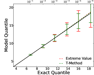
Figure 3: Comparison of the classical extreme value approximation with the suggested transformation based method for data taken from the standard exponential distribution. The solid black line is a guide to the eye and shows the ideal result. The dashed lines show the model quantiles averaged over 1000 monte carlo runs; while the errorbars show the 2-standard deviation range. In each monte carlo run the model fit to a sample of size 1000, and the fit is extrapolated to a probability level of $1-P(X_{n}<x)=10^{-6}$. The insets show the upper tail of the estimation, $1-P(X_{n}<x)$, on a semilog plot for a typical monte carlo run; the empirical data is shown in the black dots. It is clear that the transformation based method yields better predictions and less variance even when extrapolated well beyond the range of the available data.

References

(1)In a broad sense the term ‘universal’ refers to any behavior
that is largely independent of details, and is shared across a broad class.
For example, the mean of iid random variables has a Gaussian distribution
under very general conditions. This behavior is largely independent of the
details of the distribution of the iid variables, and thus is universal. In
similar spirit, the generalized extreme value distribution is a universal
description of large statistical fluctuations.
(2)F. M. Longin, J. Of Business 69 (July 1996)
(3)J. P. Broussard and G. G. Booth, European Journal of Operational Research 104, 393 (1998)
(4)R. W. Katz, M. B. Parlange, and P. Naveau, Advances in Water Resources 25, 1287 (2002)
(5)J.-T. Shiau, S. Feng, and S. Nadarajah, Hydrological Processes 21, 2157 (2007)
(6)M. N. Khaliq, T. B. M. J. Ouarda, J.-C. Ondo, P. Gachon, and B. Bobee, Journal of Hydrology 329, 534 (2006)
(7)W. Weibull, A statistical theory of the strength of materials (Stockholm, 1939)
(8)D. G. Harlow and S. L. Phoenix, Journal of Composite Materials 12, 195 (1978)
(9)P. M. Duxbury, P. L. Leath, and P. D. Beale, Phys. Rev. B 36, 367 (Jul 1987)
(10)C. Manzato, A. Shekhawat, P. K. V. V. Nukala, M. J. Alava, J. P. Sethna, and S. Zapperi, Phys. Rev. Lett. 108, 065504 (Feb 2012)
(11)T. A. Buishand, Statistica Neerlandica 43, 1 (1989)
(12)R. L. Smith, Statistical Science 4, 367 (11 1989)
(13)P. Embrechts, S. I. Resnick, and G. Samorodnitsky, North American Actuarial Journal 3, 30 (1999)
(14)A. J. McNeil and R. Frey, Journal of Empirical Finance 7, 271 (2000)
(15)J. Beirlant and J. L. Teugels, Insurance: Mathematics and Economics 11, 17 (1992)
(16)R. Holger and T. Nader, Scandinavian Actuarial Journal 1997, 70 (1997)
(17)S. J. Roberts, Science, Measurement and Technology, IEE Proceedings - 147, 363 (Nov 2000)
(18)P. B. Gnedenko, Annals of Mathematics 44, 423 (1943)
(19)L. de Haan, On regular variation and its application to the weak
convergence of sample extremes, Mathematical Center Tracts 32 (Mathematisch Centrum, Amsterdam,
Holland, 1970)
(20)S. I. Resnick, Extreme values, regular variation and point
processes (Springer Verlag, New York, 2007)
(21)L. de Haan and S. I. Resnick, The Annals of Probability 24, 97 (1996)
(22)S. Kotz and S. Nadarajah, Extreme value distributions (World Scientific, 2000)
(23)M. I. Gomes, Annals of the Institute of Statistical Mathematics 36, 71 (1984)
(24)J. P. Cohen, Advances in Applied Probability 14, pp. 833 (1982), ISSN 00018678
(25)G. Györgyi, N. R. Moloney, K. Ozogány, Z. Rácz, and M. Droz, Phys. Rev. E 81, 041135 (Apr 2010)
(26)C. W. Anderson, Journal of the Royal Statistical Society. Series B
(Methodological) 40, 197 (1978)
(27)C. Anderson, in Statistical Extremes and Applications, NATO ASI Series, Vol. 131, edited by J. Oliveira (Springer
Netherlands, 1984) pp. 325–340
(28)A function is said to the regularly varying with
index at if . It is called slowly varying if .
(29)E. Pantcheva, in Stability Problems for Stochastic Models, Lecture Notes in Mathematics, Vol. 1155, edited by V. V. Kalashnikov and V. M. Zolotarev (Springer Berlin Heidelberg, 1985) pp. 284–309
(30)H. M. Barakat, E. M. Nigm., and M. E. El-Adll, Statistical Papers 51, 149 (2010)
(31)S. Coles, J. Bawa, L. Trenner, and P. Dorazio, An introduction to statistical modeling of extreme
values, Vol. 208 (Springer, 2001)