3D-HST Emission Line Galaxies at $z\sim 2$: Discrepancies in the Optical/UV Star Formation Rates

Abstract

We use Hubble Space Telescope near-IR grism spectroscopy to examine the H$\beta$ line strengths of 260 star-forming galaxies in the redshift range $1.90<z<2.35$. We show that at these epochs, the H$\beta$ star formation rate (SFR) is a factor of $\sim$ 1.8 higher than what would be expected from the systems’ rest-frame UV flux density, suggesting a shift in the standard conversion between these quantities and star formation rate. We demonstrate that at least part of this shift can be attributed to metallicity, as H$\beta$ is more greatly enhanced in systems with lower oxygen abundance. This offset must be considered when measuring the star formation rate history of the universe. We also show that the relation between stellar and nebular extinction in our $z\sim 2$ sample is consistent with that observed in the local universe.

1. Introduction

Star formation and the build-up of stellar mass are key astrophysical parameters for our understanding of galaxy evolution and formation. By quantifying the amount of star formation over a given time scale and co-moving volume, we can constrain models of galaxy formation, chemical enrichment (both interior and exterior to galaxies), and the ionization history of the intergalactic medium (e.g., Tinsley, 1980; Madau et al., 1996). However, the process of converting observables, such as a galaxy’s Balmer emission or UV flux density, into actual star formation rates (SFRs) is fraught with difficulty, since virtually all common SFR indicators are indirect and sensitive only to the presence of high-mass, short-lived stars. Assumptions concerning the shape of the initial mass function (IMF), the star formation history of the population, and the metal abundance of the stars all play a role in translating measurable quantities into physical star formation rates.

Kennicutt (1998) and Kennicutt & Evans (2012) have reviewed the commonly used SFR indicators, their calibration, and their limitations. Two of the most useful of these are a galaxy’s UV luminosity density and the energy emitted in its Balmer lines. The former is produced by stars with $M\gtrsim 5M_{\odot}$, and therefore records star formation over the last $\sim 100$ Myr. The method is extremely sensitive to dust, as just a few tenths of differential reddening can lead to magnitudes of extinction, and its calibration depends on a number of assumptions, including that of the population’s IMF, metallicity, and star formation rate history. Nevertheless, it is the technique most commonly used for SFR measurements in the high-redshift universe. In contrast, emission lines such as H$\alpha$ and H$\beta$ are the result of the ionizing photons produced by stars with $M\gtrsim 15M_{\odot}$, and thus probe only the most recent episode of star formation, i.e., stars with ages of $t<10$ Myr. Like the UV, Balmer emission also depends on the population’s IMF, metallicity, and extinction, but the reaction of these lines to changes in the stellar population parameters is different. As a result a comparison of the two indicators can provide insights into both the stellar population and extinction, even in the absence of additional information (e.g., Lee et al., 2009; Meurer et al., 2009).

In this paper, we use near-IR spectroscopy with the Hubble Space Telescope (HST) and a wealth of ancillary photometric data to examine the H$\beta$ line strengths and rest-frame UV flux densities of 260 star-forming galaxies in the redshift range $1.90<z<2.35$. In §2, we discuss the data for a combined $\sim$350 arcmin² region of the GOODS-N, GOODS-S, and COSMOS fields, and the reduction techniques needed to measure total H$\beta$ fluxes for galaxies with star formation rates as low as $\sim 2\,M_{\odot}$ yr^-1. In §3, we describe the procedures used to identify a complete, H$\beta$-selected sample of objects at $z\sim 2$, and present our measurements of these galaxies. In §4, we calculate the galaxies’ SFRs using the conversion factors summarized in Kennicutt & Evans (2012) and the local starburst galaxy extinction law found by Calzetti (2001). We show that there is an inconsistency between the two SFRs, and examine the various parameters which might explain the offset. We demonstrate that galactic metallicity is in large part responsible for the SFR discrepancy, and that a Calzetti (2001) law reproduces the ratio of nebular-to-stellar extinction. We conclude by discussing the possible impact of these measurements on other investigations of the high-redshift universe. For this work we adopt a standard $\Lambda$CMD cosmology, with $\Omega_{M}=0.3$, $\Omega_{\Lambda}=0.7$, and $H_{0}=70$ km s^-1 Mpc^-1.

2. Data and Reductions

Our study of star formation in the $z\sim 2$ universe is focused on three $\sim 120$ arcmin² patches of sky in the COSMOS (Scoville et al., 2007), GOODS-N, and GOODS-S (Giavalisco et al., 2004) fields. In these regions, there is a wealth of photometry and spectroscopic data available for analysis, including broadband photometry from a host of space missions, broad- and intermediate-band photometry from the ground, and optical and near-IR slitless spectroscopy from HST. Below we describe the data used in our analysis.

2.1. Optical/Near-IR Imaging

To perform our analysis, we took advantage of the Skelton et al. (2014) photometric catalogs produced by the 3D-HST project (Brammer et al., 2012, GO-11600, 12177, and 12328). Skelton et al. (2014) homogeneously combined 147 distinct ground-based and space-based imaging data sets covering the wavelength range $0.3\mu$m to $8.0\mu$m in five well-observed legacy fields, including GOODS-N, GOODS-S, and COSMOS. In their analysis, Skelton et al. (2014) obtained and reduced HST/WFC3 images from both the CANDELS (Grogin et al., 2011) and 3D-HST (Brammer et al., 2012) surveys, and created a source catalog using SExtractor (Bertin & Arnouts, 1996) on co-added F125W+F140W+F160W images. These catalogs, detection segmentation maps, point spread functions (PSFs), and flux enclosed in PSF-matched apertures were then used to measure total flux densities in a wide variety of publicly available imaging datasets. For $z\sim 2$ systems, these data offer unprecedented access to the rest-frame ultraviolet and allow precision measurements of the slope of each object’s rest-frame UV continuum.

2.2. HST Spectroscopy

Our rest-frame optical emission-line measurements come from 3D-HST, a near-IR grism survey with the HST WFC3 camera. The 3D-HST primary observations with the G141 grism consists of $R\sim 130$ slitless spectroscopy between $1.08~{}\mu{\rm m}<\lambda<1.68~{}\mu$m over a 625 arcmin² region of sky, which includes $\sim 80\%$ of the CANDELS footprint; when combined with accompanying direct images through the F140W filter of WFC3, these data provide full coverage of the rest-frame wavelengths 3700-5020 Å for all $1.90<z<2.35$ galaxies with unobscured emission line fluxes brighter than $10^{-17}$ ergs cm^-2 s^-1 (at 1-$\sigma$) which corresponds to unobscured SFRs greater than $\sim 2M_{\odot}$ yr^-1. Included in this wavelength range are the strong emission lines of [O II] $\lambda 3727$, [O III] $\lambda\lambda 4959,5007$, [Ne III] $\lambda\lambda 3869,3960$, and hydrogen (H$\beta$, H$\gamma$ and H$\delta$).

To reduce these data, we began with the pre-processed, calibrated “FLT” files in the HST Data Archive. These are the products of the automated reduction process calwf3, which uses the latest reference files to measure and subtract the bias, correct for non-linearity, flag saturated pixels, subtract the dark image, divide by the flat field, calculate the gain, and apply the flux conversion. This process was identical for both the direct and the grism images, with the exception of the flat fielding step: the grism data were flat fielded at a later stage using the aXe software and a master sky flat.

Each grism observation was accompanied by a shallow ($\sim 200$ s) F140W exposure, which served to define the position of each object’s wavelength zeropoint and trace, and hence facilitate spectral calibrations and extraction. These images were combined using the standard procedures of MultiDrizzle (Fruchter et al., 2009), and then co-added with the deeper CANDELS F125W and F160W frames to match the detection image used in the photometric catalogs of Skelton et al. (2014). These data were processed by SExtractor to produce a master catalog of all objects containing more than five pixels above a 3-$\sigma$ per pixel detection threshold and having a total AB magnitude (Oke & Gunn, 1983) brighter than 26. The positions of these sources were then transformed back to the coordinate system of the shallower F140W image to enable 2-D spectral extractions on the grism frames. Positional uncertainties from this process were $\lesssim 0.5$ pixel in the F140W frame. The grism data were reduced using version 2.3 of the program aXe (Kümmel et al., 2009), in a manner similar to that described in the WFC3 Grism Cookbook. The task AXEPREP was used to subtract the master sky frame from each image; such a step is critical for the extraction of the faintest targets. We do note that the background of a grism image is variable over time and best fit using a full set of master sky images; however, as we are solely concerned with the detection and measurement of emission lines, large-scale variations in the continuum (of the order of $\lesssim$5% of the original background) are not a serious issue.

After subtracting the sky background, we began the process of extracting the 2-D spectrum of every object in the master SExtractor catalog. This was done using AXECORE, which defines each source’s extraction geometry, flat fields the region containing the spectral information, applies the wavelength calibration, and determines the contamination from overlapping spectra. Each object was traced with a variable aperture based on its size on the direct image ($\pm 4$ times the projected width of the source in the direction perpendicular to the spectral trace). Objects present on multiple frames were processed by DRZPREP and AXEDRIZZLE, which rejected the cosmic rays, drizzled the data to a common system (Fruchter et al., 2009), and co-added the images into one higher signal-to-noise ratio 2-D spectrum. Finally, the optimal extraction method discussed by Kümmel et al. (2009) was employed to create a 1-D spectrum for each object that includes flux density, error on the flux density, and a contamination fraction in units of flux density.

To conclude our extraction process, we created a webpage that combined the 2-D grism images with the 1-D extracted spectra in a visually effective format. This step was performed with the program aXe2web, which was used to convert an input catalog and the aXe output files into a summary of the full reduction. Each object was displayed on a separate row with its magnitude, ($x,y$) position, equatorial coordinates, direct image cutout, grism image cutout, and its 1-D extracted spectrum in counts and flux. This webpage format provides an easy and efficient way to view a summary of the reductions, maintain quality control, and select subsamples of objects for science purposes.

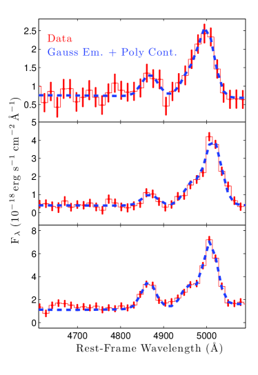
Figure 1.— Examples of the region about H$\beta$ and the [O III] doublet for three typical $z\sim 2$ COSMOS field galaxies observed with the WFC3 G141 grism of the 3D-HST program. From top to bottom, the three spectra represent below average, average, and better than average examples. The emission lines and underlying continuum were modeled with a Gaussian and polynomial, respectively.

3. Sample Selection and Measurements

We began our analysis by examining each 1-D extracted spectrum by eye to search for evidence of the emission lines of hydrogen (H$\alpha$ and H$\beta$), [O II] $\lambda 3727$, and [O III] $\lambda\lambda 4959,5007$. (Other commonly detected lines included [Ne III] $\lambda 3869$ and the [S II] blend at $\lambda\lambda 6716,6731$.) Spectra exhibiting two or more emission lines were inspected in more detail. Specifically, in the redshift range $1.90<z<2.35$, the bright lines of [O III], H$\beta$, [Ne III], and [O II] all fall within the coverage of the G141 grism. Moreover, the limited spectral resolution of the survey ($\sim 93$ Å) blends the [O III] $\lambda\lambda 4959,5007$ doublet together, creating a distinctive asymmetric profile (see Figure 1). As [O III] $\lambda 5007$ is typically the strongest emission line in these spectra, this was the most common feature selected for detailed inspection. Secure redshifts were determined if two or more emission lines provided a consistent redshift for the object. (The [O III] doublet counted as two lines, due to its unique shape.) In total, we visually inspected $>50,000$ spectra, and obtained redshifts for 323 $1.90<z<2.35$ galaxies with photometric coverage in the rest-frame UV.

Overlapping spectra are a significant issue in slitless spectroscopy: frequently, a portion of the dispersed order of one source will overlap the spectrum of another, causing “contamination.” To model this effect, we used the sizes and magnitudes of every object in the SExtractor catalog to create a 2-D Gaussian model of its expected spectrum (Kümmel et al., 2009). This map was then projected back onto the coordinate system of the science frame to create a contamination map of the region. Unfortunately, while this procedure is sufficient to identify most spectral superpositions, it does not identify or properly quantify all regions where the the systematics of contamination subtraction dominates the error in the continuum. In fact, a visual inspection of our sample of 323 $z\sim 2$ galaxies found 59 objects where the systematic error of contamination subtraction was greater than the statistical error of the target spectrum. These objects were removed from our sample along with four galaxies that are likely active galactic nuclei (see §3.4), leaving a total of 260 $1.90<z<2.35$ galaxies distributed over the three fields of GOODS-S, GOODS-N, and COSMOS.

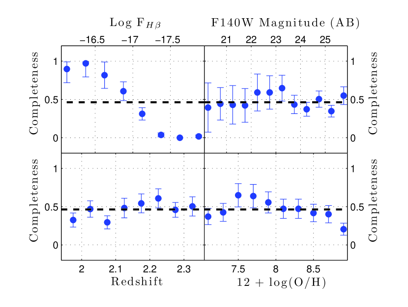
Figure 2.— Survey completeness and 1-$\sigma$ error bars as a function of H$\beta$ flux, continuum magnitude, redshift, and metallicity, as determined by a Monte Carlo experiment. The dashed line shows the total recovery rate for our experiment. Our recovery fraction is only a function of line flux, with the 50% completeness limit in the GOODS fields at $F_{{\rm H}\beta}\sim 10^{-17}$ ergs s^-1 cm^-2.

To understand our sample selection, we “observed” a set of simulated emission-line spectra in the exact same manner as our program data. To realistically model uncertainties produced by contamination, we began with the F140W magnitude and positional distributions defined in the master SExtractor catalog. We then randomly drew from a uniform distribution and assigned to each object a redshift ($1.90<z<2.35$), a metallicity ($7<12+\log({\rm O/H})<9$), and H$\beta$ flux (drawn from a uniform distribution in log space with $-18<\log F_{{\rm H}\beta}<-16$ ergs s^-1 cm^-2). For a given metallicity and H$\beta$ flux, it is possible to use locally-calibrated, strong line metallicity indicators to predict the line strengths for [O III], [Ne III], and [O II]. We used the polynomial relations in Table 4 and Equation 1 of Maiolino et al. (2008), which is discussed in more detail in §3.2, to convert metallicity and H$\beta$ flux into line strengths of [O III], [Ne III], and [O II]. These lines were superposed onto a constant flux density continuum that matched the object’s F140W magnitude. A total of 500 of these high-resolution template spectra were then placed onto a simulated grism image (and an accompanying direct image) using the aXeSim software package, and extracted in the same manner as the original data. A summary of this analysis is shown in Figure 2. From the figure, it is clear that our ability to detect and measure H$\beta$ is virtually independent of redshift, metallicity, and continuum magnitude. Formally, for the GOODS-N and GOODS-S fields, our 50% and 80% completeness limits for H$\beta$ are $\sim 10^{-17}$ ergs s^-1 cm^-2 and $\sim 3\times 10^{-17}$ ergs s^-1 cm^-2, respectively, with little variation across parameter space. Due to the higher background, the COSMOS limits are shallower by a factor of $\sim$ 1.5 (Brammer et al., 2012). Note that these 50% limits are roughly equivalent to the 1-$\sigma$ flux measurement found by Brammer et al. (2012). Our high recovery fraction is due principally to the fact that most of our galaxies were originally identified via the presence of much stronger emission lines, such as the [O III] doublet and [O II] $\lambda 3727$. This allows for the identification and measurement of H$\beta$ to much lower flux limits than would be possible based on blind detection of H$\beta$.

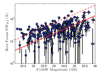
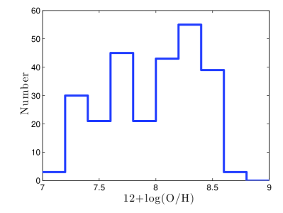
Figure 3.— Left: The rest-frame H$\beta$ equivalent widths (Å) plotted against continuum AB magnitude for our sample of $z\sim 2$ sources. The solid red line is our 50% completeness limit $F_{{\rm H}\beta}\sim 10^{-17}$ ergs s^-1 cm^-2, while the red dashed line shows our 80% completeness limit, $F_{{\rm H}\beta}\sim 3\times 10^{-17}$ ergs s^-1 cm^-2. All equivalent widths were calculated using the measured flux of H$\beta$, the continuum magnitude measured on the direct F140W frame, and the redshift. We include 1-$\sigma$ error bars for each measurement.Right: Distribution of the best-fit gas-phase metallicities ($12+\log{\rm(O/H)}$) from Gebhardt et al. (2014).

3.1. H$\beta$ Luminosity

The H$\beta$ line luminosities were determined by fitting the continuum of each $z\sim 2$ spectrum with a fourth-order polynomial, while simultaneously fitting Gaussians of a common width and redshift to the emission lines of [O II] $\lambda 3727$, [Ne III] $\lambda 3869$, H$\gamma$, H$\beta$, [O III] $\lambda 4959$, and [O III] $\lambda 5007$. The fourth-order polynomial was used due to the possible presence of a 4000 Å break. However, we also fit first-order polynomials and Gaussians in small wavelength windows for [O II], [NeIII], H$\gamma$, and the combination of H$\beta$ and [O III] due to their proximity. Both methods yielded consistent results. Example fits around H$\beta$ and the [O III] doublet are shown in Figure 1. These line fluxes were then increased by 5% to compensate for the fact that our grism extraction apertures (which were typically $2\arcsec$ to $4\arcsec$ in diameter) enclosed only 93% to 97% of the spectral flux for a point source. The galaxies in our sample are not point sources but are small compared to the extraction aperture, with typical half-light radii of 0.25-0.50″ (Hagen et al., 2014), indicating that our correction for extraction aperture flux loss is appropriate. Finally, these total H$\beta$ fluxes were converted to luminosity using the standard cosmology stated in the introduction.

Note that we do not correct for underlying stellar absorption, which can affect determinations of the star formation rate (Moustakas et al., 2006). In the local universe, typical corrections for Balmer absorption are $\sim 4$ Å in equivalent width (EW), but this number is a function of both the stellar population’s age and IMF (Groves et al., 2012). Moreover, as seen in Figure 3, 4 Å  is relatively small compared to the measured equivalent widths of our objects. Indeed, to verify that the effect is minor, we repeated all our analyses while statistically adding 4 Å EW to each of our H$\beta$ measurements. This has the effect of increasing all our H$\beta$ fluxes by an average of $\sim 10\%$, and increasing the significance of our findings.

3.2. Gas-Phase Metallicity

In addition to providing measurements of total luminosity, our Gaussian fits to [O II], [Ne III], H$\beta$, and [O III] also allow the measurement of every system’s gas phase metallicity, $12+\log{\rm(O/H)}$. The details of this analysis can be found in Gebhardt et al. (2014) including a catalog of the sources in this work, but in brief, we used the observed flux ratios and the polynomial relations in Table 4 of Maiolino et al. (2008) to estimate metallicity via the abundance sensitive diagnostics of [Ne III] to [O II], [O III] to [O II], and $R_{23}$ (([O III] + [O II]) / H$\beta$) (Zaritsky et al., 1994). These estimates should be relatively reliable, as they mate the $T_{e}$ “direct” methods, which are applicable to systems with $12+\log({\rm O/H})<8.35$ to the photo-ionization models of Kewley & Dopita (2002), which are useful for $12+\log({\rm O/H})>8.35$. Some of these measures are relatively insensitive to extinction, while others are highly affected by reddening. To account for this effect, we adopted a Calzetti et al. (2000) extinction curve, and computed gas-phase metallicity likelihood functions for fixed $E(B-V)=0.2$. The most likely system metallicity was adopted for our analysis. Some abundance indicators, such as $R_{23}$, are double-valued, and many of our likelihood curves have two local maxima. Fortunately, the use of the other diagnostics, such as [Ne III] to [O II] and [O III] to [O II], helped split this degeneracy, and usually led to the preference of one solution over the other. To verify that our fixed extinction value did not affect our results, we repeated our following analysis using all possible values of reddening ($0<E(B-V)<2$), and then marginalized over this uniform reddening distribution to derive the gas-phase metallicity likelihood function. The most likely system metallicities for all reddenings did not change our conclusions, only increased our metallicity error bars. The distribution of our best-fit metallicities is shown in on the right side of Figure 3.

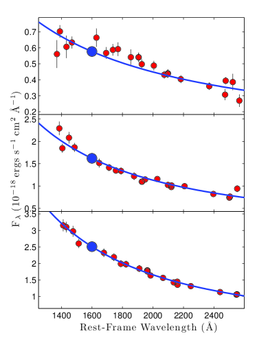
Figure 4.— Three examples of the photometric data available for the COSMOS and GOODS-S fields. From top to bottom, the three UV spectral energy distributions represent below average, average, and better than average spectral energy distributions. The red points show the measured flux densities with their associated uncertainties, the blue curve displays the best-fit power slope, and the large blue dot represents the best-fit flux density at 1600 Å. Typically, for $z\sim 2$ galaxies, the rest-frame UV between 1250 and 2600 Å is covered by $\gtrsim 15$ photometric bands; this allows us to accurately measure both the slope and normalization of the UV continuum.

3.3. UV Luminosity and Slope

To obtain the rest-frame UV flux densities of our sources, we used the photometric catalogs produced by Skelton et al. (2014). For star-forming populations, the wavelength range between $1250~{}{\rm\AA}<\lambda<2600$ Å samples the Rayleigh-Jeans portion of the hot stars’ spectral energy distributions. Consequently, in the absence of reddening, the spectral slope across this region should be relatively constant, i.e.,

$$F(\lambda)\propto\lambda^{\beta}$$ (1)

where $\beta\sim-2.25$ for systems which have been forming stars at a constant rate for more than $\sim 10^{8}$ yr (Calzetti, 2001). Values of $\beta$ larger than $-2.25$ can be attributed to the effects of internal extinction, and, if the law of Calzetti (2001) holds, $A_{1600}\sim 2.31\,\Delta\beta$.

As Figure 4 illustrates, the photometry covering our program’s fields is quite extensive (Skelton et al., 2014). In the COSMOS field, broad- and intermediate-band measurements constitute a set of $\sim 19$ data points which can be fit for $\beta$ and the observed flux density at 1600 Å . These bands include g, r, and i from CFHT (Erben et al., 2009; Hildebrandt et al., 2009), B_J, V_J, r+, i+ and 11 intermediate bands from Subaru (Taniguchi et al., 2007; Ilbert et al., 2009), and F606W from HST/ACS (Grogin et al., 2011; Koekemoer et al., 2011). In the GOODS-S field, there are $\sim 20$ data points covering the wavelength range $1250~{}{\rm\AA}<\lambda_{\rm rest}<2600$ Å. These include B, V, R_c and I from the WFI 2.2m (Erben et al., 2005; Hildebrandt et al., 2006), R from VLT/VIMOS (Nonino et al., 2009), 12 intermediate bands from Subaru (Cardamone et al., 2010), and F435W, F606W, and F775W from HST/ACS (Giavalisco et al., 2004; Grogin et al., 2011; Koekemoer et al., 2011). Photometry in the GOODS-N field is not nearly so comprehensive, but it does include $\sim 9$ data points in the $z\sim 2$ rest-frame UV. These include G and R_S from Keck/LRIS (Steidel et al., 2003), B_J, V_J, R, and i from Subaru (Capak et al., 2004), and F435W, F606W, and F775W from HST/ACS (Giavalisco et al., 2004; Grogin et al., 2011; Koekemoer et al., 2011). Since the PSF-matched apertures of the Skelton et al. (2014) photometric catalog are corrected for flux losses based on high-resolution imaging (HST/WFC3 F160W or F140W) at roughly the same wavelength as our grism observations, they serve as a good match to the total H$\beta$ fluxes provided by our grism measurements.

While complications may arise if the reddening curves contain a Milky-Way type bump at $\sim 2175$ Å, a careful examination of the COSMOS and GOODS-S photometry reveals no evidence for such a feature. This result is consistent with previous analyses, which have shown the bump to be less pronounced or non-existent in high equivalent-width objects such as those being studied (e.g., Kriek & Conroy, 2013).

3.4. AGN Rejection

Strong emission lines may be excited by the ionizing photons of hot stars, shocks in the ISM, and/or active galactic nuclei (AGN). In the local universe, diagnostic line ratios work quite well in discriminating between these mechanisms (e.g., Baldwin et al., 1981; Kewley et al., 2013), but at $z\sim 2$, key lines such as H$\alpha$ and [S II] $\lambda\lambda 6716,6731$ shift out of the range of the WFC3 grism. Fortunately, there are medium and deep X-ray data over all three of our program fields (Elvis et al., 2009; Alexander et al., 2003; Xue et al., 2011). At the redshifts considered here ($1.90<z<2.35$), the X-rays associated with normal star formation are well below the limits of these surveys (Lehmer et al., 2010). Consequently any emission-line galaxy whose position lies co-incident with an X-ray source is likely powered by an AGN.

To identify the AGN, we therefore cross-correlated our $z\sim 2$ object catalog with the list of X-ray sources found in the COSMOS, GOODS-N, and GOODS-S regions. Only four of our emission-line galaxies lie within $2.5\arcsec$ of an X-ray source; these objects have been removed from our sample.

While we cannot exclude the possibility that low-luminosity AGN are contributing flux to our survey, we can place limits on their effect. To do this, we converted the flux limits of the three X-ray surveys covering our fields (Elvis et al., 2009; Alexander et al., 2003; Xue et al., 2011) into a 2 KeV luminosity density ($L_{\rm 2KeV}$) using a power-law index of 1.9 and the online conversion tool, PIMMS. For AGN, there is a strong correlation between $L_{\rm 2KeV}$ and the luminosity density at 2500Å, $L_{2500}$. We therefore used equation 6 in Lusso et al. (2010) to convert the $L_{\rm 2KeV}$ limits into the maximum contribution “normal” AGN have to $L_{2500}$ . We then assumed a power-law slope of $\alpha=-0.5$ (i.e. L${}_{\nu}\propto\nu^{\alpha}$; Vanden Berk et al., 2001) to convert $L_{2500}$ to $L_{1600}$ as well as $L_{4861}$. With an extra assumption that for AGN, the H$\beta$ equivalent width is typically $\sim$100 Å (Binette et al., 1993), we were able to estimate the maximal contribution AGN have on the observed UV and H$\beta$ luminosities. This can be seen in Figure 5. For GOODS-N and GOODS-S, AGN have very little effect on either luminosity measurement and can be neglected. For COSMOS, the maximal AGN contribution to the UV and H$\beta$ luminosities is less than or roughly equal to the median observed values, and the ratio of the contribution to $L_{{\rm H}\beta}$ to $L_{1600}$ is roughly what is expected from normal star-forming galaxies. After excluding the individual X-ray sources from our analysis, it is clear that remaining AGN have very little effect on the observed UV and H$\beta$ luminosities and thus do not change our following SFR analysis.

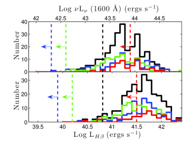
Figure 5.— The maximal AGN contribution to the observed H$\beta$ luminosity (bottom panel) and the observed UV continuum luminosity (top panel). The distributions for GOODS-S, GOODS-N, COSMOS, and the combined dataset are displayed in blue, green, red, and black, respectively. The dashed vertical lines illustrate that maximum contribution from AGN, and are based on the X-ray flux limits of the three survey fields (Elvis et al., 2009; Alexander et al., 2003; Xue et al., 2011), an X-ray to optical power-law index of 1.9, and a rest-frame UV power-law slope of $\alpha=-0.5$. For reference, the black dashed vertical line shows a SFR of $1M_{\odot}$ yr^-1 (Hao et al., 2011; Murphy et al., 2011). After excluding X-ray point sources from our analysis, we find that any remaining AGN must have very little effect on the observed distributions of UV and H$\beta$ luminosities.

4. Star Formation Rates

4.1. Results

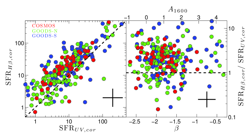
Figure 6.— A comparison of the H$\beta$ and UV star formation rates, using the SFR conversions of Hao et al. (2011) and Murphy et al. (2011) (summarized in Kennicutt & Evans, 2012) and a Calzetti (2001) extinction law. The left panel shows the extinction-corrected SFRs for COSMOS (red), GOODS-N (green), and GOODS-S (blue); the right panel displays the ratio of these two measurements as a function of the UV continuum slope. The typical 1-$\sigma$ uncertainties are shown as crosses. On average, the H$\beta$ SFR is $\sim 1.8$ times that of the UV rate. This result does not depend on internal extinction.

Two of the most common tracers of star formation are the UV continuum and the hydrogen recombination lines (e.g., H$\beta$). Both quantities are sensitive to the existence of short-lived, massive stars, but their systematics are different. The ultraviolet continuum at 1600 Å measures the photospheric emission of stars with masses greater than a few $M_{\odot}$, hence the method records star formation over a time scale of $\sim 100$ Myr. In contrast, the recombination lines of hydrogen are powered by photons shortward of 13.6 eV, with

$$L_{{\rm H}\beta}=Q({\rm H}^{0})\left(\frac{{\alpha}^{\rm eff}_{\rm H\beta}}{{\alpha}_{B}}\right)h{\nu}_{{\rm H}\beta}\approx 4.81\times 10^{-13}\ Q({\rm H}^{0})\ {\rm ergs\ s^{-1}}~{},$$ (2)

where ${\alpha}_{B}$ and ${\alpha}^{\rm eff}_{\rm H\beta}$ are the recombination coefficients for Case B and H$\beta$, respectively (Pengelly, 1964; Osterbrock & Ferland, 2006). This number is virtually independent of temperature, density, and metallicity; the luminosity of H$\beta$ only depends on the production rate of ionizing photons ($Q$), and the assumption that the interstellar medium is optically thick in the Lyman continuum. Since the stars that produce these ionizing photons have higher masses ($M\gtrsim 15~{}M_{\odot}$) and shorter lifetimes ($t\lesssim 10$ Myr) than the stars traced by the rest-frame UV, the exact relationship between the two star formation rate indicators can be complicated. In particular, variables such as the IMF, the stellar metallicity, and the history of star formation can all effect the observed ratio of the indicators.

The most common transformations between luminosity and star formation rate are those given by Kennicutt (1998) and updated by Kennicutt & Evans (2012). These conversions, which were originally tabulated in Hao et al. (2011) and Murphy et al. (2011), are based on results from the STARBURST99 population synthesis code (Leitherer et al., 1999; Vázquez & Leitherer, 2005), and assume a constant star formation history, solar metallicity, a Kroupa (2001) IMF, and a stellar population age of 10⁸ years. Using these relations, along with the assumption of Case B recombination with an intrinsic H$\alpha$/H$\beta$ ratio of 2.86 (Brocklehurst, 1971; Osterbrock & Ferland, 2006), a galaxy’s star formation rate can be inferred from

$$\log~{}{\rm SFR}_{\rm H\beta}=\log L_{\rm H\beta}-40.81~{}(M_{\odot}~{}{\rm yr}^{-1}),$$ (3)

$$\log~{}{\rm SFR}_{\rm UV}=\log L_{UV}-43.35~{}(M_{\odot}~{}{\rm yr}^{-1}),$$ (4)

where $L_{\rm H\beta}$ and $L_{UV}$ represent the total luminosities of H$\beta$ and the UV continuum, after correcting for interstellar extinction.

This last issue can be problematic. According to Calzetti (2001), in the local universe, the total extinction (in magnitudes) at 1600 Å is related to the slope of the UV continuum via

$$A_{1600}=\kappa_{\beta}\times(\beta-{\beta}_{0}),$$ (5)

where $\kappa_{\beta}=2.31$, and $\beta_{0}=-2.25$ for populations that have been forming stars for more than $\sim 10^{8}$ yr. The connection between $\beta$ and the extinction of the H$\beta$ emission line is more tenuous, but again from Calzetti (2001)

$$A_{\rm H\beta}=\zeta_{{\rm H}\beta}\,A_{1600}$$ (6)

with $\zeta_{{\rm H}\beta}=0.83$. We begin by adopting these coefficients in our analysis, and then test for variations by examining the systematics of the inferred star formation rates.

Figure 6 compares the H$\beta$ and UV star formation rates for our sample of 260 $1.90<z<2.35$ galaxies in the COSMOS, GOODS-N, and GOODS-S regions. From the figure, it is clear that the relations summarized in Kennicutt & Evans (2012), which typically produce a one-to-one correspondence in the $z\sim 0$ universe (at least for SFR $\gtrsim 10^{-2}M_{\odot}$ yr^-1; see Lee et al., 2009), do not work as well at $z\sim 2$. On average, H$\beta$ star formation rates are $\sim 1.8$ times higher than those derived from the flux of the rest-frame UV. Moreover, this effect cannot simply be attributed to extinction, as there is no correlation between the H$\beta$/UV SFR ratio and the value of $\beta$. To identify the source of the discrepancy, we need to examine the effects that various assumptions have on the derived SFRs.

4.2. Stellar Population Modeling

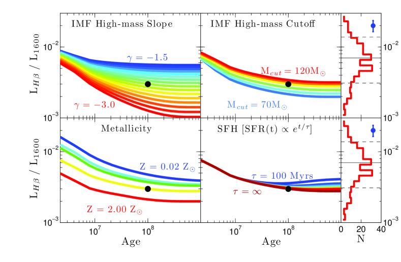
Figure 7.— The ratio of H$\beta$ luminosity to the luminosity density at 1600 Å as a function of age for a variety of STARBURST99 models. The large black points represent the calibration model of Hao et al. (2011) and Murphy et al. (2011) (summarized in Kennicutt & Evans, 2012), which assumes an IMF slope of $\gamma=-2.3$ (Salpeter, 1955; Kroupa, 2001), an upper mass cutoff of $100M_{\odot}$, solar metallicity, and a constant star formation history. The various panels show the effect of changing the IMF (from $\gamma=-3.0$ to $-1.5$ in units of 0.1), the high-mass cutoff (from $70M_{\odot}$ to $120M_{\odot}$ in units of $10M_{\odot}$), the population metallicity (with $0.02Z_{\odot}$, $0.20Z_{\odot}$, $0.40Z_{\odot}$, $1.00Z_{\odot}$, and $2.00Z_{\odot}$), and star formation history (with exponentially increasing $e$-folding time scales between $100~{}{\rm Myr}<\tau<1$ Gyr in intervals of 100 Myr). A constant SFR model ($\tau=\infty$) is also presented. The right-hand panels display the histogram of $L_{{\rm H}\beta}/L_{1600}$ for our sample of $z\sim 2$ star-forming galaxies, with the average 1-$\sigma$ error bar shown in blue. The solid black horizontal line represents the median of the sample while the lower and upper dashed black lines are the 16^th and 84^th percentiles.

To model the systematics of the Balmer line and UV SFR indicators, we began with the assumptions that no ionizing photons are escaping into the intergalactic medium, and that dust in the H II regions has, at most, a minor effect on the conversion of far-UV radiation to H$\beta$. The former assertion is probably quite good: at $z\sim 3$, the escape fraction of Lyman continuum photons is certainly less than 20%, and probably below $\sim$ 5% (Chen et al., 2007; Iwata et al., 2009; Vanzella et al., 2010; Mostardi et al., 2013), and observations in the local universe suggest $f_{\rm esc}<1\%$ (Adams et al., 2011). The latter assumption is also justifiable. Enshrouding dust exists for only a short period of time before O stars evaporate or evacuate it (Lada & Lada, 2003), and the dust that does survive likely affects the UV and the Lyman continuum in roughly equal proportions. In the metal-rich H II regions of the Milky Way, $\sim 25\%$ of far-UV photons may be absorbed by dust (see Table 3 of McKee & Williams, 1997), but in the metal-poor systems of the $z\sim 2$ universe, this fraction is likely to be much less. We therefore believe that this is not a large effect, and we can proceed to translate stellar emission into the observables of H$\beta$ and $L_{1600}$.

We examined the response of $L_{{\rm H}\beta}$ and $L_{\rm UV}$ to changes in stellar population by first adopting as the baseline model of Hao et al. (2011) and Murphy et al. (2011) (summarized in Kennicutt & Evans, 2012) SFR calibration, which uses solar metallicity, a Kroupa (2001) IMF, an upper mass cutoff of $100M_{\odot}$, and a constant star formation history. We then varied these parameters one at a time, using Version 6.0.4 of the STARBURST99 (Leitherer et al., 1999; Vázquez & Leitherer, 2005; Leitherer et al., 2010) population synthesis code with its Padova isochrones. Figure 7 displays the results, which we discuss below. This procedure is similar and consistent with previous works, albeit for H$\alpha$ to UV, which investigated the ratio produced by different IMFs (e.g., Meurer et al., 2009), stellar metallicities (e.g., Lee et al., 2009), and star formation histories (e.g., Sullivan et al., 2000).

4.2.1 Initial Mass Function

The IMF is usually assumed to be universal and power-law in form for masses $M>M_{\odot}$. As H$\beta$ and the UV are sensitive to different ranges of this function, their predicted luminosity ratio will depend on the slope of the power-law ($\gamma$) and its upper mass cutoff ($M_{\rm cut}$). Varying these two parameters within a reasonable range can change the predicted $L_{{\rm H}\beta}-L_{1600}$ ratio by a factor of two or more.

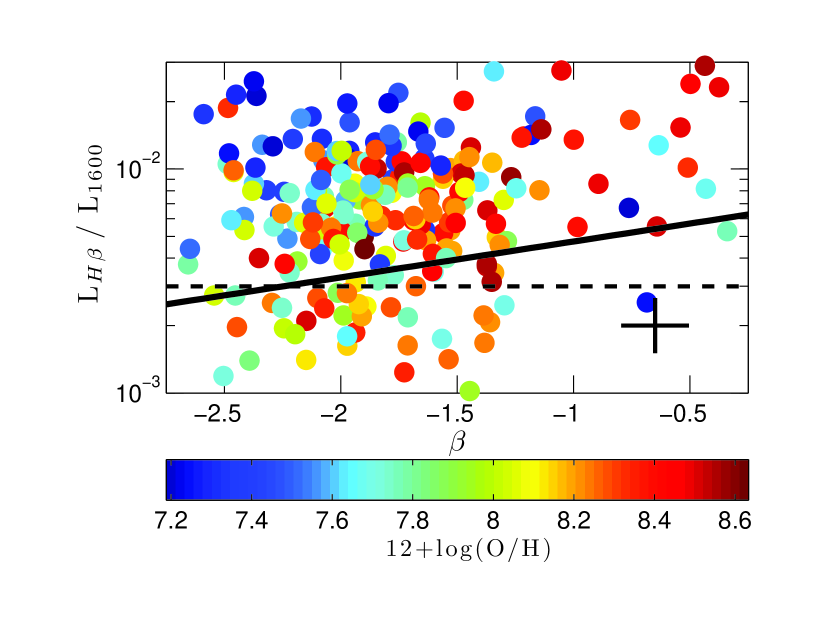
Figure 8.— The observed ratio of H$\beta$ luminosity to UV luminosity at 1600 Å (before correcting for reddening) as a function of continuum slope in the rest-frame UV. The data points are colored by their best-fit gas-phase metallicity ($12+\log{\rm O/H}$) and illustrate a correlation between metallicity and reddening, with the metal-rich systems being dustier. A representative 1-$\sigma$ error bar is shown in the bottom right corner. The dashed horizontal black line shows the value of $L_{{\rm H}\beta}/L_{1600}$ expected from the SFR calibrations of Hao et al. (2011) and Murphy et al. (2011), which are summarized in Kennicutt & Evans (2012). The solid black line couples these calibrations with the relation between $A_{1600}$ and H$\beta$ extinction detailed by Calzetti (2001). The anticipated anti-correlation between metallicity and $L_{{\rm H}\beta}/L_{\rm UV}$ is weak, but present.

The top two panels of Figure 7 demonstrate this behavior. As expected, a flatter IMF implies relatively greater numbers of high-mass stars, and hence higher values for the $L_{{\rm H}\beta}/L_{1600}$. In the Milky Way, $\gamma\sim-2.3$ (Salpeter, 1955; Kroupa, 2001; Chabrier, 2003), and this is the value used by Hao et al. (2011) and Murphy et al. (2011) (summarized in Kennicutt & Evans, 2012) in their SFR calibrations. However, despite recent advances (see Offner et al., 2013, and references therein), a firm theoretical understanding of the physics of the IMF is still missing, thus its shape in $z\sim 2$ star-forming galaxies may be different. Similarly, if the upper-mass limit to the main sequence is higher in our $z\sim 2$ systems, it will increase the luminosity of H$\beta$ more than that of the rest-frame UV continuum.

4.2.2 Metallicity

The metallicity of a stellar population affects the ratio of H$\beta$ to UV luminosity through the opacity and line blanketing in higher mass stars. The lower the metallicity, the bluer the stellar population and the higher the ratio of $L_{{\rm H}\beta}$ to $L_{1600}$. This effect can be seen in the bottom left panel of Figure 7: as we change the metallicity of the population from 0.02 solar to twice solar, H$\beta$ becomes enhanced relative to the UV continuum. As demonstrated by Gebhardt et al. (2014), the gas-phase oxygen abundances for our sample of $z\sim 2$ galaxies range between $7.1<12+\log({\rm O/H})<8.7$ (i.e., $0.025\,Z_{\odot}<Z<Z_{\odot}$ with the solar calibration of Asplund et al., 2009), and the median value of the sample is $12+\log({\rm O/H})=8.06$ ($Z\sim 0.2Z_{\odot}$). Thus, for star formation time scales larger than $\sim 100$ Myr, we should expect a $\sim 30\%$ increase in the $L_{{\rm H}\beta}/L_{1600}$ ratio compared to that given by Hao et al. (2011) and Murphy et al. (2011).

Figure 8 displays the observed ratio of H$\beta$ to UV continuum luminosity as a function of $\beta$, with the galaxies color-coded by their best-fit gas-phase metallicity. An inspection of the figure suggests the existence of a strong positive correlation between galactic extinction (as measured by the slope of the UV continuum) and oxygen abundance. Indeed, a Spearman test confirms this trend, as it rejects the null hypothesis that the two variables are uncorrelated with 99.9999% confidence. Of course, a correlation between extinction and oxygen abundance makes sense, as the formation of dust should be tied to the presence of metals in the ISM (e.g., Garn & Best, 2010; Reddy et al., 2010). However, one would also expect a strong anti-correlation between metallicity and $L_{\rm H\beta}/L_{1600}$. Since both the UV and H$\beta$ are powered by the energy emitted from young stars, and the $L_{\rm H\beta}/L_{1600}$ ratio is sensitive to metallicity, one would expect the two parameters to vary inversely with each other. Indeed, the Spearman test rejects the null hypothesis with 99.8% confidence.

4.2.3 Star Formation History

Since H$\beta$ and the UV continuum are sensitive to different ranges of stellar mass, the age of the stellar population and the assumed star formation history are important for our analysis. In their calibration of star formation rate, Hao et al. (2011) and Murphy et al. (2011) assumed a constant star formation rate history over a time scale greater than $10^{8}$ Myr. To explore if this assumption is sufficient for our sample of galaxies, we examined the relationship between two proxies of specific star formation rate (sSFR): EW_Hβ and $\log L_{1600}-\log L_{1.45\mu m}$. The former should be proportional to the mass-to-light ratio at 4861 Å times the sSFR (see Equation 8 in Zeimann et al., 2013) while the latter weighs the newly formed population relative to the older, longer-lived stars. As shown in Figure 9, a constant star formation history over a suite of ages from 7 $\times$ 10⁶ years to 10⁹ years cover the range of extinction-corrected, rest-frame EW_Hβ as well as the extinction-corrected UV to IR color.

In the literature, models with a bursty star formation history have been explored extensively in order to explain the scatter or offsets in Balmer line to UV SFR ratios (e.g. Sullivan et al., 2000; Iglesias-Páramo et al., 2004; Erb et al., 2006; Meurer et al., 2009). The scatter in Figure 6 however, can be explained simply by the combination of measurement error and the uncertainty in the extinction-correction. In other words, we need not invoke bursts to explain the diagram. Moreover, the offset may be more simply explained by a range of ages for a constant star formation history. The relation between H$\beta$ and UV SFR asymptotes for ages larger than 10⁸ years, while for ages younger than that the H$\beta$ SFR will appear enhanced. Our selection method may preferentially select young or newly-formed galaxies, some of which may have ages less than 10⁸ years. If we equate our extinction-corrected, rest-frame EW_Hβ to an age using the models in Figure 9, we find that our sample selection biases the H$\beta$/UV SFR ratio by at most $\sim$10%.

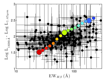
Figure 9.— The rest-frame equivalent width of H$\beta$ plotted against the rest-frame UV minus IR color for our 3D-HST sample of galaxies. Both quantities have been de-reddened using the relations of Calzetti (2001); $k$-corrections have been omitted, as these vary by less than 10% over the redshift range of the survey. Our 1-$\sigma$ error bars include measurement uncertainties and the propagation of errors associated with extinction-correction. The colored circles represent STARBURST99 models with constant star formation, a Kroupa IMF, $Z\sim 0.2Z_{\odot}$, and ages from $7\times 10^{6}$ yr (blue) to $10^{9}$ yr (red), logarithmically spaced. The larger circles in blue, yellow and red represent $10^{7}$, $10^{8}$, and $10^{9}$ yr, respectively. These constant star formation rate models extend the range of our data both in color and equivalent width.

Another consideration, as demonstrated by Maraston et al. (2010), is that galaxies at $z\sim 2$ are better modeled with an increasing star formation rate history, and this has a small effect on the predicted value of $L_{{\rm H}\beta}/L_{1600}$. As illustrated in the bottom right panel of Figure 7, an exponentially increasing star formation rate with an $e$-folding timescale of $\tau=300$ Myr will, over the course of a Gyr, increase $L_{{\rm H}\beta}/L_{1600}$ by $\sim 20\%$ over that of a constant star formation rate system. Similarly, if star formation has only recently ignited, H$\beta$ will again be boosted relative to the UV continuum. Consequently, unless galaxies at $z\sim 2$ already have declining star formation rates, the H$\beta$ to UV ratio predicted by the Kennicutt & Evans (2012) calibration should be a lower bound to the true value.

4.3. Dust

As nearly all stars form in clusters, the massive stars responsible for H$\beta$ and UV emission are initially co-located and enshrouded in high optical depth molecular clouds (Lada & Lada, 2003). As the stellar population ages, the most massive stars, which are primarily responsible for H$\beta$ emission, go supernovae and evacuate much of their surrounding interstellar material, leaving the longer-lived B stars relatively unobscured. Consequently, as noted many times in the literature (e.g., Charlot & Fall, 2000), there can be a systematic difference between the extinction that affects H$\beta$ and that which reddens the UV continuum. Moreover, this offset can be a function of age, star formation history, galactic orientation, and dust composition.

Charlot & Fall (2000) used a simple model of two separate environments, a birth cloud and a global ISM, to estimate the differential extinction seen by nebular emission and longer-lived stars. Meanwhile, Calzetti et al. (2000) inferred an empirical relation between stellar and nebular extinction using observations of eight nearby starburst systems. Both studies reached the same conclusion: in most systems, $A_{V}$ for the gas should be roughly twice that of the stars.

For $z\sim 2$ systems, the wavelength coverage of 3D-HST survey does not extend out to H$\alpha$, and the wavelength separation between H$\beta$ and the higher-order Balmer lines is insufficient to obtain a robust measure of extinction. However, we can measure the amount of extinction affecting the stars via the slope of the rest-frame UV continuum. STARBURST99 models confirm the results of Calzetti (2001) that stellar populations dominated by a roughly steady-state number of young stars will have values of $\beta$ between $-2.4$ and $-2.2$, depending on the time scale for the on-going star formation. Significantly, this number has little dependence on the IMF and stellar metallicity; any deviations from this intrinsic slope must either arise from dust attenuation or, to a smaller extent, the SFR history of the stellar population.

In fact, the relationship between the observed ratio of $L_{H\beta}/L_{1600}$ and $\beta$ can reveal more than just the extinction law. The data and axes of Figure 10 are identical to those of Figure 8, i.e., the figure plots the observed luminosities of H$\beta$ relative to the UV continuum, uncorrected for extinction. The best fit linear relation between this ratio and the slope of the UV continuum (as determined by unweighted least squares) is shown in red. The intercept of this line with $\beta\sim-2.3$ (i.e., where reddening should be minimal) provides information about the parameters of the underlying stellar population. Conversely, the slope of the line, $m$, constrains the ratio of nebular to UV extinction through

$$\log{(L_{\rm H\beta}/L_{UV})}=\log{(L_{\rm H\beta}/L_{UV})_{\rm int}}+m(\beta-\beta_{0}),$$ (7)

where,

$$m=0.4\times(1-\zeta_{{\rm H}\beta})\kappa_{\beta}~{}.$$ (8)

As is illustrated in the figure, the intercept of the line with $\beta\sim-2.3$ is inconsistent with the SFR calibrations of Hao et al. (2011) and Murphy et al. (2011), as summarized in Kennicutt & Evans (2012), at the 99.9995% confidence level. More specifically, $(L_{{\rm H}\beta}/L_{UV})_{\rm int}$ is $1.84^{+0.17}_{-0.17}$ larger than in the local universe, where the uncertainties represent 68% confidence intervals. Conversely, the slope of the relation, $m=0.155\pm 0.043$ is perfectly consistent with the value of 0.162 expected from a Calzetti (2001) extinction law. It therefore appears that at $z\sim 2$, $A_{V}$ for the gas is still approximately twice that of the stars.

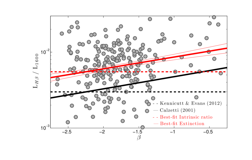
Figure 10.— As in Figure 8, the observed ratio of H$\beta$ to UV luminosity (uncorrected for extinction) is plotted against the slope of the rest-frame UV continuum. The black dashed line shows the expected ratio from Hao et al. (2011) and Murphy et al. (2011), as summarized in Kennicutt & Evans (2012), and the solid black line couples this number with the Calzetti (2001) extinction law so that the slope $m=0.4\times(1-\zeta_{{\rm H}\beta})\kappa_{\beta}=0.162$. The thick red line represents the best-fit linear regression, while the thinner red lines illustrate the 68% confidence limits. The intercept of this line with the zero-reddening value $\beta\sim-2.3$ demonstrates that $L_{{\rm H}\beta}/L_{\rm UV}$ is $1.84^{+0.17}_{-0.17}$ greater than that inferred from Hao et al. (2011) and Murphy et al. (2011), thus excluding the local calibration with 99.9995% confidence. This $z\sim 2$ zero-point is shown via the dashed red line. Conversely, the slope of the best-fit line is $0.155\pm 0.043$, which is consistent with Calzetti (2001). For reference, lower values for the slope indicate a larger differential extinction between gas and dust.

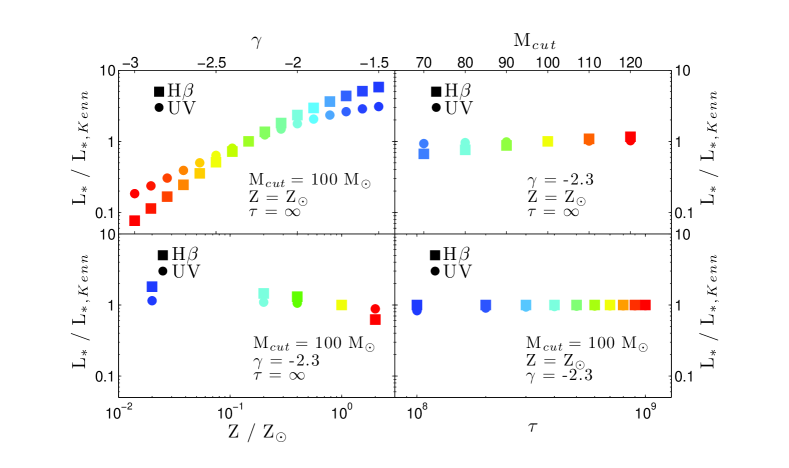
Figure 11.— The H$\beta$ (squares) and UV (circles) star formation rates compared to those predicted using the SFR calibrations of Hao et al. (2011) and Murphy et al. (2011), as summarized in Kennicutt & Evans (2012). The colors are the same as Figure 7, and the age of the stellar population is 10⁸ years for all panels. Values of $L_{*}/L_{*,{\rm Kenn}}$ greater than one imply that the Kennicutt & Evans (2012) relations will overestimate the true SFR, while values less than one indicate underestimates. As in Figure 7, the top left panel varies the slope of the IMF, the top right panel shows the response to changes in the high-mass cutoff, the bottom left panel varies metallicity, and the bottom right panel changes the $e$-folding time scale for star formation. These calculations were performed with the STARBURST99 population synthesis code, and do not include extinction. In general, the strength of the hydrogen recombination lines is more sensitive to population parameters than the rest-frame UV.

5. Discussion

A wide range of methods are used for determining SFRs in different fields of astronomy. Studies in the Local Group or the Milky Way galaxy may infer the star formation rate from the number of sources found in a molecular complex or H II region via deep observations in the infrared or X-ray. As each system may be in a different phase of evolution, and have different external conditions and population parameters, the results of these studies can be quite diverse (Chomiuk & Povich, 2011). In contrast, an extragalactic astronomer usually measures star formation over galaxy-wide scales, and must average over many of these differences. Indeed, given the wide range of properties observed for the star-forming complexes of the Milky Way (Feigelson et al., 2013) it is surprising the degree of consistency that most SFR indicators exhibit, especially when the total SFR energy budget is well-tracked (Calzetti et al., 2007; Kennicutt & Evans, 2012).

In the local volume (out to 11 Mpc), UV and Balmer-line SFRs have been measured for a complete set of galaxies extending all the way down to $M_{B}\lesssim-15$ (Lee et al., 2009). In these systems, measurements of the Balmer decrement and the total infrared luminosity have enabled independent determinations of both the nebular and stellar reddening, thus allowing both SFR indicators to be tested in a variety of environments. Interestingly, these data show that the SFR indicators summarized in Kennicutt & Evans (2012) do well in systems with SFRs greater than $\sim 0.01M_{\odot}$ yr^-1, but below this threshold, the relation over-predicts the Balmer lines (Lee et al., 2009). Explanations for this offset include a variable IMF (e.g., Meurer et al., 2009; Boselli et al., 2009; Pflamm-Altenburg et al., 2009), stochasticity (Fumagalli et al., 2011), non-constant star formation histories (Weisz et al., 2012), and leakage of ionizing photons into the intergalactic medium (Relaño et al., 2012). Interestingly, this deficit for very low SFR systems is the exact opposite of what is seen at $z\sim 2$, where H$\beta$ is enhanced relative to the UV continuum. This suggest that very low SFRs in the local sample may be masking the effect metallicity has on the ratio. Unfortunately, as these SFRs are inaccessible for 3D-HST, a direct test of this hypothesis is not possible. Still, it does indicate tension between observations and expectations.

At high redshift, information from multiple indicators and constraints on extinction are limited. For this reason most high-$z$ studies simply assume the SFR calibrations of the local universe (e.g., Kennicutt, 1998; Kennicutt & Evans, 2012) and then allow the extinction law to float, as this is the most uncertain aspect of the analysis (e.g., Daddi et al., 2007; Förster Schreiber et al., 2009; Wuyts et al., 2013). The extinction that forces agreement between the Balmer line and UV SFRs is then adopted. Not surprisingly, the results from such experiments at $1<z<3$ have varied. Some studies have found that extinction for the stars and gas are roughly equal, or, using the formalism of this paper, $\zeta_{{\rm H}\beta}=0.46$ (e.g., Erb et al., 2006). Others analyses have concluded that the Balmer-line gas is typically extinguished roughly twice as much as the stars, and follows a Calzetti (2001) law with $E(B-V)_{\rm stars}=0.44\times E(B-V)_{\rm gas}$, or $\zeta_{{\rm H}\beta}=1.05$ (e.g., Förster Schreiber et al., 2009; Mannucci et al., 2009; Holden et al., 2014). Still others suggest that the true relation is somewhere in between (e.g., Wuyts et al., 2013; Price et al., 2013). If we re-fit our data in Figure 10 while restricting the $y$-intercept at $\beta=-2.25$ to match the SFR relations summarized in Kennicutt & Evans (2012) and use $\kappa_{\beta}=1.99-2.31$ (Meurer et al., 1999; Calzetti, 2001), then we obtain $\zeta_{{\rm H}\beta}=0.76-0.88$. This is consistent with the intermediate case, where the gas is more extinguished than the stars but not twice as much.

However, SFR calibrations must be treated with caution (e.g., Kennicutt, 1983; Kennicutt et al., 1994; Kennicutt et al., 2009). Assumptions about the IMF, star formation history, and population metallicity all play a role in the transformation of observables into estimates of star formation. For example, Figure 11 uses the results of our STARBURST99 models to demonstrate how H$\beta$ and the rest-frame UV continuum luminosity each respond to changes in the commonly used assumptions that go into estimating SFRs. The slope of the high-mass end of the initial mass function has the greatest effect on our measurements. Yet this parameter still lacks a theoretical understanding (see Offner et al., 2013, and references there within), and is essentially unconstrained at $z\sim 2$. More tractable is the response of the SFR to changes in metallicity. As shown in Figure 11, the rest-frame UV is rather robust to shifts in the metal abundance, as a population with $0.02\,Z_{\odot}$ will only be $\sim 15$% brighter than a corresponding solar-metallicity system. In contrast, the H$\beta$ luminosity of such a metal-poor population will be larger by almost a factor of two, leading to a clear overestimate of the star formation rate. Previous works that have taken metallicity into account when calculating SFR (e.g., Lee et al., 2002; Brinchmann et al., 2004; Hunter & Elmegreen, 2004) have found similar results. Table 1 summarizes this fact by listing correction factors to the SFR relations summarized in Kennicutt & Evans (2012) as a function of metallicity. For our 3D-HST sample, the gas-phase metallicities indicate a correction of $-0.16$ and $-0.04$ dex for our H$\beta$ and UV SFRs, respectively. When this factor is applied to the data, the expected $L_{{\rm H}\beta}$-$L_{\rm UV}$ ratio lies just outside of the 98% confidence interval of Figure 10. Other corrections, such as that associated with an increasing star formation rate history, also make the expected intrinsic luminosity more consistent with the data.

Table 1SFR Corrections

$Z/Z_{\odot}$	Balmer emission	FUV
0.02	$-$0.26	$-$0.06
0.20	$-$0.16	$-$0.04
0.40	$-$0.12	$-$0.02
1.00	$+$0.00	$+$0.00
2.00	$+$0.21	$+$0.05

Note. — Additive logarithmic corrections to the SFR calibrations of Hao et al. (2011), Murphy et al. (2011), and Kennicutt & Evans (2012).

6. Summary

We use near-IR spectroscopy from 3D-HST and a wealth of photometric data in the GOODS-S, GOODS-N, and COSMOS fields to compare the H$\beta$ and rest-frame UV extinction-corrected SFRs of 260 galaxies in the redshift range $1.90<z<2.35$. Compared to the values expected from the UV luminosity density, our H$\beta$ SFRs are a factor of $\sim 1.8$ times higher than expected. The lower metallicity of these $z\sim 2$ systems accounts for some of this offset, as models suggest that H$\beta$ should be enhanced by $\sim 45\%$, compared to only $\sim 10\%$ for the rest-frame UV. Also, if star formation has only recently ignited, H$\beta$ will be elevated relative to the UV continuum. Future IR spectroscopic surveys of $z>2$ star forming systems will need to take these factors into account when interpreting their data.

Our observations also demonstrate that, as for the starburst galaxies of the local universe, the dust in these $z\sim 2$ star forming systems extinguishes the stellar UV continuum more than optical emission lines. While the H$\beta$ and UV observations alone are insufficient to define the extinction law of these systems, we can determine a product which includes the total extinction at 1600 Å and the ratio H$\beta$ to UV extinction. Obviously, measurements of the Balmer decrement can break this degeneracy, but even without these additional expensive observations, it is clear that our data are in excellent agreement with a Calzetti (2001) extinction law. This result supports the premise that measurements of the rest-frame UV slope in $z\sim 2$ star-forming systems can be used to estimate nebular reddening.

References

- Adams et al. (2011) Adams, J.J., Uson, J.M., Hill, G.J., & MacQueen, P.J. 2011, ApJ, 728, 107
- Alexander et al. (2003) Alexander, D.M., Bauer, F.E., Brandt, W.N., et al. 2003, AJ, 126, 539
- Asplund et al. (2009) Asplund, M., Grevesse, N., Sauval, A.J., & Scott, P. 2009, ARA&A, 47, 481
- Baldwin et al. (1981) Baldwin, J.A., Phillips, M.M., & Terlevich, R. 1981, PASP, 93, 5
- Bertin & Arnouts (1996) Bertin, E., & Arnouts, S. 1996, A&AS, 117, 393
- Binette et al. (1993) Binette, L., Fosbury, R. A., & Parker, D. 1993, PASP, 105, 1150
- Boselli et al. (2009) Boselli, A., Boissier, S., Cortese, L., et al. 2009, ApJ, 706, 1527
- Brammer et al. (2012) Brammer, G.B., van Dokkum, P.G., Franx, M., et al. 2012, ApJS, 200, 13
- Brinchmann et al. (2004) Brinchmann, J., Charlot, S., White, S. D. M., et al. 2004, MNRAS, 351, 1151
- Brocklehurst (1971) Brocklehurst, M. 1971, MNRAS, 153, 471
- Calzetti et al. (2000) Calzetti, D., Armus, L., Bohlin, R.C., et al. 2000, ApJ, 533, 682
- Calzetti (2001) Calzetti, D. 2001, PASP, 113, 1449
- Calzetti et al. (2007) Calzetti, D., Kennicutt, R.C., Engelbracht, C.W., et al. 2007, ApJ, 666, 870
- Capak et al. (2004) Capak, P., Cowie, L. L., Hu, E. M., et al. 2004, AJ, 127, 180
- Cardamone et al. (2010) Cardamone, C.N., van Dokkum, P.G., Urry, C.M., et al. 2010, ApJS, 189, 270
- Chabrier (2003) Chabrier, G. 2003, PASP, 115, 763
- Charlot & Fall (2000) Charlot, S., & Fall, S.M. 2000, ApJ, 539, 718
- Chen et al. (2007) Chen, H.-W., Prochaska, J.X., & Gnedin, N.Y. 2007, ApJ, 667, L125
- Chomiuk & Povich (2011) Chomiuk, L., & Povich, M.S. 2011, AJ, 142, 197
- Daddi et al. (2007) Daddi, E., Dickinson, M., Morrison, G., et al. 2007, ApJ, 670, 156
- Dressel et al. (2014) Dressel, L. 2014, Wide Field Camera 3 Instrument Handbook, Version 6.0 (Baltimore: STScI)
- Elvis et al. (2009) Elvis, M., Civano, F., Vignali, C., et al. 2009, ApJS, 184, 158
- Erb et al. (2006) Erb, D.K., Steidel, C.C., Shapley, A.E., et al. 2006, ApJ, 647, 128
- Erben et al. (2005) Erben, T., Schirmer, M., Dietrich, J. P., et al. 2005, Astronomische Nachrichten, 326, 432
- Erben et al. (2009) Erben, T., Hildebrandt, H., Lerchster, M., et al. 2009, A&A, 493, 1197
- Feigelson et al. (2013) Feigelson, E.D., Townsley, L.K., Broos, P.S., et al. 2013, ApJS, 209, 26
- Ford et al. (2003) Ford, H.C., Clampin, M., Hartig, G.F., et al. 2003, Proc. SPIE, 4854, 81
- Förster Schreiber et al. (2009) Förster Schreiber, N.M., Genzel, R., Bouché, N., et al. 2009, ApJ, 706, 1364
- Fruchter et al. (2009) Fruchter, A., Sosey, M., Hack, W., et al. 2009, The MultiDrizzle Handbook Version 3.0 (Baltimore, STScI)
- Fumagalli et al. (2011) Fumagalli, M., da Silva, R.L., & Krumholz, M.R. 2011, ApJ, 741, L26
- Garn & Best (2010) Garn, T., & Best, P. N. 2010, MNRAS, 409, 421
- Gebhardt et al. (2014) Gebhardt, H., Zeimann, G.R., Ciardullo, R., & Gronwall, C. 2014, in preparation
- Giavalisco et al. (2004) Giavalisco, M., Ferguson, H.C., Koekemoer, A.M., et al. 2004, ApJ, 600, L93
- Grogin et al. (2011) Grogin, N.A., Kocevski, D.D., Faber, S.M., et al. 2011, ApJS, 197, 35
- Groves et al. (2012) Groves, B., Brinchmann, J., & Walcher, C.J. 2012, MNRAS, 419, 1402
- Guo et al. (2013) Guo, Y., Ferguson, H.C., Giavalisco, M., et al. 2013, ApJS, 207, 24
- Hagen et al. (2014) Hagen, A., Zeimann, G.R., Ciardullo, R., & Gronwall, C. 2014, in preparation
- Hao et al. (2011) Hao, C.N., Kennicutt, R.C., Johnson, B.D., et al. 2011, ApJ, 741, 124
- Hildebrandt et al. (2006) Hildebrandt, H., Erben, T., Dietrich, J. P., et al. 2006, A&A, 452, 1121
- Hildebrandt et al. (2009) Hildebrandt, H., Pielorz, J., Erben, T., et al. 2009, A&A, 498, 725
- Holden et al. (2014) Holden, B.P., Oesch, P.A., Gonzalez, V.G., et al. 2014, submitted to ApJ (arXiv:1401.5490)
- Hunter & Elmegreen (2004) Hunter, D. A., & Elmegreen, B. G. 2004, AJ, 128, 2170
- Iglesias-Páramo et al. (2004) Iglesias-Páramo, J., Boselli, A., Gavazzi, G., & Zaccardo, A. 2004, A&A, 421, 887
- Ilbert et al. (2009) Ilbert, O., Capak, P., Salvato, M., et al. 2009, ApJ, 690, 1236
- Iwata et al. (2009) Iwata, I., Inoue, A.K., Matsuda, Y., et al. 2009, ApJ, 692, 1287
- Kennicutt (1983) Kennicutt, R. C., Jr. 1983, ApJ, 272, 54
- Kennicutt et al. (1994) Kennicutt, R. C., Jr., Tamblyn, P., & Congdon, C. E. 1994, ApJ, 435, 22
- Kennicutt (1998) Kennicutt, R.C., Jr. 1998, ARA&A, 36, 189
- Kennicutt et al. (2009) Kennicutt, R.C., Jr., Hao, C.N., Calzetti, D., et al. 2009, ApJ, 703, 1672
- Kennicutt & Evans (2012) Kennicutt, R.C., & Evans, N.J. 2012, ARA&A, 50, 531
- Kewley & Dopita (2002) Kewley, L. J., & Dopita, M. A. 2002, ApJS, 142, 35
- Kewley et al. (2013) Kewley, L.J., Dopita, M.A., Leitherer, C., et al. 2013, ApJ, 774, 100
- Koekemoer et al. (2011) Koekemoer, A. M., Faber, S. M., Ferguson, H. C., et al. 2011, ApJS, 197, 36
- Kriek & Conroy (2013) Kriek, M., & Conroy, C. 2013, ApJ, 775, L16
- Kroupa (2001) Kroupa, P. 2001, MNRAS, 322, 231
- Kümmel et al. (2009) Kümmel, M., Walsh, J.R., Pirzkal, N., Kuntschner, H., & Pasquali, A. 2009, PASP, 121, 59
- Lada & Lada (2003) Lada, C.J., & Lada, E.A. 2003, ARA&A, 41, 57
- Lee et al. (2002) Lee, J. C., Salzer, J. J., Impey, C., Thuan, T. X., & Gronwall, C. 2002, AJ, 124, 3088
- Lee et al. (2009) Lee, J.C., Gil de Paz, A., Tremonti, C., et al. 2009, ApJ, 706, 599
- Lehmer et al. (2010) Lehmer, B.D., Alexander, D.M., Bauer, F.E., et al. 2010, ApJ, 724, 559
- Leitherer et al. (1999) Leitherer, C., Schaerer, D., Goldader, J.D., et al. 1999, ApJS, 123, 3
- Leitherer et al. (2010) Leitherer, C., Ortiz Otálvaro, P.A., Bresolin, F., et al. 2010, ApJS, 189, 309
- Lusso et al. (2010) Lusso, E., Comastri, A., Vignali, C., et al. 2010, A&A, 512, A34
- Madau et al. (1996) Madau, P., Ferguson, H.C., Dickinson, M.E., et al. 1996, MNRAS, 283, 1388
- Maiolino et al. (2008) Maiolino, R., Nagao, T., Grazian, A., et al. 2008, A&A, 488, 463
- Mannucci et al. (2009) Mannucci, F., Cresci, G., Maiolino, R., et al. 2009, MNRAS, 398, 1915
- Maraston et al. (2010) Maraston, C., Pforr, J., Renzini, A., et al. 2010, MNRAS, 407, 830
- McKee & Williams (1997) McKee, C.F., & Williams, J.P. 1997, ApJ, 476, 144
- Meurer et al. (1999) Meurer, G.R., Heckman, T.M., & Calzetti, D. 1999, ApJ, 521, 64
- Meurer et al. (2009) Meurer, G.R., Wong, O.I., Kim, J.H., et al. 2009, ApJ, 695, 765
- Mostardi et al. (2013) Mostardi, R.E., Shapley, A.E., Nestor, D.B., et al. 2013, ApJ, 779, 65
- Moustakas et al. (2006) Moustakas, J., Kennicutt, R. C., Jr., & Tremonti, C. A. 2006, ApJ, 642, 775
- Murphy et al. (2011) Murphy, E.J., Condon, J.J., Schinnerer, E., et al. 2011, ApJ, 737, 67
- Nonino et al. (2009) Nonino, M., Dickinson, M., Rosati, P., et al. 2009, ApJS, 183, 244
- Offner et al. (2013) Offner, S.S.R., Clark, P.C., Hennebelle, P., et al. 2013, in Protostars and Planets VI, eds. H. Beuther, et al.(Tucson: University of Arizona Press), in press (arXiv:1312.5326)
- Oke & Gunn (1983) Oke, J.B., & Gunn, J.E. 1983, ApJ, 266, 713
- Osterbrock & Ferland (2006) Osterbrock, D.E., & Ferland, G.J. 2006, Astrophysics of Gaseous Nebulae and Active Galactic Nuclei, 2nd. ed. by D.E. Osterbrock & G.J. Ferland (Sausalito, CA: University Science Books)
- Pengelly (1964) Pengelly, R.M. 1964, MNRAS, 127, 145
- Pflamm-Altenburg et al. (2009) Pflamm-Altenburg, J., Weidner, C., & Kroupa, P. 2009, MNRAS, 395, 394
- Price et al. (2013) Price, S.H., Kriek, M., Brammer, G.B., et al. 2013, submitted to ApJ (arXiv:1310.4177)
- Reddy et al. (2010) Reddy, N. A., Erb, D. K., Pettini, M., Steidel, C. C., & Shapley, A. E. 2010, ApJ, 712, 1070
- Relaño et al. (2012) Relaño, M., Kennicutt, R.C., Jr., Eldridge, J.J., Lee, J.C., & Verley, S. 2012, MNRAS, 423, 2933
- Salpeter (1955) Salpeter, E.E. 1955, ApJ, 121, 161
- Scoville et al. (2007) Scoville, N., Aussel, H., Brusa, M., et al. 2007, ApJS, 172, 1
- Skelton et al. (2014) Skelton, R. E., Whitaker, K. E., Momcheva, I. G., et al. 2014, (arXiv:1403.3689)
- Steidel et al. (2003) Steidel, C. C., Adelberger, K. L., Shapley, A. E., et al. 2003, ApJ, 592, 728
- Sullivan et al. (2000) Sullivan, M., Treyer, M. A., Ellis, R. S., et al. 2000, MNRAS, 312, 442
- Taniguchi et al. (2007) Taniguchi, Y., Scoville, N., Murayama, T., et al. 2007, ApJS, 172, 9
- Tinsley (1980) Tinsley, B.M. 1980, Fund. Cosmic Phys., 5, 287
- Vanzella et al. (2010) Vanzella, E., Giavalisco, M., Inoue, A.K., et al. 2010, ApJ, 725, 1011
- Vanden Berk et al. (2001) Vanden Berk, D. E., Richards, G. T., Bauer, A., et al. 2001, AJ, 122, 549
- Vázquez & Leitherer (2005) Vázquez, G.A., & Leitherer, C. 2005, ApJ, 621, 695
- Weisz et al. (2012) Weisz, D.R., Johnson, B.D., Johnson, L.C., et al.2012, ApJ, 744, 44
- Wuyts et al. (2013) Wuyts, S., Förster Schreiber, N.M., Nelson, E.J., et al. 2013, ApJ, 779, 135
- Xue et al. (2011) Xue, Y.Q., Luo, B., Brandt, W.N., et al. 2011, ApJS, 195, 10
- Zaritsky et al. (1994) Zaritsky, D., Kennicutt, R.C., Jr., & Huchra, J.P. 1994, ApJ, 420, 87
- Zeimann et al. (2013) Zeimann, G. R., Stanford, S. A., Brodwin, M., et al. 2013, ApJ, 779, 137