Generalized characteristic polynomials and Gaussian cubature rules

Abstract.

For a family of near banded Toeplitz matrices, generalized characteristic polynomials are shown to be orthogonal polynomials of two variables, which include the Chebyshev polynomials of the second kind on the deltoid as a special case. These orthogonal polynomials possess maximal number of real common zeros, which generate a family of Gaussian cubature rules in two variables.

1. Introduction

Characteristic polynomials for non-square matrices are defined and studied in [1], which can be viewed as the multidimensional generalization of the usual characteristic polynomials. We describe a connection between these polynomials and multivariate orthogonal polynomials, which leads to a family of orthogonal polynomials in two variables that has maximal number of real distinct common zeros. The latter serve as nodes of a new family of Gaussian cubature rules.

We start with the definition of generalized characteristic polynomials. For $m,n\in{\mathbb{N}}$, let ${\mathcal{M}}(m,n)$ denote the space of complex valued matrices of size $m\times n$ and let ${\mathcal{M}}(n)={\mathcal{M}}(n,n)$. For $A\in{\mathcal{M}}(n)$, the eigenvalues of $A$ are the zeros of the characteristic polynomial $\det(x{\mathcal{I}}_{n}-A)$, where ${\mathcal{I}}_{n}$ denotes the identity matrix in ${\mathcal{M}}(n)$. The notion of the characteristic polynomial has been extended to several variables in [1, 10]. For $s=0,1,\ldots,n$ define the $s$-unit matrix

$${\mathcal{I}}_{s}:=(\delta_{s+i-j})\in{\mathcal{M}}(m,m+n).$$

As an example, for $n=1$, ${\mathcal{I}}_{0}=[{\mathcal{I}}_{m}\,0]$ and ${\mathcal{I}}_{1}=[0\,\,{\mathcal{I}}_{m}]$. Let $A$ be a matrix in ${\mathcal{M}}(m,m+n)$. Define the $m\times(m+n)$ matrix

$$A(z_{0},\ldots,z_{n}):=A+z_{0}{\mathcal{I}}_{0}+\ldots+z_{n}{\mathcal{I}}_{n}.$$

For $I=\{i_{1},\ldots,i_{m}\}$, where $1\leq i_{1}<\cdots<i_{m}\leq m+n$, denote by $A_{I}(z_{0},\ldots,z_{n})$ the submatrix of $A(z_{0},\ldots,z_{n})$ formed by its $m$ columns indexed by $I$. The generalized characteristic polynomials of $A$ are then defined by

(1.1) $$P_{I}(z_{0},\ldots,z_{n}):=\det A_{I}(z_{0},\ldots,z_{n}).$$

Let $|I|$ denote the cardinality of $I$. It is easy to see that the total degree of $P_{I}(z_{0},\ldots,z_{n})$ is $|I|$. Furthermore, for $m\in{\mathbb{N}}_{0}$, there are $\binom{m+n}{m}$ polynomials $P_{I}(z_{0},\ldots,z_{n})$ with $|I|=m$ and these polynomials are linearly independent. Moreover, the following proposition was proved in [1].

Proposition 1.1.

The set of common zeros of all $P_{I}(z_{0},\ldots,z_{n})$ with $|I|=m$ is a finite subset of ${\mathbb{C}}^{n+1}$ of cardinality $\binom{m+n}{n+1}$ counting multiplicities.

The set of common zeros of $\binom{m+n}{n+1}$ randomly selected polynomials can be empty. The significance of the above scheme is that it gives a simple construction that warrants a maximal set of finite common zeros.

We are interested in the connection of these characteristic polynomials and orthogonal polynomials of several variables. For this purpose, we consider, for example, an infinite dimensional matrix ${\mathcal{A}}$ and define its $m$-th characteristic polynomials in terms of its main $m\times(m+n)$ submatrix (in the left and upper corner). In the case of one variable, characteristic polynomials satisfy a three–term relation if ${\mathcal{A}}$ is tri-diagonal with positive off–diagonal elements, which implies that they are orthogonal polynomials by Favard’s theorem. For several variables, it was pointed out in [1, Example 8] that if ${\mathcal{A}}$ is a Toeplitz matrix ${\mathcal{A}}=(c_{i-j})$ with $c_{-1}=c_{d}=1$ and all other $c_{i}=0$, then the generalized characteristic polynomials are, up to a change of variable, the Chebyshev polynomials of the second kind associated to the root system of ${\mathcal{A}}_{d}$ type ([2, 5]). These Chebyshev polynomials are orthogonal with respect to a real–valued weight function $w$ on a compact domain $\Omega\in{\mathbb{R}}^{d}$ (both $w$ and $\Omega$ are explicitly known) and they have been extensively studied ([2, 4, 8] and the references therein).

Together with Proposition 1.1, this suggests a way to find orthogonal polynomials that have maximal number of common zeros, which is related to the existence of Gaussian cubature rules. The latter is important for numerical integration and a number of other problem in orthogonal polynomials of several variables. Let $\Pi_{m}^{d}$ denote the space of real-valued polynomials of (total) degree $m$ in $d$ variables. For a given integral $\int_{{\mathbb{R}}^{d}}f(x)d\mu$, a cubature rule of degree $M$ in ${\mathbb{R}}^{d}$ with $N$ nodes is a finite sum of function evaluations such that

$$\int_{{\mathbb{R}}^{d}}f(x)d\mu=\sum_{k=1}^{N}{\lambda}_{k}f(x_{k}),\qquad x_{k}\in{\mathbb{R}}^{d},\quad{\lambda}_{k}\neq 0,$$

for all $f\in\Pi_{M}^{d}$, where $x_{k}$ are called nodes and ${\lambda}_{k}$ are called weights. It is known that the number of nodes, $N$, satisfies

$$N\geq\dim\Pi_{m-1}^{d}=\binom{m+d-1}{m},\qquad\hbox{$M=2m-1$ or $2m-2$}.$$

A cubature rule of degree $M=2m-1$ with $N$ attaining the above lower bound is called a Gaussian cubature rule. For $d=1$, a Gaussian quadrature rule of degree $2m-1$ always exists and its nodes are zeros of orthogonal polynomials of degree $m$ with respect to $d\mu$. For $d>1$, it is known that a Gaussian cubature rule of degree $2m-1$ exists if and only if the corresponding orthogonal polynomials of degree $m$ have $\binom{m+d-1}{m}$ real, distinct common zeros ([4, 9, 11]). As a consequence, Gaussian cubature rules rarely exist. In fact, at the moment, only two families of integrals are known for which Gaussican cubature rules of all orders exist ([3, 8]); one of them is generated by the Chebyshev polynomials of the second kind that are related to the generalized characteristic polynomials.

The purpose of this paper is to explore possible connection between characteristic polynomials and orthogonal polynomials, especially the connection that will lead to new Gaussian cubature rules. In order to establish that a family of generalized characteristic polynomials are orthogonal, we shall show that the polynomials satisfy a three–term relation which implies, by Favard’s theorem, orthogonality provided that the coefficients of the three–term relation satisfy certain conditions. Unlike the case of one variable, the three–term relation in several variables is given in vector form and its coefficients are matrices, which are more difficult for explicit computation. For this reason, we will primarily be working with polynomials of two variables. Our main result shows that there are a one–parameter perturbations of the Chebyshev polynomials of the second kind that are generalized characteristic polynomials, whose common zeros are all real, distinct, and generate Gaussian cubature rules.

In the next section, we provide background properties of orthogonal polynomials in several variables. Since we consider integrals in real variables for cubature rules and generalized characteristic polynomials are in complex variables, we need to work with polynomials in conjugate complex variables, which requires us to restate several results on orthogonal polynomials accordingly. In Section 3, we discuss generalized characteristic polynomials and two conjectures in [1] in greater detail, and we will explore the impact of the restriction to conjugate complex variables for these polynomials. The new orthogonal polynomials and Gaussian cubature rules are studied in Section 4.

2. Orthogonal polynomials and their common zeros

Let $\Pi_{n}^{d}$ denote the space of real–valued polynomials of degree at most $n$ in $d$ variables as before. Let $d\mu$ be a real–valued measure defined on a domain $\Omega\in{\mathbb{R}}^{d}$. We usually consider orthogonal polynomials with respect to the inner product

$${\langle}f,g{\rangle}_{\mu}:=\int_{\Omega}f(x)g(x)d\mu(x).$$

In some cases, we need to define orthogonal polynomials in terms of a linear functional, which is somewhat more general. Let ${\mathcal{L}}$ be a linear functional that has all finite moments. A polynomial $P\in\Pi_{n}^{d}$ is called an orthogonal polynomial with respect to ${\mathcal{L}}$ if ${\mathcal{L}}(PQ)=0$ for all polynomials $Q\in\Pi_{n-1}^{d}$. When ${\mathcal{L}}$ is defined by ${\mathcal{L}}f=\int_{\Omega}f(x)d\mu$, then this is the same as orthogonality with respect to ${\langle}f,g{\rangle}_{\mu}$. We will need the notion that ${\mathcal{L}}$ is positive definite and quasi–definite, see [4, Chapt. 3] for definition. For our purpose, the quasi definiteness allows us to use the Gram–Schmidt process to generate a complete sequence of orthogonal polynomials $\{P_{\alpha}:|{\alpha}|=n,{\alpha}\in{\mathbb{N}}_{0}^{d},n=0,1,2\ldots\}$, and the positive definiteness allows us to further normalize the basis to be an orthonormal one, that is, ${\mathcal{L}}(P_{\alpha}^{n}P_{\beta}^{m})=\delta_{{\alpha},{\beta}}\delta_{m,n}$ for all ${\alpha},{\beta}\in{\mathbb{N}}_{0}^{d}$ and $m,n\in{\mathbb{N}}_{0}$. For $d=1$, the positive definiteness of ${\mathcal{L}}$ means that ${\mathcal{L}}f=\int fd\mu$ for a nonnegative Borel measure. For $d>1$, however, further restriction on ${\mathcal{L}}$ is needed for this to hold.

Assume that orthogonal polynomials with respect to a linear functional ${\mathcal{L}}$ exist. For $n=0,1,\ldots,$ let ${\mathcal{V}}_{n}^{d}$ be the space of orthogonal polynomials of degree exactly $n$. It is known that $\dim{\mathcal{V}}_{n}^{d}=\binom{n+d-1}{n}$ and a basis of ${\mathcal{V}}_{n}^{d}$ can be conveniently indexed by the multi–indices in $\{{\alpha}\in{\mathbb{N}}_{0}^{d}:|{\alpha}|=n\}$ with respect to a fixed order, say the lexicographical order. Let ${\mathbb{P}}_{n}:=\{P_{\alpha}^{n}:|{\alpha}|=n\}$ be a basis of ${\mathcal{V}}_{n}^{d}$, where $n$ denotes the total degree of the polynomials. With respect to the fixed order, we can regard ${\mathbb{P}}_{n}$ as a column vector. The orthogonal polynomials satisfy a three–term relation, which takes the form of

(2.1) $$x_{i}{\mathbb{P}}_{n}(x)=A_{n,i}{\mathbb{P}}_{n+1}(x)+B_{n,i}{\mathbb{P}}_{n}(x)+C_{n,i}{\mathbb{P}}_{n-1}(x),\quad 1\leq i\leq d,$$

in the vector notation, where the coefficients $A_{n,i}$, $B_{n,i}$ and $C_{n,i}$ are real matrices of appropriate dimensions. These relations and a full rank assumption on $A_{n,i}$ in fact characterize the orthogonality. Furthermore, the polynomials in ${\mathbb{P}}_{n}$ have $\dim\Pi_{n-1}^{d}$ common zeros if and only if

(2.2) $$A_{n-1,i}A_{n-1,j}^{\mathsf{t}}=A_{n-1,j}A_{n-1,i}^{\mathsf{t}},\qquad 1\leq i,j\leq d.$$

For further results in this direction, see [4].

As we mentioned in the introduction, we need to consider orthogonal polynomials in complex conjugate variables. Let $\Pi_{n}^{d}({\mathbb{C}})$ denote the space of polynomials of total degree $n$ in conjugated complex variables $z_{1},\ldots,z_{d}$, where $z_{j}=\overline{z_{d-j}}$, with complex coefficients. If $d$ is odd, this requires $z_{\frac{d+1}{2}}\in{\mathbb{R}}$. The relation between the real and the complex variables are

$$x_{k}=\frac{1}{2}(z_{j}+z_{d-j}),\quad x_{d+1-k}=\frac{1}{2i}(z_{j}-z_{d-j})\quad 1\leq k\leq\lfloor\tfrac{d}{2}\rfloor,$$

and if $d$ is odd, then $x_{\frac{d+1}{2}}=z_{\frac{d+1}{2}}$. Let $d\mu$ be a real–valued measure defined on a domain $\Omega\in{\mathbb{R}}^{d}$. We define the orthogonality in terms of the inner product

$${\langle}f,g{\rangle}_{\mu}^{\mathbb{C}}:=\int_{\Omega}f(z_{1},z_{2},\ldots,\bar{z}_{2},\bar{z}_{1})\overline{g(z_{1},z_{2},\ldots,\bar{z}_{2},\bar{z}_{1})}d\mu$$

or its linear functional analogue. Let ${\mathcal{V}}_{n}^{d}({\mathbb{C}})$ denote the space of orthogonal polynomials of degree $n$ in $\Pi_{n}^{d}({\mathbb{C}})$ with respect to ${\langle}\cdot,\cdot{\rangle}_{\mu}^{\mathbb{C}}$. Since $d\mu$ is real–valued, it can be shown that ${\mathcal{V}}_{n}^{d}$ and ${\mathcal{V}}_{n}^{d}({\mathbb{C}})$ coincide. We can establish a precise correspondence between a basis in ${\mathcal{V}}_{n}^{d}$ and a basis $\{P_{\alpha}^{\mathbb{C}}:|{\alpha}|=n\}$ of ${\mathcal{V}}_{n}^{d}({\mathbb{C}})$ that satisfies the relation

(2.3) $$P_{\alpha}(z_{0},z_{1},\ldots,\bar{z}_{1},\bar{z}_{0})=\overline{P_{\alpha}(\bar{z}_{0},\bar{z}_{1}\ldots,z_{1},z_{0})}.$$

For orthogonal polynomials in conjugate complex variables, three–term relation and various properties that rely on the three–term relation take different forms. To state these results, we shall restrict to two variables, since this avoids complicated notations and our examples are given mostly in two variables.

For $d=2$, a basis of ${\mathcal{V}}_{n}^{2}$ contains $n+1$ elements, which can be conveniently denoted by $P_{k,n}(x,y)$, $0\leq k\leq n$, whereas a basis for ${\mathcal{V}}_{n}^{2}({\mathbb{C}})$ can be written as $P_{k,n}^{\mathbb{C}}(z,\bar{z})$. Let ${\mathbb{P}}_{n}^{\mathbb{C}}:=\{P_{0,n}^{\mathbb{C}},\ldots,P_{n,n}^{\mathbb{C}}\}$ and we regard it as a vector. The space ${\mathcal{V}}_{n}^{2}({\mathbb{C}})$ has many different bases, among which we can choose one that satisfies the relation ([12])

(2.4) $$\overline{{\mathbb{P}}_{n}^{\mathbb{C}}(z,\bar{z})}=J_{n+1}{\mathbb{P}}_{n}^{\mathbb{C}}(z,\bar{z}),\qquad J_{n}:=\left[\begin{matrix}\bigcirc&&1\\ &\mathinner{\mkern 1.0mu\raise 1.0pt\vbox{\kern 7.0pt\hbox{.}}\mkern 2.0mu\raise 4.0pt\hbox{.}\mkern 2.0mu\raise 7.0pt\hbox{.}\mkern 1.0mu}&\\ 1&&\bigcirc\end{matrix}\right],$$

where $J_{n}$ is of size $n\times n$, which is (2.3) for two complex variables. Furthermore, setting $z=x+iy$ and $\bar{z}=x-iy$, this basis and a basis for ${\mathcal{V}}_{n}^{2}$ are related by

(2.5) $$\begin{split}P_{k,n}(x,y)&:=\frac{1}{\sqrt{2}}\left[P^{\mathbb{C}}_{k,n}(z,\bar{z})+P^{\mathbb{C}}_{n-k,n}(z,\bar{z})\right],\quad 0\leq k\leq\frac{n}{2},\\ P_{k,n}(x,y)&:=\frac{1}{\sqrt{2}i}\left[P^{\mathbb{C}}_{k,n}(z,\bar{z})-P^{\mathbb{C}}_{n-k,n}(z,\bar{z})\right],\quad\frac{n}{2}<k\leq n.\end{split}$$

In the following we normalize our linear functionals so that ${\mathcal{L}}1=1$. We also define ${\mathbb{P}}_{0}^{\mathbb{C}}(z,\bar{z})=1$ and ${\mathbb{P}}^{\mathbb{C}}_{-1}(z,\bar{z})=0$.

In order to state the three–term relation for orthogonal polynomials in conjugate complex variables, we need one more definition. Let ${\mathcal{M}}^{\mathbb{C}}(n,m)$ denote the set of complex matrices of size $n\times m$. For a matrix $M\in{\mathcal{M}}^{\mathbb{C}}(n,m)$, we define a matrix $M^{\vee}$ of the same dimensions by

$$M^{\vee}:=J_{n}\overline{M}J_{m}.$$

The following is the three–term relation and the Favard’s theorem for polynomials in conjugate complex variables.

Theorem 2.1.

Let $\{{\mathbb{P}}^{\mathbb{C}}_{n}\}_{n=0}^{\infty}=\{P^{\mathbb{C}}_{k,n}:0\leq k\leq n,n\in{\mathbb{N}}_{0}\}$, ${\mathbb{P}}_{0}^{\mathbb{C}}(z,\bar{z})=1$, be an arbitrary sequence in $\Pi^{2}({\mathbb{C}})$. Then the following statements are equivalent.

1. There exists a quasi–definite linear functional ${\mathcal{L}}$ on $\Pi^{2}({\mathbb{C}})$ which makes $\{{\mathbb{P}}^{\mathbb{C}}_{n}\}_{n=0}^{\infty}$ an orthogonal basis in $\Pi^{d}({\mathbb{C}})$.

2. For $n\geq 0$, there exist matrices ${\alpha}_{n}:(n+1)\times(n+2)$, ${\beta}_{n}:(n+1)\times(n+1)$ and ${\gamma}_{n-1}:(n+1)\times n$ such that

   (2.6) $$z{\mathbb{P}}_{n}^{\mathbb{C}}(z,\bar{z}) ={\alpha}_{n}{\mathbb{P}}^{\mathbb{C}}_{n+1}(z,\bar{z})+{\beta}_{n}{\mathbb{P}}^{\mathbb{C}}_{n}(z,\bar{z})+{\gamma}_{n-1}{\mathbb{P}}^{\mathbb{C}}_{n-1}(z,\bar{z}),$$

   and the matrices in the relation satisfy the rank condition

   $$\operatorname{rank}({\alpha}_{n}+{\alpha}_{n}^{\vee}) =\operatorname{rank}({\alpha}_{n}-{\alpha}_{n}^{\vee})=n+1\quad\hbox{and}\quad\operatorname{rank}\left[\begin{matrix}{\alpha}_{n}\\ {\alpha}_{n}^{\vee}\end{matrix}\right]=n+2$$

   $$\operatorname{rank}({\gamma}_{n-1}+{\gamma}_{n-1}^{\vee}) =\operatorname{rank}({\gamma}_{n-1}-{\gamma}_{n-1}^{\vee})=n\quad\hbox{and}\quad\operatorname{rank}\left[\begin{matrix}{\gamma}_{n-1}\\ {\gamma}_{n-1}^{\vee}\end{matrix}\right]=n+1.$$

If ${\mathbb{P}}_{n}^{\mathbb{C}}$ is orthogonal, then the matrices ${\alpha}_{n}$ and ${\gamma}_{n-1}$ are related by

(2.7) $${\gamma}_{n-1}H_{n-1}=J_{n+1}({\alpha}_{n-1}H_{n})^{\mathsf{t}}J_{n}$$

where $H_{n}={\mathcal{L}}\big{(}{\mathbb{P}}^{\mathbb{C}}_{n}({\mathbb{P}}^{\mathbb{C}}_{n})^{*}\big{)}$. Using the fact that $J\overline{{\mathbb{P}}_{n}^{\mathbb{C}}}={\mathbb{P}}_{n}^{\mathbb{C}}$, it then follows from (2.6) that we also have

(2.8) $$\bar{z}{\mathbb{P}}_{n}^{\mathbb{C}}(z,\bar{z}) ={\alpha}_{n}^{\vee}{\mathbb{P}}^{\mathbb{C}}_{n+1}(z,\bar{z})+{\beta}_{n}^{\vee}{\mathbb{P}}^{\mathbb{C}}_{n}(z,\bar{z})+{\gamma}_{n-1}^{\vee}{\mathbb{P}}^{\mathbb{C}}_{n-1}(z,\bar{z}).$$

One can compare (2.6) and (2.8) with (2.1). These results were formulated recently in [12]. They can be deduced from (2.5) and the corresponding results in real variables, so are the results stated below.

Theorem 2.2.

The equivalence of Theorem 2.1 remains true if ${\mathcal{L}}$ is positive definite and ${\mathbb{P}}_{n}^{\mathbb{C}}$ are orthonormal in (1) and assume, in addition, that ${\gamma}_{n-1}=({\alpha}_{n-1}^{*})^{\vee}$ in (2). Furthermore, in this case, there is a real–valued positive measure $d\mu$ with compact support in ${\mathbb{R}}^{2}$ such that ${\mathcal{L}}f=\int fd\mu$ if

(2.9) $$\max_{n\geq 0}\|{\alpha}_{n}\|<\infty,\quad\hbox{and}\quad\max_{n\geq 0}\|{\beta}_{n}\|<\infty,\qquad n=0,1,2,\ldots,$$

where $\|\cdot\|$ is a fixed matrix norm.

The common zeros of ${\mathbb{P}}_{n}^{\mathbb{C}}$ can be characterized in terms of the coefficient matrices of the three–term relation. A common zero of ${\mathbb{P}}_{n}^{\mathbb{C}}$ is called simple if at least one partial derivative of ${\mathbb{P}}_{n}^{\mathbb{C}}$ is not identically zero.

Theorem 2.3.

Assume ${\mathbb{P}}_{n}^{\mathbb{C}}$ consists of an orthogonal basis of ${\mathcal{V}}_{n}^{2}({\mathbb{C}})$. Then

1. ${\mathbb{P}}^{\mathbb{C}}_{n}$ has $\dim\Pi_{n-1}^{2}$ common zeros if and only if

   (2.10) $${\alpha}_{n-1}{\gamma}_{n-1}^{\vee}={\alpha}_{n-1}^{\vee}{\gamma}_{n-1}.$$

2. If, in addition, ${\gamma}_{n-1}=({\alpha}_{n-1}^{*})^{\vee}$, then all zeros of ${\mathbb{P}}_{n}^{\mathbb{C}}$ are real.

3. All zeros of ${\mathbb{P}}_{n}^{\mathbb{C}}$ are simple.

For orthonormal polynomials, this result is stated in [12]; the above statement (without orthonormality) can be deduced form the results for orthogonal polynomials of real variables. We observe that, by Corollary 2.2, ${\gamma}_{n-1}=({\alpha}_{n-1}^{*})^{\vee}$ holds if ${\mathcal{L}}$ is positive definite, which holds if $H_{n}$ is positive definite for all $n\geq 0$. The condition (2.10) is equivalent to (2.2) and it does not usually hold.

Although the space of orthogonal polynomials of real variables and that of conjugate complex variables are the same, sometimes it is more convenient to work with conjugate complex variables. This is illustrated by the example below.

Example 2.4. Chebyshev polynomials on the deltoid. These polynomials are orthogonal with respect to

(2.11) $$w_{\alpha}(z):=\left[-3(x^{2}+y^{2}+1)^{2}+8(x^{3}-3xy^{2})+4\right]^{{\alpha}},\quad{\alpha}=\pm\frac{1}{2},$$

on the deltoid, which is a region bounded by the Steiner’s hypocycloid, or the curve

$$x+iy=(2e^{i{\theta}}+e^{-2i{\theta}})/3,\qquad 0\leq{\theta}\leq 2\pi.$$

The three–cusped region is depicted in Figure 1.

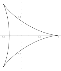
Figure 1. Region bounded by Steiner’s hypocycloid

These polynomials are first studied by Koornwinder in [5] and they are related to the symmetric and antisymmetric sums of exponentials on a regular hexagonal domain [7]. Let $U_{k}^{n}\in\Pi_{n}^{2}({\mathbb{C}})$ be the Chebyshev polynomials of the second kind defined by the three–term recursive relations

(2.12) $$U_{k}^{n+1}(z,\bar{z})=3zU_{k}^{n}(z,\bar{z})-U_{k+1}^{n}(z,\bar{z})-U_{k-1}^{n-1}(z,\bar{z})$$

for $0\leq k\leq n$ and $n\geq 1$, where $U_{-1}^{n}(z,\bar{z}):=0$ and $U_{n}^{n-1}(z,\bar{z}):=0$, and the initial conditions

$$U_{0}^{0}(z,\bar{z})=1,\quad U_{0}^{1}(z,\bar{z})=3z,\quad U_{1}^{1}(z,\bar{z})=3\bar{z}.$$

Then $U_{k}^{n}(z,\bar{z})$, $0\leq k\leq n$, are mutually orthogonal with respect to $w_{\frac{1}{2}}$. ∎

It is known ([7]) that the polynomials $U_{k}^{n}$, $0\leq k\leq n$, possess $\dim\Pi_{n-1}^{2}$ real common zeros and $w_{\frac{1}{2}}$ admits Gaussian cubature rule of degree $2n-1$ for all $n$.

3. Characteristic polynomials and orthogonal polynomials

In this section we discuss generalized characteristic polynomials defined in the introduction when the matrix $A$ is banded Toeplitz. In the case of one variable, it is well known that the characteristic polynomial of a tri–diagonal matrix with positive off–diagonal elements is an orthogonal polynomial with respect to some positive definite linear functional. For generalized characteristic polynomials to be orthogonal, we need more restrictive conditions on the matrix $A$, more or less a banded Toeplitz matrix.

Recall that, for a matrix $A\in{\mathcal{M}}(m,n+1)$ and $I=\{i_{1},\ldots,i_{m}\}$ for $1\leq i_{1}<\ldots<i_{m}\leq m+n$, the generalized characteristic polynomial $P_{I}(z_{0},\ldots,z_{n})$ is defined by (1.1) and it is a polynomials of degree $m$. If ${\mathcal{A}}$ is an infinite matrix, we define these polynomials for $A$ being the main $m\times(m+n)$ submatrix in the left and upper corner. We need the following definition from [6].

Definition 3.1.

A matrix $A\in{\mathcal{M}}(m,n)$ is called centrohermitian if

$$A=J_{m}\overline{A}J_{n}.$$

If $A=(a_{i,j})$ is a centrohermitian matrix in ${\mathcal{M}}_{m,m+n}$, then $a_{i,j}=\overline{a_{m+1-i,m+n+1-j}}$ for $1\leq i\leq m$ and $1\leq j\leq m+n$. If $n=2\ell$, then

$$A=\left[\begin{matrix}a_{1,1}&\cdots&a_{1,\ell}&\overline{a_{m,\ell}}&\cdots&\overline{a_{m,1}}\\ \vdots&\ddots&\vdots&\vdots&\ddots&\vdots\\ a_{m,1}&\cdots&a_{m,\ell}&\overline{a_{1,\ell}}&\cdots&\overline{a_{1,1}}\end{matrix}\right],$$

and if $n=2\ell+1$, then

$$A=\left[\begin{matrix}a_{1,1}&\cdots&a_{1,\ell}&a_{1,\ell+1}&\overline{a_{m,\ell}}&\cdots&\overline{a_{m,1}}\\ \vdots&\ddots&\vdots&\vdots&\vdots&\ddots&\vdots\\ a_{m,1}&\cdots&a_{m,\ell}&\overline{a_{1,\ell+1}}&\overline{a_{1,\ell}}&\cdots&\overline{a_{1,1}}\end{matrix}\right].$$

The following conjecture was made in [1]:

Conjecture 3.2.

If $A\in{\mathcal{M}}(m,m+n)$ is Toeplitz and centrohermitian, then each common zero $(z_{0},\ldots,z_{n})$ of $\{P_{I}:|I|=m\}$ satisfies $z_{j}=\overline{z_{n-j}}$, $0\leq j\leq n$.

The original conjecture used a more complicated notion, called multihermitian, see the arXiv version of [1], which was shown by the current author to be equivalent to the centrohermitian.

Proposition 3.3.

Let $A$ be a centrohermitian matrix in ${\mathcal{M}}(m,m+n)$. Then the polynomials $P_{I}$ in (1.1) satisfy the property

$$P_{\overline{I}}(z_{0},\ldots,z_{n})=\overline{P_{I}(\bar{z}_{n},\ldots,\bar{z}_{0})},$$

where $\overline{I}=m+n+1-I=\{m+n+1-i_{m},\ldots,m+n+1-i_{1}\}$.

Proof.

Directly from the centrohermitian of the matrix $A$, it follows that

$$\overline{A(z_{0},\ldots,z_{n})}=J_{m}A(\bar{z}_{n},\ldots,\bar{z}_{0})J_{m+n}.$$

Since multiplying $J_{m+n}$ from the right hand side reverse the order of the columns, we see that

$$\overline{A_{I}(z_{0},\ldots,z_{n})}=J_{m}A_{\overline{I}}(\bar{z}_{n},\ldots,\bar{z}_{0})J_{m},$$

from which the stated result for $P_{I}$ follows immediately. ∎

As a corollary of Proposition 3.3, we see that the polynomials $P_{I}$ associated with $A$ in the above proposition satisfies

$$\overline{P_{I}(z_{0},z_{1},\ldots,\overline{z}_{1},\overline{z}_{0})}=P_{\overline{I}}(z_{0},z_{1},\ldots,\overline{z}_{1},\overline{z}_{0}).$$

In particular, in the case of $d=2$, we can write $P_{I}$ as $P_{k,n}^{\mathbb{C}}$ for $0\leq k\leq n$ with $I=\{n-k,k\}$. Then the above relation coincides with (2.4). In view of this relation, we reformulate Conjecture 3.2 as follows:

Conjecture 3.4.

If $A\in{\mathcal{M}}(m,m+n)$ is Toeplitz and centrohermitian, then the common zeros $(z_{0},\ldots,z_{n})$ of $\{P_{I}(z_{0},z_{1},\ldots,\overline{z}_{1},\overline{z}_{0}):|I|=m\}$ are all real.

Our interest in real common zeros lies in the Gaussian cubature rules, for which we need characteristic polynomials to be orthogonal. Let us first consider the example of multivariate Chebyshev polynomials associated with the group ${\mathcal{A}}_{d}$. These Chebyshev polynomials are orthogonal and are extensively studied in the literature, see [2, 8] and the references therein. The three–term relations that they satisfy are explicitly given in [8], where it is also shown that these polynomials have maximal number of common zeros that serve as nodes for Gaussian cubature rules. In the case of $d=2$, the three–term relations are precisely those appearing in Example 2.4.

It was pointed out in [1, Example 8] that when ${\mathcal{A}}$ is the special Toeplitz matrix ${\mathcal{A}}=(c_{i-j})$ with $c_{-1}=c_{n+1}=1$ and all other $c_{j}=0$, the generalized characteristic polynomials are the multivariate Chebyshev polynomials associated with the group ${\mathcal{A}}_{n+1}$. This was stated in [1] without proof. In fact, the statement holds for a dilation of the characteristic polynomials and one way to prove it is to verify that the characteristic polynomials satisfy the same three–term relations of the multivariate Chebyshev polynomials. In the following we carry out this proof for the case of two variables, which will also be useful in the next section.

We consider, instead of $c=1$, more generally the matrix $A_{m,m+1}(z,\bar{z})$ defined by

$$A_{m,m+1}^{c}(z,\bar{z}):=\left[\begin{matrix}z&\bar{z}&\bar{c}&&&\bigcirc\\ c&z&\bar{z}&\bar{c}&&\\ &\ddots&\ddots&\ddots&\ddots&\\ &&c&z&\bar{z}&\bar{c}\\ \bigcirc&&&c&z&\bar{z}\end{matrix}\right]$$

and denote its generalized characteristic polynomials $P_{I}$ more conveniently by

$$P_{k}^{m}(z,\overline{z}),\quad 0\leq k\leq m,\quad\hbox{and}\quad{\mathbb{P}}_{m}=(P_{0}^{m},P_{1}^{m},\ldots,P_{m}^{m})^{\mathsf{t}},$$

where $P_{k}^{m}$ is the determinant of the matrix formed by $A_{m,m+1}^{c}(z,\bar{z})$ minus its $(m-k)$-th column. It is easy to see that $P_{k}^{m}(z,\bar{z})$ is monic; that is, its highest order monomial is $z^{m-k}\bar{z}^{k}$.

Proposition 3.5.

The polynomials defined above satisfy the three–term relation

(3.1) $$z{\mathbb{P}}_{m}(z,\overline{z})=[I_{m}\,\,0]{\mathbb{P}}_{m+1}(z,\overline{z})+{\beta}_{m}{\mathbb{P}}_{m}(z,\overline{z})+{\gamma}_{m}{\mathbb{P}}_{m-1}(z,\overline{z}),\quad m\geq 0$$

where

$${\beta}_{m}=\left[\begin{matrix}0&c&&\bigcirc\\ &\ddots&\ddots&\\ &&0&c\\ \bigcirc&&&0\end{matrix}\right]\quad\hbox{and}\quad{\gamma}_{m}=\left[\begin{matrix}0&\ldots&0\\ |c|^{2}&&\bigcirc\\ &\ddots&\\ \bigcirc&&|c|^{2}\end{matrix}\right].$$

Proof.

For $0\leq k\leq m$, define $k\times k$ matrices

$$A_{k}^{c}(z,\bar{z}):=\left[\begin{matrix}z&\bar{z}&\bar{c}&&&\bigcirc\\ c&z&\bar{z}&\bar{c}&&\\ &\ddots&\ddots&\ddots&\ddots&\\ &&c&z&\bar{z}&\bar{c}\\ &&&c&z&\bar{z}\\ \bigcirc&&&&c&z\end{matrix}\right],B_{k}^{c}(z,\bar{z}):=\left[\begin{matrix}\bar{z}&\bar{c}&&&&\bigcirc\\ z&\bar{z}&\bar{c}&&&\\ c&z&\bar{z}&\bar{c}&&\\ &\ddots&\ddots&\ddots&\ddots&\\ &&c&z&\bar{z}&\bar{c}\\ \bigcirc&&&c&z&\bar{z}\end{matrix}\right].$$

It follows directly from the definition that

$$P_{0}^{m}(z,\bar{z}) =\det A_{m}^{c}(z,\bar{z}),\quad P_{m}^{m}(z,\bar{z})=\det B_{m}^{c}(z,\bar{z}),$$

$$P_{k}^{m}(z,\bar{z}) =\det\left[\begin{array}[]{c|c}A_{m-k}^{c}(z,\bar{z})&\begin{matrix}&\bigcirc\\ \bar{c}\quad&\end{matrix}\\ \hline\cr\begin{matrix}&\qquad c\\ \bigcirc&\end{matrix}&B_{k}^{c}(z,\bar{z})\end{array}\right],\qquad 1\leq k\leq n-1.$$

Now, expanding the determinant of $P_{0}^{m}$ by the last row shows immediately that

$$P_{0}^{m}(z,\bar{z})=zP_{0}^{m-1}(z,\bar{z})-cP_{1}^{m-1}(z,\bar{z}).$$

Expanding the determinant in the first row for $P_{1}^{m}$ and the last row for $P_{2}^{m-1}$ leads to

$$P_{1}^{m}=zP_{1}^{m-1}-c\bar{z}P_{1}^{m-2}+c|c|^{2}P_{1}^{m-3},\quad P_{2}^{m-1}=\bar{z}P_{1}^{m-2}-\bar{c}zP_{0}^{m-2},$$

Combining these identities gives

$$P_{1}^{m}(z,\bar{z})=zP_{1}^{m-1}(z,\bar{z})-cP_{2}^{m-1}(z,\bar{z})-|c|^{2}P_{0}^{m-2}(z,\bar{z}).$$

The same process can be used to derive the expansion of $P_{k}^{m}(z,\bar{z})$, we omit the details. ∎

Corollary 3.6.

Let $c=\bar{a}^{3}/|a|^{2}$ and $U_{k}^{m}(z,\bar{z})=a^{-m+k}\bar{a}^{-k}P_{k}^{m}(3az,3\bar{a}\bar{z})$, $0\leq k\leq m$. Then the polynomials $U_{k}^{m}(az,\bar{a}\bar{z})$ are precisely the Chebyshev polynomials of the second kind defined in Example 2.4.

Proof.

Rewriting the three–term relation (3.1) in terms of $U_{k}^{m}$, it is easy to see that $U_{k}^{m}$ satisfy the three–term relation (2.12) and $U_{0}^{1}(z,\bar{z})=3z$ and $U_{1}^{1}(z,\bar{z})=3\bar{z}$. Since the three–term relation uniquely determines the system of polynomials, $U_{k}^{m}$ coincides with those defined in Example 2.4. ∎

In particular, when $c=a=1$, the characteristic polynomials $P_{k}^{m}(z,\bar{z})=U_{k}^{n}(z/3,\bar{z}/3)$, a dilation of the Chebyshev polynomials of the second kind associated with the group ${\mathcal{A}}_{2}$.

The above example gives a Toeplitz matrix ${\mathcal{A}}$ for which the generalized characteristic polynomials are orthogonal. More generally, it was conjectured in [1, Conjecture 20] that if ${\mathcal{A}}$ without its first row is a Toeplitz matrix, then the characteristic polynomials are orthogonal. The precise statement is the following:

Conjecture 3.7.

Given $n>0$, a banded matrix ${\mathcal{A}}$ has a weak orthogonality property in $n$ variables if it is of the form

$${\mathcal{A}}=\left[\begin{matrix}a_{0}&a_{1}&a_{2}&\cdots&a_{n+1}&0&0&0&\cdots\\ d_{-1}&d_{0}&d_{1}&\cdots&d_{n}&d_{n+1}&0&0&\cdots\\ 0&d_{-1}&d_{0}&d_{1}&\cdots&d_{n}&d_{n+1}&0&\cdots\\ \vdots&\ddots&\ddots&\ddots&\ddots&\cdots&\ddots&\ddots&\cdots\end{matrix}\right].$$

The weak orthogonality in the conjecture was defined in [1] by requiring that the family of the generalized characteristic polynomials $\{P_{I}(z_{0},\ldots,z_{n}):|I|=m,\,m\in{\mathbb{N}}_{0}\}$ satisfy the $n$–dimensional analogue of the three–term relations (2.1) with complex coefficients. However, what we are interested in is orthogonal polynomials in conjugate complex variables that satisfy (2.3) or (2.4) for two variables, for which the three–term relations are of the form (2.6) or its high dimensional analogue. In this setting, the Conjecture 3.7 does not hold. For example, in two variables ($n=1$), it is not difficult to see, by working with small $m$, that the condition (2.4) will force ${\mathcal{A}}$ in the conjecture to be Toeplitz with $d_{2}=\bar{d}_{-1}$ and $d_{1}=\bar{d}_{0}$.

The above discussion raises the question that, besides the characteristic polynomials associated with $A_{m,m+1}^{c}$, are there other systems of characteristics polynomials that are also orthogonal polynomials. It turns out that there exists at least a one–parameter family of perturbations of the matrix $A_{m,m+1}^{c}$ that does, as we shall see in the next section.

4. Polynomials associated with a family of centrohermitian matrices

In this section, we consider a family of centrohermitian matrices that is a one–parameter family of perturbations of the matrix $A_{m,m+1}^{c}$, and show that the associated characteristic polynomials are orthogonal with respect to a positive Borel measure for some range of the parameters, which establishes the existence of the Gaussian cubature rule for the integral against this measure.

For complex numbers $a$ and $c$, we consider the matrix

$$A_{m,m+1}^{a,c}(z,\bar{z}):=\left[\begin{matrix}z&\bar{z}&\bar{a}&&&\bigcirc\\ c&z&\bar{z}&\bar{c}&&\\ &\ddots&\ddots&\ddots&\ddots&\\ &&c&z&\bar{z}&\bar{c}\\ \bigcirc&&&a&z&\bar{z}\end{matrix}\right],$$

and denote by $Q_{k}^{m}$ the determinant of $A_{m,m+1}^{a,c}(z,\bar{z})$ minus the $(m-k)$-th row. When $a=c$, the matrix degenerates to the one considered in the previous section. It is again easy to see that $Q_{k}^{m}(z,\bar{z})$ is monic with the leading term $z^{m-k}\bar{z}^{k}$. We shall show below that these polynomials also satisfy three–term relations, but whether their common zeros are all real depends on the range of the parameters $a$ and $c$.

To deduce the three–term relation for $Q_{k}^{m}$, we first express them in terms of ${\mathbb{P}}_{m}$ in Proposition 3.5.

Lemma 4.1.

Let $P_{k}^{m}$, $0\leq k\leq m$, be the orthogonal polynomials in Proposition 3.5 and define $P_{-1}^{m}(z,\bar{z}):=0$. Then

$$Q_{0}^{m} =P_{0}^{m}-(a-c)P_{1}^{m-1}+c^{2}(\bar{a}-\bar{c})P_{0}^{m-3}-c^{2}|a-c|^{2}P_{1}^{m-4},$$

$$Q_{1}^{m} =P_{1}^{m}-\bar{c}(a-c)P_{0}^{m-2}+c^{2}(\bar{a}-\bar{c})P_{1}^{m-3}-c|c|^{2}|a-c|^{2}P_{0}^{m-5},$$

$$Q_{k}^{m} =P_{k}^{m}+|c|^{2}(a-c)P_{k-3}^{m-3}+c^{2}(\bar{a}-\bar{c})P_{k}^{m-3}+|c|^{4}|a-c|^{2}P_{k-3}^{m-6},\quad 2\leq k\leq m-2,$$

$$Q_{m-1}^{m} =P_{m-1}^{m}-c(\bar{a}-\bar{c})P_{m-2}^{m-2}+\bar{c}^{2}(a-c)P_{m-4}^{m-3}-\bar{c}|c|^{2}|a-c|^{2}P_{m-5}^{m-5},$$

$$Q_{m}^{m} =P_{m}^{m}-(\bar{a}-\bar{c})P_{1}^{m-1}+\bar{c}^{2}(a-c)P_{m-3}^{m-3}-\bar{c}^{2}|a-c|^{2}P_{m-5}^{m-4}.$$

Proof.

For $0\leq k\leq m-1$, we defined $k\times k$ matrices $A_{k}^{a,c}(z,\bar{z})$ and $B_{k}^{a,c}(z,\bar{z})$ as in the proof of Proposition 3.5, where the $(1,3)$ element of $A_{k}^{a,c}(z,\bar{z})$ is $\bar{a}$ and $(k-2,k)$ element of $B_{k}^{a,c}(z,\bar{z})$ is $a$, and these matrices do not contain $a$ or $\bar{a}$ if $k=1$ or $2$. We then have

$$Q_{k}^{m}(z,\bar{z})=\det\left[\begin{array}[]{c|c}A_{m-k}^{a,c}(z,\bar{z})&\begin{matrix}&\bigcirc\\ \bar{c}\quad&\end{matrix}\\ \hline\cr\begin{matrix}&\qquad c\\ \bigcirc&\end{matrix}&B_{k}^{a,c}(z,\bar{z})\end{array}\right],\qquad 2\leq k\leq m-2.$$

Writing the first row of the matrix for $Q_{k}^{m}$ as a sum of two, so that one is the same row with $a$ replaced by $c$ and the other one is $(0,0,\bar{a}-\bar{c},0,\ldots,0)$, it follows that

$$Q_{k}^{m}(z,\bar{z})= \det\left[\begin{array}[]{c|c}A_{m-k}^{c,c}(z,\bar{z})&\begin{matrix}&\bigcirc\\ \bar{c}\quad&\end{matrix}\\ \hline\cr\begin{matrix}&\qquad c\\ \bigcirc&\end{matrix}&B_{k}^{a,c}(z,\bar{z})\end{array}\right]$$

$$+c^{2}(\bar{a}-\bar{c})\det\left[\begin{array}[]{c|c}A_{m-3-k}^{c,c}(z,\bar{z})&\begin{matrix}&\bigcirc\\ \bar{c}\quad&\end{matrix}\\ \hline\cr\begin{matrix}&\qquad c\\ \bigcirc&\end{matrix}&B_{k}^{a,c}(z,\bar{z})\end{array}\right].$$

Applying the same procedure on the last row of the two matrices in the right hand side, the desired formula for $Q_{k}^{m}$ follows. The remaining cases of $k=0,1$ and $k=m-1,m$ can be handled similarly. ∎

Proposition 4.2.

The polynomials $Q_{k}^{m}$ satisfy the three–term relation

(4.1) $$z{\mathbb{Q}}_{m}(z,\overline{z})=[I_{m}\,\,0]{\mathbb{Q}}_{m+1}(z,\overline{z})+{\beta}_{m}{\mathbb{Q}}_{m}(z,\overline{z})+{\gamma}_{m}{\mathbb{Q}}_{m-1}(z,\overline{z}),\quad m\geq 0$$

where

$${\beta}_{m}=\left[\begin{matrix}0&c&&\bigcirc\\ &\ddots&\ddots&\\ &&0&c\\ \bigcirc&\bar{c}-\bar{a}&0&0\end{matrix}\right]\quad\hbox{and}\quad{\gamma}_{m}=\left[\begin{matrix}0&0&c(c-a)&\\ |c|^{2}&&&\bigcirc\\ &|c|^{2}&&\\ &&\ddots&\\ \bigcirc&&&|c|^{2}\end{matrix}\right].$$

In particular, the polynomials $Q_{k}^{m}$ are orthogonal polynomials with respect to a quasi-definite linear functional and ${\mathbb{Q}}_{m}$ has $\dim\Pi_{m-1}^{2}$ simple common zeros.

Proof.

To prove the three–term relation, we first write $Q_{k}^{m}$ in terms of $P_{j}^{n}$ as in Lemma 4.1, then apply the three–term relation (3.1) of $P_{j}^{n}$ in the previous section to derive an expansion of $zQ_{k}^{m}(z,\bar{z})$ in terms of $P_{j}^{m}$, and, finally, write the latter as the expansion of $Q_{j}^{m}$ by applying Lemma 4.1. The first two steps are immediate, the third step is also straightforward in the case of $2\leq k\leq m-2$ and it is just slightly more complicated in the remaining cases of $k=0,1$ or $k=m-1,m$. We use the case $k=0$ as an example, which is the one that needs most of the attention. By Lemma 4.1 and (3.1), it is easy to see that

$$zQ_{0}^{m}= P_{0}^{m+1}+cP_{1}^{m}-(a-c)\left(P_{1}^{m+1}+cP_{2}^{m-1}+|c|^{2}P_{0}^{m-2}\right)$$

$$+c^{2}(\bar{a}-\bar{c})\left(P_{0}^{m-2}+cP_{1}^{m-3}\right)-c^{2}|a-c|\left(P_{1}^{m-3}+cP_{2}^{m-4}+|c|^{2}P_{0}^{m-5}\right).$$

Using the formulas in Lemma 4.1, in particular, $Q_{2}^{m-1}=P_{2}^{m-1}+c^{2}(\bar{a}-\bar{c})P_{2}^{m-4}$, we can write the right hand side of the above identity in terms of $Q_{j}^{m}$. This gives

$$aQ_{0}^{m}=Q_{0}^{m+1}+cQ_{1}^{m}+c(c-a)Q_{2}^{m-1},$$

which is precisely the first component of the matrix identity in (4.1).

It is straightforward to see the the rank conditions in Theorem 2.1 are satisfied for ${\alpha}_{m}$ and ${\gamma}_{m}$, so that $Q_{k}^{m}$ are orthogonal polynomials with respect to a quasi-definite linear functional.

From the explicit expressions of ${\alpha}_{m}=[I\,\,0]$ and ${\gamma}_{m}$, it follows readily that (2.10) holds. Consequently, ${\mathbb{Q}}_{m}$ has $\dim\Pi_{m-1}^{2}$ simple common zeros. ∎

Since $Q_{k}^{m}$ are polynomials of $z$ and $\bar{z}$, the fact that they have $\dim\Pi_{m-1}^{2}$ common zeros does not follow from Proposition 1.1, which is stated for polynomials of independent complex variables.

For Gaussian cubature rules, we need in addition that the common zeros of $Q_{k}^{m}$ are all real. This holds, however, only for restricted values of $a$ and $c$.

Theorem 4.3.

If $a$ and $c$ are nonzero complex numbers such that $c(c-a)\in{\mathbb{R}}$, $|c|\geq 2|c-a|$, then the polynomials $Q_{k}^{m}(z,\bar{z})$, $0\leq k\leq m$, have $\dim\Pi_{m-1}^{2}$ real, simple common zeros.

Proof.

By the discussion right after the Theorem 2.2, it is sufficient to prove that the matrices $H_{n}={\mathcal{L}}({\mathbb{Q}}_{n}{\mathbb{Q}}_{n}^{*})$ are positive definite for all $n\geq 0$. Because $\overline{{\mathbb{Q}}_{n}}=J_{n+1}{\mathbb{Q}}_{n}$, the matrix $H_{n}$ is centrohermitian; that is, $J_{n+1}H_{n}J_{n+1}=\overline{H_{n}}$. Using this fact and taking complex conjugate of (2.7), it is easy to see that $\overline{{\alpha}_{n-1}}J_{n+1}H_{n}J_{n+1}=H_{n-1}^{\mathsf{t}}({\gamma}_{n-1}^{\vee})^{\mathsf{t}}$. Consequently, since ${\alpha}_{n-1}=[I_{n}\,\,0]$ and $J_{n}{\alpha}_{n-1}J_{n+1}=[0\,\,I_{n}]$, we conclude that the second identity below holds,

(4.2) $$[I_{n}\,\,0]H_{n}=J_{n}H_{n-1}^{\mathsf{t}}{\gamma}_{n-1}^{\mathsf{t}}J_{n+1}\quad\hbox{and}\quad[0\,\,I_{n}]H_{n}=J_{n}H_{n-1}^{\mathsf{t}}({\gamma}_{n-1}^{\vee})^{\mathsf{t}}J_{n+1},$$

where the first one follows directly from (2.7). These two identities can be used to determine $H_{n}$ inductively. We can normalize the linear functional ${\mathcal{L}}$ so that $H_{0}=1$. Using the explicit formulas of ${\gamma}_{n}$, it is easy to see that $H_{1}=|a|^{2}I_{2}$ and $H_{2}=|a|^{2}{\alpha}I_{3}$, where ${\alpha}=|c|^{2}-|a-c|^{2}$, which is positive definite since ${\alpha}>0$ by assumption. The next case is

$$H_{3}=\left[\begin{matrix}|c|^{2}&0&0&\beta\\ 0&|c|^{2}&0&0\\ 0&0&|c|^{2}&0\\ \overline{\beta}&0&0&|c|^{2}\end{matrix}\right],\qquad{\beta}:=c(c-a),$$

which is positive definite since $\det H_{3}=|a|^{2}{\alpha}^{2}|c|^{6}>0$ if $a\neq 0$ and $c\neq 0$, so that all its principle minors have positive determinant. Using the explicit formula of ${\gamma}_{3}$, it then follows from (4.2) that $H_{4}$ satisfies

$$[I_{4}\,\,0]H_{4} ={\alpha}|a|^{2}|c|^{2}\left[\begin{matrix}|c|^{2}&0&0&\overline{\beta}&0\\ 0&|c|^{2}&0&0&\beta\\ 0&0&|c|^{2}&0&0\\ \beta&0&0&|c|^{2}&0\end{matrix}\right],$$

$$[0\,\,I_{4}]H_{4} ={\alpha}|a|^{2}|c|^{2}\left[\begin{matrix}0&|c|^{2}&0&0&\overline{\beta}\\ 0&0&|c|^{2}&0&0\\ \overline{\beta}&0&0&|c|^{2}&0\\ 0&\beta&0&0&|c|^{2}\end{matrix}\right],$$

which implies that $\beta$ is necessarily a real number and

$$H_{4}={\alpha}|a|^{2}|c|^{2}\left[\begin{matrix}|c|^{2}&0&0&\beta&0\\ 0&|c|^{2}&0&0&\beta\\ 0&0&|c|^{2}&0&0\\ \beta&0&0&|c|^{2}&0\\ 0&\beta&0&0&|c|^{2}\end{matrix}\right].$$

For $n>4$, it is easy to conclude by induction and (4.2) that

$$H_{n}={\alpha}|a|^{2}|c|^{2(n-3)}\left[\begin{matrix}|c|^{2}&0&0&\beta&&\bigcirc\\ 0&|c|^{2}&0&\ddots&\ddots&\\ 0&0&\ddots&\ddots&\ddots&\beta\\ \beta&\ddots&\ddots&\ddots&0&0\\ &\ddots&\ddots&0&|c|^{2}&0\\ \bigcirc&&\beta&0&0&|c|^{2}\end{matrix}\right].$$

By assumption, $|c|^{2}\geq 2|{\beta}|=2|c||c-a|$, which implies that $H_{n}$ is diagonal dominant with its first and the last rows strictly diagonal dominant. Consequently, $H_{n}$ is positive definite. ∎

Numerical computation indicates that the condition $|c|\geq 2|c-a|$ is sharp for the positive definiteness of $H_{n}$ for all $n\in{\mathbb{N}}$, hence, sharp for the polynomials in ${\mathbb{Q}}_{n}$ being orthogonal with respect to a positive measure.

Corollary 4.4.

If $a$ and $c$ satisfies the assumption of the theorem, then there is a finite positive Borel measure $d\mu_{a,c}$ with compact support in ${\mathbb{R}}^{2}$ with respect to which the polynomials $Q_{k}^{m}$ are orthogonal. Furthermore, for the integral against $d\mu_{a,c}$, the Guassian cubature rule of degree $2m-1$ exists for all $m\in{\mathbb{N}}$.

Proof.

By the explicit formula of the three–term relations, it is easy to see that (2.9) holds, which implies the existence of $d\mu$ by Theorem 2.2. ∎

As mentioned before, only two families of integrals for which Gaussian cubature rules are known to exist in the literature. One of them is the integral over the deltoid with respect to $w_{1/2}$ in (2.11), which corresponds to the case $a=c$ in the corollary. Our result in the above corollary shows that the Gaussian cubature rules exist for a family of measures that includes $w_{1/2}$ as a special case, which corresponds to $a=c=1$ and with $(x,y)$ dilated by $3$ as shown in Corollary 3.6. We do not know, however, the explicit formula for the measure when $a\neq c$. To get some sense of the affair, let us depict the common zeros of the orthogonal polynomials when $c=1$ and $a$ is a parameter, and we dilate $(x,y)$ by 3. By the Corollary 4.4, the common zeros generate a Gaussian cubature rule if $1/2\leq a\leq 3/2$. In Figure 2

Figure 2. Clockwise from the upper left corner: nodes for $m=8$ with $a=1/2$, $a=1$, $a=3/2$ and $a=2$

we depict the common zeros for orthogonal polynomials of degree 8 for $a=1/2,1,3/2,2$, respectively.

The case $a=1$ corresponds to the Gaussian cubature rule for $w_{1/2}$. The case $a=1/2$ and $a=3/2$ correspond to the boundary cases for which the existence of a Gaussian cubature rule is guaranteed by Corollary 4.4. The figures show that the corresponding measures in these two cases are likely supported on the same region, and the points are distributed more densely toward the boundary as $a$ increases, which indicates that the corresponding measures may behavior like $w_{a/2}(x,y)dxdy$, where $w_{\alpha}$ is defined in (2.11). However, the coefficients of the three–term relation of the Chebyshev polynomials of the first kind ([7]), which corresponds to $w_{-1/2}$ and does not admit a Gaussian cubature rule, are of different forms from those in (4.1). This seems to indicate that the measures are not exactly $w_{a/2}$. For the case $a=2$, outside the range in Corollary 4.4, the figure shows that the points appear to cluster together. Further test shows that the common zeros are no longer all real nor all inside the region for larger $a$, say $a=5/2$.

Acknowledgement. The author thanks Professor Boris Shapiro for helpful discussions, and for the referee and the editor for their helpful comments and suggestions.

References

[1]
P. Alexandersson and B. Shapiro,
Around multivariate Schmidt-Spitzer theorem,
Lin. Alg. Appl., 446 (2014), 356–368.
[2]
R. J. Beerends,
Chebyshev polynomials in several variables and the radial part of
the Laplace-Beltrami operator,
Trans. Amer. Math. Soc., 328 (1991), 779–814.
[3]
H. Berens, H. Schmid and Y. Xu,
Multivariate Gaussian cubature formula,
Arch. Math.64 (1995), 26–32.
[4]
C. F. Dunkl and Y. Xu,
Orthogonal polynomials of several variables, 2nd edition,
Cambridge Univ. Press, 2014.
[5]T. H. Koornwinder,
Orthogonal polynomials in two variables which are eigenfunctions of
two algebraically independent partial differential operators, I, II,
Proc. Kon. Akad. v. Wet., Amsterdam36 (1974), 48–66.
[6]
A. Lee,
Centrohermitian and skew-centrohermitian matrices,
Linear Algebra & Appl.29 1980, 205–210.
[7]
H. Li, J. Sun and Y. Xu,
Discrete Fourier analysis, cubature and interpolation on a hexagon and a triangle,
SIAM J. Numer. Anal.46, (2008), 1653–1681.
[8]
H. Li and Y. Xu,
Discrete Fourier analysis on fundamental domain of lattice and on simplex in -variables.
J. Fourier Anal. Appl.16 2010, 383–433.
[9]I. P. Mysovskikh,
Interpolatory cubature formulas, Nauka, Moscow, 1981.
[10]
B. Shapiro and M.Shapiro,
On eigenvalues of rectangular matrices,
Proc. Steklov Math. Inst,267 (2009), 248–255.
[11]
A. Stroud,
Approximate calculation of multiple integrals,
Prentice-Hall, Englewood Cliffs, NJ, 1971.
[12]
Y. Xu,
Complex versus real orthogonal polynomials of two variables,
Integral Transform & Special Funct., 26 (2015), 134–151.