Titan solar occultation observations reveal transit spectra of a hazy world

Abstract

High altitude clouds and hazes are integral to understanding exoplanet observations, and are proposed to explain observed featureless transit spectra. However, it is difficult to make inferences from these data because of the need to disentangle effects of gas absorption from haze extinction. Here, we turn to the quintessential hazy world—Titan—to clarify how high altitude hazes influence transit spectra. We use solar occultation observations of Titan’s atmosphere from the Visual and Infrared Mapping Spectrometer (VIMS) aboard NASA’s Cassini spacecraft to generate transit spectra. Data span 0.88–5 $\mu$m at a resolution of 12–18 nm, with uncertainties typically smaller than 1%. Our approach exploits symmetry between occultations and transits, producing transit radius spectra that inherently include the effects of haze multiple scattering, refraction, and gas absorption. We use a simple model of haze extinction to explore how Titan’s haze affects its transit spectrum. Our spectra show strong methane absorption features, and weaker features due to other gases. Most importantly, the data demonstrate that high altitude hazes can severely limit the atmospheric depths probed by transit spectra, bounding observations to pressures smaller than 0.1–10 mbar, depending on wavelength. Unlike the usual assumption made when modeling and interpreting transit observations of potentially hazy worlds, the slope set by haze in our spectra is not flat, and creates a variation in transit height whose magnitude is comparable to those from the strongest gaseous absorption features. These findings have important consequences for interpreting future exoplanet observations, including those from NASA’s James Webb Space Telescope.

Significance
Hazes dramatically influence exoplanet observations by obscuring deeper atmospheric layers. This effect is especially pronounced in transit spectroscopy, which probes an exoplanet’s atmosphere as it crosses the disk of its host star. However, exoplanet observations are typically noisy, which hinders our ability to disentangle haze effects from other processes. Here, we turn to Titan, an extremely well-studied world with a hazy atmosphere, to better understand how high altitude hazes can impact exoplanet transit observations. We use data from NASA’s Cassini mission, which observed occultations of the Sun by Titan’s atmosphere, to effectively view Titan in transit. These new data challenge our understanding of how hazes influence exoplanet transit observations, and provide a means of testing proposed approaches for exoplanet characterization.

Clouds and hazes are ubiquitous in the atmospheres of solar system worlds [1]. Furthermore, it is now becoming apparent that high altitude hazes strongly influence observed spectra of exoplanets [2, 3, 4, 5, 6]. These hazes can limit our ability to study the underlying atmosphere, especially in transit spectroscopy, where the opacity of an exoplanet’s atmosphere is studied by observing the wavelength dependent dimming of the host star as the planet crosses the stellar disk [7, 8]. Here, long path lengths through the atmosphere mean that even relatively tenuous haze layers can become optically thick [9]. Depending on the cloud or haze properties, the result can be a flat or smoothly varying spectrum which contains little information about the composition of the bulk of the exoplanet’s atmosphere.

A major obstacle to interpreting observations of potentially hazy exoplanet atmospheres is a lack of understanding of how aerosols influence transit spectra. A number of key physical processes are at play—gas absorption, atmospheric refraction, Rayleigh scattering, and multiple scattering by cloud and haze particles [10, 11]. While models of atmospheric transmission effects on a transit exist [12, 13, 14, 15, 16], the complexity and computational cost of implementing all of the aforementioned processes forces simplification of the problem. As a result, models commonly treat clouds and hazes as an opaque, grey absorbing layer that prevents light from probing deeper levels.

Here, we turn to the archetypal hazy world—Titan—to shed light on how high altitude clouds and hazes can influence transit observations, thus developing a new bridge between Titan studies and exoplanetary science, where Titan analog worlds are currently being modeled [17, 18, 19] and may prove to be a very common class of planet in the Universe [20]. Titan is ideally suited to this task, as it posses a haze that extends to pressures approaching $10^{-6}$ bar [21, 22], and, unlike exoplanets, is extremely well-studied, including in situ observations [23]. We link Titan to exoplanet transit observations using solar occultation observations, which have an analogous geometry to exoplanet transits, and have a long history of providing detailed information on the atmospheric composition and structure of Solar System worlds [24, 25, 26].

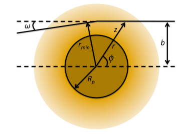
Figure 1: Geometry and parameters relevant to occultation and transit. In occultation, rays enter from the right of the figure, with impact parameter $b$, are bent by atmospheric refraction through an angle $\omega$, and have a distance of closest approach $r_{min}$. In transit, rays follow the opposite trajectory. Note also the planetary radius, $R_{p}$, the radial coordinate, $r$, the corresponding vertical height coordinate, $z=r-R_{p}$, and the polar angle, $\phi$.

To date, the similarities between exoplanet transits and solar or stellar occultations by solar systems worlds have not been exploited as a means of bridging these two research fields. While Earth’s atmospheric transmission has been measured during lunar eclipse and interpreted in terms of exoplanet observations [27, 28], these data only probe a limited range of altitudes ($\sim 10$ km, depending on the solar elevation angle), and require corrections for telluric absorption, solar lines, and the lunar albedo. Furthermore, it is clear that, with regards to exoplanetary science, what is needed is a better understanding of how high altitude hazes influence transmission spectra, and Earth does not have a particularly hazy upper atmosphere.

In this work, we use observations from NASA’s Cassini mission of solar occultations by Titan’s atmosphere to, for the first time ever, produce transit radius spectra of a hazy, well-characterized world. Due to the symmetry in the geometry of occultations and transits, these data inherently include the effects of refraction and aerosol multiple scattering. Our observations provide an essential and much-needed means of validating exoplanet transit models against Solar System data, and can be used to test proposed approaches for deciphering transit spectra. To better understand how Titan’s high altitude haze affects the transit spectra, we develop an analytic model of haze extinction. Finally, we interpret our spectra within the context of exoplanet observations, yielding new insight into the effects of hazes on transit observations.

1 Observations and Data Processing

Figure 1 shows the geometry and relevant variables of occultation and transit, which are analogous to one another. In transit, rays leave the stellar disk at the left of the diagram, are refracted and attenuated, and exit the atmosphere to travel to the observer, who is effectively an infinite distance away. In occultation, rays from the occulted star come from the right of the diagram. For a distant star, these rays are parallel, while for solar occultations rays can be non-parallel, depending on the angular size of the Sun. These rays are attenuated and refracted by the atmosphere before exiting in the direction of the observer (a relatively short distance $D$ away). Thus, occultation measurements can be readily converted into transit radius spectra.

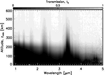
Figure 2: Wavelength dependent transmission through Titan’s atmosphere from the 27^∘ N occultation. The vertical axis is the ray’s altitude of closest approach, where an altitude of zero corresponds to the planetary surface, at a radius of $R_{p}=2575$ km. Darker shades indicate lower transmission, and noise can be seen at transmission values very near to 1 and at wavelengths beyond about 4.5 $\mu$m.

1.1 Occultation Spectra

The Visual and Infrared Mapping Spectrometer (VIMS) [29] aboard NASA’s Cassini orbiter has observed ten solar occultations through Titan’s atmosphere since the beginning of the mission. Spectra are acquired through a special solar port, which attenuates the intensity of sunlight on the detector, span 0.88–5 $\mu$m, and have a spectral resolution between 12–18 nm, increasing with wavelength. Due to technical problems related to pointing stability and parasitic light, only four occultations out of ten could be analyzed. Table 1 summarizes the main parameters of the four datasets.

Table 1. Parameters for Titan Solar Occultation Measurements
Cassini $D$ Resolution Date flyby Season Latitude [km] [km] Jan. 2006 T10 N winter 70^∘ S 8300 15 Apr. 2009 T53 equinox 1^∘ N 6300 7 Sep. 2011 T78 N spring 40^∘ N 9700 10 Sep. 2011 T78 N spring 27^∘ N 8400 10

The atmospheric transmission, $t_{\lambda}$ along the line-of-sight is obtained by taking the ratio of every spectrum to the average spectrum outside the atmosphere (i.e., the reference solar spectrum). This is a self-calibrating method—instrumental effects and systematic errors are removed with the ratio, provided that the occultation is stable and the intensity variations are only due to the atmosphere. Figure 2 shows the altitude-dependent transmission spectra for the 27^∘ N occultation.

The uncertainty on the transmission values are given by the standard deviation over the average of the solar spectrum outside the atmosphere, which is stable except for random noise. Additional details on the data treatment process are described in Maltagliati et al. [30]. We note that these results are in good agreement with the analysis of the 70^∘ S occultation dataset by Bellucci et al. [22], who employed different data processing methods.

Note that the angular diameter of the Sun at Saturn’s orbital distance, $\theta_{\odot}$, is about 1 mrad, so that its image actually subtends a range of altitudes given by $\theta_{\odot}D$, or about 6–10 km. Thus, each individual transmission spectrum contains information from a small range of altitudes. Fortunately this range is smaller than both the vertical resolution of the corresponding datasets (shown in Table 1) and the atmospheric scale height ($\sim 40$ km, implying that atmospheric properties should not change dramatically over the 6–10 km range). Nevertheless, future applications of the techniques described here may need to account for this “smearing” effect, possibly by performing an analysis using a resolved portion of the solar disk (where, then, the relevant angular size is determined by the pixel or instrument field-of-view; see, e.g., [31, 32]).

1.2 Refraction Effects

Refraction has two key effects on occultation observations. The first, and most familiar, is the bending of a light ray as it passes through the atmosphere. This effect is characterized by the refraction angle, $\omega$, which is the angle between the original ray path and the exit path. Generally, the refraction angle is a function of wavelength (due to the wavelength dependent index of refraction of the atmosphere), and causes a distinction between a ray’s impact parameter, $b$, and its distance of closest approach to the planet, $r_{min}$. These parameters are all shown in Figure 1. Refraction is most pronounced for rays that pass near the surface, where molecular number densities are large. Note, however, that, for Titan, strong attenuation by atmospheric haze particles at visible and near-infrared wavelengths largely limits sensitivity to the deep portions of the atmosphere where refractive bending of light rays is most significant.

The second key refractive effect is an apparent brightness loss, which is present even in the absence of molecular and aerosol attenuation [24, 26]. This loss can be thought of as an apparent shrinking of the solar/stellar disk in the vertical direction or, equivalently, a spreading of rays from the source [33]. Here, brightness is diminished by a wavelength dependent factor $f_{\text{ref}}$, which is given by

$$f_{\text{ref}}=\frac{1}{1+Dd\omega/dr_{\text{min}}}\ .$$ (1)

To model these two effects, we use a ray tracing scheme described by van der Werf [34], which concisely outlines an accurate, fourth-order Runge-Kutta integration algorithm for tracking rays through an atmosphere. The primary inputs to this model are profiles of atmospheric density and composition, as well as the refractive indexes of the major atmospheric constituents (which are, generally, wavelength dependent). For Titan, we elect to use standard model profiles of atmospheric molecular number density and composition [35], as localized structure in measured profiles can lead to spurious features in our refraction calculations. Our refraction models only include molecular nitrogen and methane in our computations, as these are the only major atmospheric constituents. Finally, we use a measured, wavelength dependent refractivity for molecular nitrogen [36] and a refractive index for methane of $1.0004478$ [37], although our calculations are largely insensitive to this value due to the low mixing ratio of methane in the atmosphere.

By tracing rays on a fine grid of impact parameters (1 km vertical resolution from 0–1500 km), we determine the relations between the impact parameter, altitudes of closest approach ($z_{\text{min}}=r_{\text{min}}-R_{p}$), refraction angle, and the refractive loss factor $f_{\text{ref}}$. Our computed values are only weak functions of wavelength, as the refractivity of molecular nitrogen changes by less than 1% over the wavelength range of interest. Figure 3 shows profiles of these parameters as a function of their altitude of closest approach, and demonstrates that, for our purposes, refraction effects are only important in the lowest 100 km of the atmosphere.

Figure 3: Profiles of the impact parameter, $b$, refraction angle, $\omega$, and the refractive loss factor, $f_{\text{ref}}$, from our Titan ray tracing model. The vertical coordinate is the ray’s altitude of closest approach, $z_{\text{min}}$. Parameters are shown for a wavelength of 5 $\mu$m, where Titan’s atmospheric haze is least opaque, and we use a distance, $D$, from the spacecraft to Titan of 8400 km, appropriate for the 27^∘ N occultation, when computing the refractive loss. The dotted line plots along the diagonal, and shows that the impact parameter is always larger than the distance of closest approach.

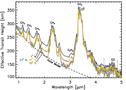
Figure 4: Spectra of effective transit height, $z_{\text{eff},\lambda}=R_{\text{eff},\lambda}-R_{p}$, for all four Cassini/VIMS occultation datasets. Key absorption features are labeled, and error bars are shown only where the 1-$\sigma$ uncertainty is larger than 1%. Our best-fit haze model for the 70^∘S dataset is shown (dashed line).

We note that refraction can also influence exoplanet transit observations under conditions where atmospheric opacity does not preclude light rays from reaching the deeper regions of an atmosphere. Here, the finite size of the host star paired with the geometry of refraction may prevent rays from probing altitudes below some critical height in the lower atmosphere [38]. Additionally, the transit signal may increase or decrease slightly due to the competing effects of refraction bending rays perpendicular to the limb while also focusing rays from within the planet’s shadow towards the observer [39, 40, 41].

1.3 Computing Transit Spectra

We define the transmission corrected for refractive losses at an impact parameter $b_{i}$ as $t^{\prime}_{\lambda,i}=t_{\lambda,i}/f_{\text{ref},i}$ (where a subscript ‘$i$’ references the vertical gridding of the observed transmission spectra). These can be converted into a transit radius spectrum by considering the attenuation produced by concentric annuli above Titan’s surface. An annulus has thickness $\pi\left(b_{i+1}^{2}-b_{i}^{2}\right)$, and we can define an effective transit radius as [42]

$$R_{\text{eff},\lambda}^{2}=R_{\text{top}}^{2}-\sum_{i=1}^{N}\left(\frac{t^{\prime}_{\lambda,i+1}+t^{\prime}_{\lambda,i}}{2}\right)\left(b_{\lambda,i+1}^{2}-b_{\lambda,i}^{2}\right)\ ,$$ (2)

where $R_{\text{top}}=R_{p}+z_{\text{atm}}$ is the radial distance to the top of the atmosphere, whose altitude ($z_{\text{atm}}$) is large enough that atmospheric extinction and refraction are assumed to be negligible. We also define an effective transit height as $z_{\text{eff},\lambda}=R_{\text{eff},\lambda}-R_{p}$, which is useful for identifying where in the atmosphere a given wavelength is probing. Finally, note that the transit depth is proportional to $R_{\text{eff},\lambda}^{2}$, or, equivalently, $\left(z_{\text{eff},\lambda}+R_{p}\right)^{2}$.

2 Transit Radius Spectra

Figure 4 shows the effective transit height, $z_{\text{eff},\lambda}$, for all four occultation datasets. Error bars (1-$\sigma$) are shown where the errors are larger than 1% of the transit height, and key absorption features are identified. In general, errors tend to be large beyond about 4 $\mu$m, where the solar flux is relatively weak.

The most obvious features are the methane bands at 1.2, 1.4, 1.7, 2.3, and 3.3 $\mu$m. Weak absorption due to acetylene (C₂H₂) can be seen near 3.1 $\mu$m. The 3.3 $\mu$m methane band is blended with other features, including the C-H stretching mode of aliphatic hydrocarbon chains appears near 3.4 $\mu$m [22, 30]. An absorption feature of carbon monoxide, which forms from oxygen ions that precipitate into Titan’s upper atmosphere and react with hydrocarbon species [43], appears near 4.6 $\mu$m, although data are particularly noisy here. Finally, additional absorption has been noted in the 2.3 and 3.3 $\mu$m methane bands [22, 30], which is due to other yet unknown species.

What is possibly the most interesting aspect of these spectra is the wavelength dependent slope of the continuum between the methane bands. When observed across the full wavelength range, this slope produces a transit height variation that is comparable to, or larger than, the gaseous absorption features. Assuming that the continuum is set by haze extinction, which shall be argued later, then the differences between the continuum levels for the four different datasets are related to different haze distributions (both vertically and in particle size) at the different latitudes/times of observation. This is consistent with Titan’s known hemispherical asymmetry [44], which may be caused by seasonally-varying atmospheric circulation patterns [45]. Note that methane clouds in Titan’s atmosphere are found below about 30 km altitude [46], and do not affect our transit spectra, which probe much higher altitudes.

Finally, Figure 5 shows an “average” transit spectrum for Titan, in effective transit height and, as an example, in the transit depth signal for Titan crossing the solar disk. To obtain this result, we performed a weighted average of the four individual spectra in Figure 4. The weights were determined from the latitude distribution of the individual spectra, assuming that the 70^∘S spectrum is representative of latitudes between the south pole and midway to the 1^∘N spectrum, that the 1^∘N spectrum is representative of latitudes midway between the 70^∘S spectrum and the 27^∘N spectrum, and so on. Using these weights, we combine the spectra in $R_{\text{eff},\lambda}^{2}$, which is proportional to the transit depth signal. While this weighted averaging is somewhat crude, as it ignores variations in longitude and time, the goal is only to produce a characteristic spectrum.

Standard deviations computed by comparing our characteristic spectrum to the individual spectra are shown as a shaded swath in Figure 5. The deviations are small near the peaks of methane bands, which probe higher in the atmosphere and are less sensitive to variations in the haze continuum levels. At wavelengths dominated by haze opacity, though, the deviation is much larger. Clearly future occultation measurements could help to better understand latitudinal and seasonal effects on our transit spectra, thus improving our characteristic spectrum.

3 A Simple Haze Extinction Model

To investigate the source and behavior of the continuum in our transit height spectra, we derived an analytic model of extinction by an opacity source that is distributed vertically in the atmosphere with scale height $H_{a}$, and whose absorption cross section, $\sigma_{\lambda}$ varies according to a power law in wavelength, with $\sigma_{\lambda}\propto\lambda^{\beta}$. Ignoring refraction effects, which are negligible at most altitudes probed by our spectra, the wavelength dependent optical depth through the atmosphere for a given impact parameter is (see Appendix)

$$\tau_{\lambda}=2\tau_{0}\left(\frac{\lambda}{\lambda_{0}}\right)^{\beta}\frac{b}{H_{a}}K_{1}\!\!\left(\frac{b}{H_{a}}\right)e^{(R_{p}+z_{0})/H_{a}},$$ (3)

where $\tau_{0}$ is a reference optical depth at altitude $z_{0}$, and $K_{n}(x)$ is a modified Bessel function of the second kind. With this model, a transit spectrum can be generated by finding the value of the impact parameter where $\tau_{\lambda}\approx 1$, which requires solving a transcendental expression.

We fit our analytic model to the continua in the 70^∘S spectrum (selected since this dataset has been previously analyzed), and in the characteristic spectrum, which are shown in Figures 4 and 5, respectively. The free parameters in this fit are the haze scale height, $H_{a}$, the reference optical depth, $\tau_{0}$, and the exponent in the cross section power law, $\beta$. For the 70^∘S dataset, we find $H_{a}=58\pm 7$ km, $\tau_{0}=0.9\pm 0.2$ (at $\lambda_{0}$=0.5 $\mu$m and $z_{0}=$200 km, which we will use hereafter), and $\beta=-2.2\pm 0.2$. For the characteristic spectrum, we find $H_{a}=55\pm 8$ km, $\tau_{0}=0.8\pm 0.4$, and $\beta=-1.9\pm 0.2$. Note that the slope of our power law is not due to pure Rayleigh scattering, which would have $\beta=-4$. Instead it is due to the complexities of haze particle scattering between the limits of pure Rayleigh scattering and geometric optics.

Our parameters are in excellent agreement with in situ measurements reported by Tomasko et al. [47], who found $H_{a}=65$ km (with an uncertainty of 20 km), $\tau_{0}=0.76$, and $\beta=-2.33$ above 80 km altitude . For further comparison, Bellucci et al. [22], in their analysis of the 70^∘S occultation, found $H_{a}=$55–79 km, $\beta=-$1.7–2.2 between 120–300 km altitude, and $\tau_{0}\sim 0.6$. Finally, Hubbard et al. [48], in their analysis of stellar occultations by Titan’s atmosphere, found $\beta=-1.7\pm 0.2$. These comparisons strongly support our conclusion that the continuum level in our transit spectra is set by Titan’s high altitude haze.

4 Implications

The transit spectra shown in Figures 4 and 5 demonstrate that high altitude hazes could have complex and important effects on exoplanet observations. Note that our data span wavelengths that are nearly identical to (or larger than) the spectral coverage of the Near InfraRed Camera (NIRCam), Near InfraRed Spectrograph (NIRSpec), and the Near InfraRed Imager and Slitless Spectrograph (NIRISS) instruments that will launch aboard NASA’s James Webb Space Telescope. Thus, the spectra presented here indicate the types of haze effects that this mission may observe for transiting exoplanets.

For Titan, the haze continuum slope is strongly wavelength dependent, and is certainly not flat. This is contrary to what is commonly assumed in simple transit spectra models. Clearly this continuum slope is of first order importance, as the magnitude of the transit height variations caused by the haze continuum is just as large as the observed gaseous absorption features.

Our transit spectra also show that haze opacity obscures information from the deep atmosphere, limiting the pressures probed to above $\sim 0.1$ mbar at the shortest wavelengths, and $\sim 10$ mbar at the longest wavelengths. Even at the longest wavelengths, the altitudes probed are still 2–3 pressure scale heights above the surface. Furthermore, at most continuum wavelengths in our spectra, haze limits sensitivity to pressures lower than (i.e., altitudes above) the $\sim 1$ mbar level, with this effect becoming more severe at shorter wavelengths. Thus, it is empirically possible for high altitude hazes to strongly limit the planetary characteristics that can be inferred from transit spectra, despite what others have claimed [49]. To further clarify this issue, it would be a very useful exercise to challenge current exoplanet retrieval models [50, 51, 52, 53] with our Titan transit spectra, with the goal of improving our ability to understand and interpret transit observations of hazy exoplanets.

Looking to wavelengths beyond those analyzed here, we note that haze opacity effects in transit will become negligible in the mid-infrared, where refraction and gas absorption will then play a key role in limiting sensitivity to the lower atmosphere. However, haze extinction will have much more dramatic effects at ultraviolet and visible wavelengths, where Titan’s haze particles are strongly absorbing [47]. This will make Rayleigh scattering effects undetectable—a ray passing through the atmosphere with a tangent height of $\sim 300$ km (which is optimistic, as this is appropriate for the shortest wavelengths discussed here, not ultraviolet/visible wavelengths) will encounter $10^{20}$ molecules cm^-2, which isn’t optically thick to Rayleigh scattering by molecular nitrogen except at extreme ultraviolet wavelengths ($\sim 40$ nm) and shorter. Thus, Rayleigh scattering slopes in transit spectra, which have been proposed for constraining partial pressures due to spectrally inactive gases [52], may not be accessible in hazy atmospheres.

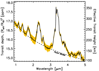
Figure 5: Characteristic transit spectrum for Titan showing both the signal for Titan transiting the Sun (left y-axis) and the effective transit height (right y-axis), assembled as a weighted mean of the four spectra in Figure 4. The shaded region indicates uncertainty in our averaging, and is due to deviations from the mean in the four individual transit spectra. A best-fit haze model is shown (dashed).

Recently, the 6 Earth mass transiting planet GJ 1214b [54] has been the target of many observational campaigns to characterize the nature of its atmosphere [5, 55, 56]. This is the smallest planet with transit spectra observations, which appear to be flat at the 30 ppm level from 1.1–1.7 $\mu$m [57], and this trend may extend to 5 $\mu$m [58]. A Titan-like haze has been proposed as a viable explanation for these observations [17, 18, 19], and the data constrain this haze to be above the $10^{-1}$–$10^{-2}$ mbar level, depending on atmospheric composition [57]. While the methane concentration in the atmosphere of GJ 1214b is unknown, the high altitude haze interpretation isn’t entirely consistent with the observations presented here. Extending Titan’s haze to the aforementioned low pressures would mask the methane features, but still would not produce a flat spectrum due to the wavelength-dependent haze opacity. Thus, a Titan-like haze on GJ 1214b would need to contain a continuum of effective particle radii that extends to sizes larger than is seen for Titan (whose haze particles have a characteristic size of about 1–2 $\mu$m [47], and are aggregates of smaller-sized monomers), as larger particles would tend to produce a flatter spectrum. However, these larger-sized particles may be rather difficult to keep aloft at such low pressures [59], especially given that the gravitational acceleration for GJ 1214b is nearly an order of magnitude larger than that in Titan’s upper atmosphere.

5 Conclusions

We developed a technique for adapting occultation measurements of solar system worlds into transit radius spectra suitable for model validation and comparison to exoplanet observations. We applied this technique to Titan, deriving realistic spectra that inherently include effects due to gas absorption, refraction, and haze scattering, and used these spectra to better understand the effects of high altitude hazes on transit observations. Absorption features due to methane are clearly visible, and weaker features due to acetylene, carbon monoxide, and a C-H stretching mode of aliphatic hydrocarbon chains.

The continuum level in our spectra is set by Titan’s extensive haze, and is well reproduced by an analytic haze extinction model derived here. Haze has a dramatic effect on the transit spectra, limiting sensitivity to pressures smaller than 0.1–10 mbar, depending on wavelength. Extinction from the haze imparts a distinct slope on the transit radius spectra, whose magnitude is comparable to that of the strongest gaseous absorption bands. Thus, haze substantially impacts the amount of information that can be gleaned from transit spectra.

We note that the techniques used here apply equally well to occultation observations taken from orbit around any world. Thus, there are opportunities empirically study the tenuous, dusty atmosphere of Mars [32] and the atmosphere of Saturn [60] in the context of exoplanet transit spectroscopy. Of course, numerous occultation observations exist for Earth [31], which could be used to derive a transit spectrum of the only known habitable planet. Finally, our understanding of how hazes influence transit spectra of Titan could be greatly improved by acquiring additional occultation observations in a Cassini extended mission.

Given the extinction coefficient, $\alpha_{\lambda}=n_{a}\sigma_{\lambda}$, where $n_{a}$ is the absorber number density and $\sigma_{\lambda}$ is the wavelength dependent absorption cross section, the optical depth is determined by the integral

$$\tau_{\lambda}=\int n_{a}\sigma_{\lambda}ds,$$ (4)

where integration proceeds along a ray’s path shown in Figure 1. Ignoring refraction, we have $ds=\left(R_{p}+z\right)d\phi/\sin(\phi)$ and $R_{p}+z=b/\sin(\phi)$, so that

$$\tau_{\lambda}=2\int_{0}^{\pi/2}\frac{b}{\sin^{2}(\phi)}n_{a}\sigma_{\lambda}d\phi,$$ (5)

where we have exploited the symmetry about $\phi=\pi/2$. If the absorber is distributed with a scale height $H_{a}$, with $n_{a}=n_{a0}\exp[-(z-z_{0})/H_{a}]$, where $n_{a0}$ is the number density at the altitude $z_{0}$, and assuming that the absorption cross section is a power law in wavelength, $\sigma_{\lambda}=\sigma_{\lambda 0}\left(\lambda/\lambda_{0}\right)^{\beta}$, where $\lambda$ is wavelength, $\sigma_{\lambda 0}$ is the fiducial value at $\lambda_{0}$, and $\beta$ defines the slope of the power law, we then have

$$\tau_{\lambda}=2\tau_{0}\left(\frac{\lambda}{\lambda_{0}}\right)^{\beta}\frac{b}{H_{a}}e^{\frac{R_{p}+z_{0}}{H_{a}}}\int_{0}^{\pi/2}\frac{e^{-b/H_{a}\sin{\phi}}}{\sin^{2}(\phi)}d\phi,$$ (6)

where $\tau_{0}=n_{a0}\sigma_{\lambda 0}H_{a}$ is a reference vertical optical depth. Making the substitution $\cosh(y)=1/\sin(\phi)$, we have

$$\tau_{\lambda}=2\tau_{0}\left(\frac{\lambda}{\lambda_{0}}\right)^{\beta}\frac{b}{H_{a}}e^{\frac{R_{p}+z_{0}}{H_{a}}}\int_{0}^{\infty}\cosh(y)e^{-\frac{b\cosh(y)}{H_{a}}}dy,$$ (7)

which has the analytic solution given in the main text (Equation 3). Note that, for large $b/H_{a}$, we have $K_{1}(b/H_{a})\sim\sqrt{\pi/2}\exp(-b/H_{a})/\sqrt{b/H_{a}}$, so that Equation 3 gives

$$\tau_{\lambda}\sim\tau_{0}\left(\frac{\lambda}{\lambda_{0}}\right)^{\beta}\sqrt{\frac{2\pi b}{H_{a}}}e^{-(b-R_{p}-z_{0})/H_{a}},$$ (8)

which is in agreement with Fortney [9].

- [1] Sánchez-Lavega A, Pérez-Hoyos S, Hueso R (2004) Clouds in planetary atmospheres: A useful application of the clausius–clapeyron equation. Am J of Phys 72:767–774.
- [2] Pont F, Knutson H, Gilliland R, Moutou C, Charbonneau D (2008) Detection of atmospheric haze on an extrasolar planet: the 0.55–1.05 m transmission spectrum of hd 189733b with the hubble space telescope. Mon Not R Astron Soc 385:109–118.
- [3] Lecavelier Des Etangs A, Pont F, Vidal-Madjar A, Sing D (2008) Rayleigh scattering in the transit spectrum of hd 189733b. Astron Astrophys 481:L83–L86.
- [4] Sing D, et al. (2009) Transit spectrophotometry of the exoplanet hd 189733b. i. searching for water but finding haze with hst nicmos. Astron Astrophys 505:891–899.
- [5] Bean JL, Kempton EMR, Homeier D (2010) A ground-based transmission spectrum of the super-earth exoplanet gj 1214b. Nature 468:669–672.
- [6] Gibson NP, Pont F, Aigrain S (2011) A new look at nicmos transmission spectroscopy of hd 189733, gj-436 and xo-1: no conclusive evidence for molecular features. Mon Not R Astron Soc 411:2199–2213.
- [7] Seager S, Sasselov D (2000) Theoretical transmission spectra during extrasolar giant planet transits. Astrophys J 537:916.
- [8] Charbonneau D, Brown TM, Noyes RW, Gilliland RL (2002) Detection of an Extrasolar Planet Atmosphere. Astrophys J 568:377–384.
- [9] Fortney JJ (2005) The effect of condensates on the characterization of transiting planet atmospheres with transmission spectroscopy. Mon Not R Astron Soc 364:649–653.
- [10] Brown TM (2001) Transmission spectra as diagnostics of extrasolar giant planet atmospheres. Astrophys J 553:1006.
- [11] Hubbard W, et al. (2001) Theory of extrasolar giant planet transits. Astrophys J 560:413.
- [12] Fortney J, et al. (2003) On the indirect detection of sodium in the atmosphere of the planetary companion to hd 209458. Astrophys J 589:615.
- [13] Barman T (2007) Identification of absorption features in an extrasolar planet atmosphere. Astrophys J Lett 661:L191.
- [14] Miller-Ricci E, Seager S, Sasselov D (2009) The Atmospheric Signatures of Super-Earths: How to Distinguish Between Hydrogen-Rich and Hydrogen-Poor Atmospheres. Astrophys J 690:1056–1067.
- [15] Kaltenegger L, Traub W (2009) Transits of earth-like planets. Astrophys J 698:519.
- [16] De Kok R, Stam D (2012) The influence of forward-scattered light in transmission measurements of (exo) planetary atmospheres. Icarus 221:517–524.
- [17] Kempton EMR, Zahnle K, Fortney JJ (2012) The atmospheric chemistry of gj 1214b: photochemistry and clouds. Astrophys J 745:3.
- [18] Howe AR, Burrows AS (2012) Theoretical transit spectra for gj 1214b and other. Astrophys J 756:176.
- [19] Morley CV, et al. (2013) Quantitatively assessing the role of clouds in the transmission spectrum of gj 1214b. Astrophys J 775:33.
- [20] Lunine JI (2010) Titan and habitable planets around m-dwarfs. Faraday discuss 147:405–418.
- [21] Porco CC, et al. (2005) Imaging of titan from the cassini spacecraft. Nature 434:159–168.
- [22] Bellucci A, et al. (2009) Titan solar occultation observed by cassini/vims: Gas absorption and constraints on aerosol composition. Icarus 201:198–216.
- [23] Brown RH, Lebreton JP, Waite JH (2009) Titan from Cassini-Huygens (Springer).
- [24] Elliot J, Olkin C (1996) Probing planetary atmospheres with stellar occultations. Annu Rev Earth Planet Sci 24:89–123.
- [25] Broadfoot A, et al. (1979) Extreme ultraviolet observations from voyager 1 encounter with jupiter. Science 204:979–982.
- [26] Hubbard W, Hunten D, Dieters S, Hill K, Watson R (1988) Occultation evidence for an atmosphere on pluto. Nature 336:452–454.
- [27] Pallé E, Osorio MRZ, Barrena R, Montañés-Rodríguez P, Martín EL (2009) Earth’s transmission spectrum from lunar eclipse observations. Nature 459:814–816.
- [28] Vidal-Madjar A, et al. (2010) The earth as an extrasolar transiting planet. earth’s atmospheric composition and thickness revealed by lunar eclipse observations. Astron Astrophys 523:57.
- [29] Brown R, et al. (2004) in The Cassini-Huygens Mission (Springer), pp 111–168.
- [30] Maltagliati L, et al. (2014) Titan’s atmosphere as observed by VIMS/Cassini solar occultations: CH4, CO and evidence for C2H6 absorption. arXiv:1405.6324.
- [31] Gunson MR, et al. (1996) The atmospheric trace molecule spectroscopy (atmos) experiment: Deployment on the atlas space shuttle missions. Geophys Res Lett 23:2333–2336.
- [32] Maltagliati L, et al. (2013) Annual survey of water vapor vertical distribution and water–aerosol coupling in the martian atmosphere observed by spicam/mex solar occultations. Icarus 223:942–962.
- [33] Baum WA, Code AD (1953) A photometric observation of the occultation of ARIETIS by Jupiter. Astron J 58:108–112.
- [34] van der Werf S (2008) Comment on” improved ray tracing air mass numbers model”. Appl Opt 47:153.
- [35] Waite J, Bell J, Lorenz R, Achterberg R, Flasar F (2013) A model of variability in titan’s atmospheric structure. Planet Space Sci 86:45–56.
- [36] Washburn EW (1930) International Critical Tables of Numerical Data: Physics, Chemistry and Technology (McGraw-Hill, New York) Vol. 7.
- [37] Weber M (2002) Handbook of Optical Materials, Laser & Optical Science & Technology (Taylor & Francis).
- [38] Betremieux Y, Kaltenegger L (2013) Impact of atmospheric refraction: How deeply can we probe exo-Earth’s atmospheres during primary eclipse observations? arXiv:1312.6625.
- [39] French RG (1977) On the theory and analysis of occultation light curves. PhD thesis (Cornell University, Ithaca, NY)
- [40] Hubbard WB (1977) Wave optics of the central spot in planetary occultations. Nature 268:34–35
- [41] Hui L, Seager S (2002) Atmospheric lensing and oblateness effects during an extrasolar planetary transit. Astrophys J 572:540.
- [42] Bétrémieux Y, Kaltenegger L (2013) Transmission spectrum of earth as a transiting exoplanet from the ultraviolet to the near-infrared. Astrophys J Lett 772:L31.
- [43] Hörst SM, Vuitton V, Yelle RV (2008) Origin of oxygen species in titan’s atmosphere. J Geophys Res: Planets 113.
- [44] Sromovsky LA, et al. (1981) Implications of titan’s north–south brightness asymmetry. Nature 292:698–702.
- [45] Rannou P, Hourdin F, McKay C (2002) A wind origin for titan’s haze structure. Nature 418:853–856.
- [46] Rannou P, Montmessin F, Hourdin F, Lebonnois S (2006) The latitudinal distribution of clouds on titan. Science 311:201–205.
- [47] Tomasko M, et al. (2008) A model of titan’s aerosols based on measurements made inside the atmosphere. Planet Space Sci 56:669–707.
- [48] Hubbard W, et al. (1993) The occultation of 28 sgr by titan. Astron Astrophys 269:541–563.
- [49] de Wit J, Seager S (2013) Constraining exoplanet mass from transmission spectroscopy. Science 342:1473–1477.
- [50] Madhusudhan N, Seager S (2009) A Temperature and Abundance Retrieval Method for Exoplanet Atmospheres. Astrophys J 707:24–39.
- [51] Lee JM, Fletcher LN, Irwin PGJ (2012) Optimal estimation retrievals of the atmospheric structure and composition of HD 189733b from secondary eclipse spectroscopy. Mon Not R Astron Soc 420:170–182.
- [52] Benneke B, Seager S (2012) Atmospheric retrieval for super-earths: uniquely constraining the atmospheric composition with transmission spectroscopy. Astrophys J 753:100.
- [53] Line MR, et al. (2013) A systematic retrieval analysis of secondary eclipse spectra. i. a comparison of atmospheric retrieval techniques. Astrophys J 775:137.
- [54] Charbonneau D, et al. (2009) A super-Earth transiting a nearby low-mass star. Nature 462:891–894.
- [55] Désert JM, et al. (2011) Observational Evidence for a Metal-rich Atmosphere on the Super-Earth GJ1214b. Astrophys J Lett 731:L40.
- [56] Berta ZK, et al. (2012) The flat transmission spectrum of the super-earth gj1214b from wide field camera 3 on the hubble space telescope. Astrophys J 747:35.
- [57] Kreidberg L, et al. (2014) Clouds in the atmosphere of the super-earth exoplanet gj 1214b. Nature 505:69–72.
- [58] Fraine JD, et al. (2013) Spitzer transits of the super-earth gj1214b and implications for its atmosphere. Astrophys J 765:127.
- [59] Spiegel DS, Silverio K, Burrows A (2009) Can tio explain thermal inversions in the upper atmospheres of irradiated giant planets? Astrophys J 699:1487.
- [60] Banfield D, Gierasch P, Conrath B, Nicholson P, Hedman M (2011) Saturn’s he and ch4 abundances from cassini vims occultations & cirs limb spectra. EPSC-DPS Joint Meeting 2011 p 1548.