Phase transitions in layered systems

Abstract

We consider the Ising model on $\mathbb{Z}\times\mathbb{Z}$ where on each horizontal line $\{(x,i),x\in\mathbb{Z}\}$, called “layer”, the interaction is given by a ferromagnetic Kac potential with coupling strength $J_{\gamma}(x,y)={\gamma}J({\gamma}(x-y))$, where $J(\cdot)$ is smooth and has compact support; we then add a nearest neighbor ferromagnetic vertical interaction of strength ${\gamma}^{A}$, where $A\geq 2$ is fixed, and prove that for any $\beta$ larger than the mean field critical value there is a phase transition for all ${\gamma}$ small enough.

Key words: Kac potentials, phase transitions, Peierls estimates

AMS Classification: 60K35, 82B20

1 Introduction

We consider the Ising model on the lattice $\mathbb{Z}\times\mathbb{Z}$, denoting by $(x,i)$ its points. On each horizontal line $\{(x,i),x\in\mathbb{Z}\}$, called the $i$-th “layer”, the interaction is given by a ferromagnetic Kac potential so that the interaction between the spins at $(x,i)$ and $(y,i)$ is

$$-\frac{1}{2}J_{\gamma}(x,y){\sigma}(x,i){\sigma}(y,i),$$ (1.1)

where $J_{\gamma}(x,y)={\gamma}J({\gamma}(x-y))$, and $J(\cdot)$ is a symmetric smooth probability density on ${\mathbb{R}}$ with compact support. To fix the notation we suppose $J(r)=0$ for $|r|\geq 1$. We denote by $H_{\gamma}^{0}$ the Hamiltonian with only the interactions (1.1) on each layer, so that different layers do not interact with each other.

We fix the inverse temperature $\beta>1$ (recalling that $\beta=1$ is the mean field critical value). Since each layer is independent of the others and one dimensional, the system with Hamiltonian $H_{\gamma}^{0}$ does not have phase transitions while its mean field version (as derived by the Lebowitz-Penrose analysis by taking first the thermodynamic limit and then letting ${\gamma}\to 0$) has a phase transition with infinitely many extremal states, each one determined by fixing on each layer a magnetization $\pm m_{\beta}$, $m_{\beta}>0$ the positive solution of the mean field equation

$$m_{\beta}=\tanh\{\beta m_{\beta}\}.$$ (1.2)

Purpose of this paper is to study what happens if we put a “very small nearest neighbor vertical interaction”

$$-{\epsilon}\;{\sigma}(x,i){\sigma}(x,i+1).$$ (1.3)

We take hereafter ${\epsilon}={\gamma}^{A}$, where $A\geq 2$ is fixed, and call $H_{\gamma}$ the Hamiltonian with both interactions, i.e. the horizontal one, (1.1), and the vertical one, (1.3) with ${\epsilon}={\gamma}^{A}$. The Lebowitz-Penrose limit is the same for $H^{0}_{\gamma}$ and $H_{\gamma}$, i.e. it is not changed by the interaction (1.3). However the behavior of the system when ${\gamma}>0$ is fixed (and suitably small) is completely different. Let ${\Lambda}$ be a square in $\mathbb{R}^{2}$ and $\mu_{{\gamma},{\Lambda}}^{\rm per}$ the Gibbs measure with Hamiltonian $H_{\gamma}$ on ${\Lambda}\cap(\mathbb{Z}\times\mathbb{Z})$ with periodic boundary conditions.

Theorem 1.

Fix $\beta>1$. There exists $\gamma_{0}>0$ (depending on $\beta$), so that for all ${\gamma}\in(0,\gamma_{0})$

$${\rm weak}\lim_{{\Lambda}\to\mathbb{R}^{2}}\mu_{{\gamma},{\Lambda}}^{\rm per}=\frac{1}{2}\Big{(}\mu^{+}_{\gamma}+\mu^{-}_{\gamma}\Big{)}$$ (1.4)

where $\mu^{\pm}_{\gamma}$ is the DLR measure obtained by taking the thermodynamic limit with plus, respectively minus, boundary conditions. Also $\mu^{+}_{\gamma}\neq\mu^{-}_{\gamma}$ for all such ${\gamma}$. Furthermore, the expected values of the spins converge as ${\gamma}\to 0$ to their mean field values:

$$\lim_{{\gamma}\to 0}\mu_{{\gamma}}^{\pm}({\sigma}(x,i))=\pm m_{\beta}.$$ (1.5)

The proof is given in the next sections and it is obtained by establishing the validity of the Peierls bounds for contours which are defined on each layer following the coarse-grained procedure in [9]. The strategy for proving phase transitions in $d\geq 2$ Ising systems with Kac potentials, as in [4, 1, 9], is to prove that for ${\gamma}$ small enough the weight of a contour is well approximated by the corresponding free energy excess of the associated Lebowitz-Penrose functional. This does not work here because, due to the smallness of the vertical interaction (1.3), the Lebowitz-Penrose functional does not penalize phase changes between contiguous layers. The analysis of the interaction among layers is the main original part of the present paper and it is based on the following idea.

The typical configurations for the Hamiltonian $H^{0}_{\gamma}$ are made on each layer by sequences of intervals where the empirical averages of the spins are alternatively close to $m_{\beta}$ and $-m_{\beta}$, the length of such intervals scales as $e^{c{\gamma}^{-1}}$ ($c$ a positive constant), as it was first observed in [3]. If this behavior were to persist after the vertical interaction (1.3) it would make the interaction among intervals of different phase in contiguous layers of the order ${\epsilon}e^{c{\gamma}^{-1}}$; if ${\epsilon}$ is a power of ${\gamma}$, as in Theorem 1, the Gibbs factor would depress such configurations and this is behind our proof of the Peierls bounds for contours which describe a phase change between contiguous layers.

We hope our present results will help attacking the following problems which arise naturally from the above considerations:

• What happens in the thermodynamic limit to the Gibbs measure $\mu_{{\gamma},{\Lambda}}^{+,-}$ defined by putting plus boundary conditions on the layers $i\geq 0$ and minus boundary conditions on the layers $i<0$ ? Is the limit a Dobrushin state, maybe when the layers are $d>1$ dimensional ?

• Does the system still have a phase transition when $\beta=1$ (i.e. the mean field critical value) and the vertical interaction (1.3) has strength ${\epsilon}>0$ independent of ${\gamma}$ but arbitrarily small ?

• Does Theorem 1 extend to the case when on each layer line we have a system of hard rods with attractive Kac pair potentials and a small attractive vertical interaction as in (1.3) ? If the answer is positive this would be an example where the original Kac proposal for the liquid-vapor phase transitions can be carried through.

Comments. The idea of considering a Kac type interaction in each layer combined with a fixed nearest neighbor interaction in the vertical direction is by no means new. The reader is referred to a paper by Kac and Helfand [6] in the early sixties. See also [7]. What seems new to us is the consideration of the multiplicity of Gibbs measures for fixed (and very small) values of this vertical interaction, beyond the Lebowitz-Penrose limit.

2 Contours

Following Chapter 9 in [9] we implement the program outlined in the Introduction by a coarse graining procedure. For any $\ell\in\{2^{n},\;n\in\mathbb{Z}\}$, $i\in\mathbb{Z}$ and $k\in\mathbb{Z}$ we set:

$$C^{\ell,i}_{k\ell}=\Big{\{}(x,i):k\ell\leq x<(k+1)\ell\Big{\}},\;\;\;C^{\ell,i}_{x}=C^{\ell,i}_{k\ell}\;{\rm if}\;(x,i)\in C^{\ell,i}_{k\ell}$$ (2.1)

and call $\mathcal{D}^{\ell,i}=\{C^{\ell,i}_{k\ell},k\in\mathbb{Z}\}$, $\mathcal{D}^{\ell}=\{\mathcal{D}^{\ell,i},i\in\mathbb{Z}\}$.

We shall use three basic parameters, two lengths $\ell_{\pm}$ and an accuracy $\zeta>0$ which all depend on ${\gamma}$:

$$\ell_{\pm}={\gamma}^{-(1\pm\alpha)},\quad\zeta={\gamma}^{a},\qquad 1\gg\alpha\gg a>0\,$$ (2.2)

supposing for notational simplicity that $\ell_{\pm}\in\{2^{n},n\in\mathbb{N}_{+}\}$: this is a restriction on ${\gamma}$ and $\alpha$ which could be removed by taking integer parts in (2.2). We shortly call $\ell_{\pm}$ intervals the intervals which belongs to $\mathcal{D}^{\ell_{\pm}}$.

Define the empirical magnetization on the scale $\ell_{-}$ as

$${\sigma}^{(\ell_{-})}(x,i):=\frac{1}{\ell_{-}}\sum_{y:(y,i)\in C^{\ell_{-},i}_{x}}{\sigma}(y,i).$$ (2.3)

The random variables $\eta(x,i)$, $\theta(x,i)$ and $\Theta(x,i)$ are then defined as follows:

• $\eta(x,i)=\pm 1$ if $\displaystyle{\big{|}{\sigma}^{(\ell_{-})}(x,i)\mp m_{\beta}\big{|}\leq\zeta}$ and $=0$ otherwise.

• $\theta(x,i)=1$, [$=-1$], if $\eta(y,i)=1$, [$=-1]$, for all $(y,i)\in C_{x}^{\ell_{+},i}$ and $=0$ otherwise.

• $\Theta(x,i)=1$, [$=-1$], if $\theta(x,i)=1$, [$=-1$], on $C_{x}^{\ell_{+},i}\cup C_{x^{\prime}}^{\ell_{+},i}\cup C_{x^{\prime\prime}}^{\ell_{+},i}$, where the latter are the $\ell_{+}$ intervals immediately to the right and to the left of $C_{x}^{\ell_{+},i}$ and $=0$ otherwise.

The phase of a site $(x,i)$ is “plus” if $\Theta(x,i)=\Theta(x,i\pm 1)=1$, it is “minus” if $\Theta(x,i)=\Theta(x,i\pm 1)=-1$ and it is “undetermined” otherwise. Thus given a spin configuration ${\sigma}$ we have a plus, a minus and an undetermined region. Calling “connected” $(x,i)$ and $(y,j)$ iff $|x-y|\leq 1$, $|i-j|\leq 1$ it then follows (recalling the definition of $\Theta$) that the plus and minus regions are disconnected from each other by the undetermined region.

We shall restrict in the sequel to spin configurations such that $\Theta=1$ outside of a compact (the case when $\Theta=-1$ can be recovered via spin flip). Given such a ${\sigma}$, we call “contours” the pairs ${\Gamma}=({\rm sp}({\Gamma}),\eta_{\Gamma})$, where ${\rm sp}({\Gamma})$ is a maximal connected component of the undetermined region, called “the spatial support of ${\Gamma}$”, and $\eta_{\Gamma}$ is the restriction of $\eta$ to ${\rm sp}({\Gamma})$, called “the specification of ${\Gamma}$”.

Denote by ${\rm ext}({\Gamma})$ the unbounded maximal connected component of the complement of ${\rm sp}({\Gamma})$ and $\partial_{\rm ext}({\Gamma})$ the union of all $\ell_{+}$ intervals in ${\rm ext}({\Gamma})$ which are connected to ${\rm sp}({\Gamma})$. Then (since ${\rm sp}({\Gamma})$ is bounded and connected) $\partial_{\rm ext}({\Gamma})$ is connected; moreover $\Theta\neq 0$ on $\partial_{\rm ext}({\Gamma})$ (because ${\rm sp}({\Gamma})$ is a maximal connected component of the undetermined region) and hence $\Theta$ is constant and different from 0 on $\partial_{\rm ext}({\Gamma})$ (because the plus and minus regions are disconnected). We shall call “plus” a contour ${\Gamma}$ when $\Theta=1$ on $\partial_{\rm ext}({\Gamma})$ and “minus” otherwise. (See Figure 1 for an illustration of a contour.)

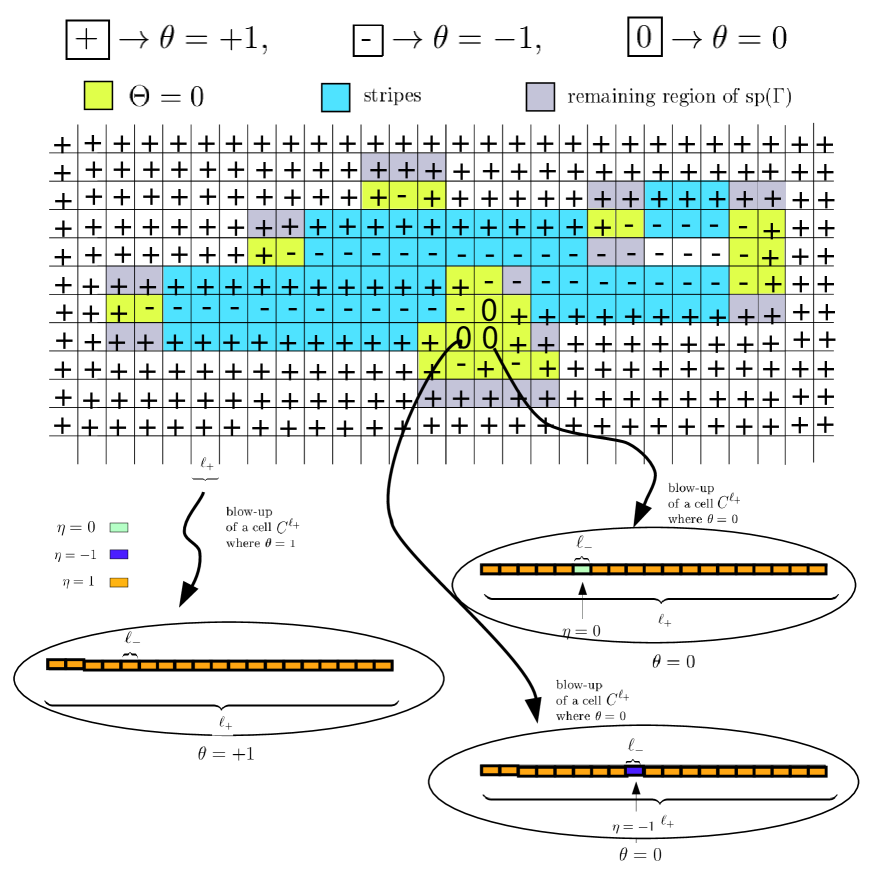
Figure 1: The picture illustrates the support of a contour, marked in the picture by different colors. Each square represents an interval of length $\ell_{+}$ on a line, and the values $+1,0,-1$ correspond to the $\theta$ variables: the color yellow marks the intervals where $\Theta=0$, the light-blue marks intervals where $\Theta$ is $+1$ or $-1$ but in the line below or in the line above the sign is opposite, i.e. the regions denoted as “stripes” . The color grey marks the intervals where $\Theta$ is $+1$ or $-1$ but in the line below or in the line above $\Theta=0$. In the bottom we show some blow-ups of these cells, where $\theta=1$ (the case $\theta=-1$ is similar) and two examples where $\theta=0$.

Analogously we call ${\rm int}_{k}({\Gamma})$ the bounded maximal connected components (if any) of the complement of ${\rm sp}({\Gamma})$, $\partial_{k}({\Gamma})$ the $\ell_{+}$ intervals in ${\rm int}_{k}({\Gamma})$ which are connected to ${\rm sp}({\Gamma})$; then $\Theta$ is constant and different from 0 on each $\partial_{k}({\Gamma})$ and we write $\partial^{\pm}_{k}({\Gamma})$ if $\Theta=\pm 1$. We also call

$$c({\Gamma})={\rm sp}({\Gamma})\cup\bigcup_{k}{\rm int}_{k}({\Gamma}).$$ (2.4)

We are now ready to define the fundamental notion of “weight of a contour”. Let ${\Gamma}$ be a plus contour (the definition for minus contours is obtained by spin flip);

$$\{{\sigma}_{c({\Gamma})}\Rightarrow{\Gamma}\}=\Big{\{}{\sigma}_{c({\Gamma})}:\eta=\eta_{\Gamma}\;{\rm on}\;\,{\rm sp}({\Gamma}),\,\eta_{\Gamma}=\pm 1\;{\rm on\;all}\,\;\partial_{k}^{\pm}({\Gamma})\Big{\}}$$ (2.5)

and $\bar{\sigma}_{\partial_{\rm ext}({\Gamma})}$ a configuration such that $\Theta=1$ on the whole $\partial_{\rm ext}({\Gamma})$. We then define the weight of ${\Gamma}$ with boundary conditions $\bar{\sigma}_{\partial_{\rm ext}({\Gamma})}$ as

$$W_{\Gamma}(\bar{\sigma}_{\partial_{\rm ext}({\Gamma})}):=\frac{Z_{c({\Gamma});\bar{\sigma}_{\partial_{\rm ext}({\Gamma})}}(\{{\sigma}_{c({\Gamma})}\Rightarrow{\Gamma}\})}{Z_{c({\Gamma});\bar{\sigma}_{\partial_{\rm ext}({\Gamma})}}(\{{\sigma}_{c({\Gamma})}:\Theta=1\;\rm{on}\;{\rm sp}({\Gamma})\;{and\;all}\,\partial_{k}^{\pm}({\Gamma})\})},$$ (2.6)

where $Z_{{\Lambda},\bar{\sigma}_{\partial_{\rm ext}({\Lambda})}}(C)$ is the partition function in ${\Lambda}$ with boundary conditions $\bar{\sigma}_{\partial_{\rm ext}({\Lambda})}$ and constraint $C$.

The Peierls argument is based on (a) a bound on the weight of contours and (b) a counting argument for the number of contours which contain a given site. These are established in the next two sections.

3 Energy bounds

We shall prove here bounds on the weight of the contours which are exponentially small with the exponent proportional to the spatial support $|{\rm sp}({\Gamma})|$ of the contour. To this end we introduce the notion of “stripes” in a contour ${\Gamma}$. The spatial support ${\rm sp}(S)$ of a stripe $S$ is a set $\{(x,i):x\in I\}\cup\{(x,i+1):x\in I\}$ where $I=[k\ell_{+},h\ell_{+}-1]$, $k,h\in\mathbb{Z}$, $k<h$. $S$ is a $+-$ stripe in ${\Gamma}$ if ${\rm sp}(S)\subset{\rm sp}({\Gamma})$ and:

• $\Theta=1$ on the upper part of ${\rm sp}(S)$ and $=-1$ on the lower part ($\Theta$ is determined on ${\rm sp}({\Gamma})$ by the specification $\eta_{\Gamma}$ of ${\Gamma}$).

• ${\rm sp}(S)$ is maximal with the above property, namely if $x\in[(k-1)\ell_{+},k\ell_{+})$ then at least one between $\Theta(x,i)$ and $\Theta(x,i+1)$ is equal to 0 and the same holds for $x\in[h\ell_{+},(h+1)\ell_{+})$.

$-+$ stripes are defined analogously (with $-$ on the top). We call $|S|$ the number of sites in the interval $I$ associated to the stripe $S$. We have:

Theorem 2.

There is a positive constant $c$ so that for all ${\gamma}$ small enough the following holds. Let ${\Gamma}$ be any plus contour, $\mathcal{S}$ the set of all stripes in ${\Gamma}$, $|\mathcal{S}|$ the sum of $|S|$ over $S\in\mathcal{S}$ and $N_{0}$ the number of intervals of $\mathcal{D}^{\ell_{+}}$ contained in ${\rm sp}({\Gamma})$ where $\Theta=0$. Then for any $\bar{\sigma}_{\partial_{\rm ext}({\Gamma})}$ such that $\Theta=1$ on $\partial_{\rm ext}({\Gamma})$

$$W_{\Gamma}(\bar{\sigma}_{\partial_{\rm ext}({\Gamma})})\leq e^{-c(N_{0}{\gamma}^{-1+\alpha+2a}+{\gamma}^{A}|\mathcal{S}|)}.$$ (3.1)

Same bound holds for minus contours.

We shall prove Theorem 2 in the rest of the section. Recall that the energy of a spin ${\sigma}(x,i)$ in the field generated by the configuration ${\sigma}^{\prime}$ outside $(x,i)$ is

$$H_{\gamma}({\sigma}(x,i)|{\sigma}^{\prime}):=-{\sigma}(x,i)[h_{\gamma}(x,i;{\sigma}^{\prime})+{\gamma}^{A}({\sigma}(x,i+1)+{\sigma}(x,i-1))]$$

where $h_{\gamma}(x,i;{\sigma}^{\prime}):=\sum_{y\neq x}J_{\gamma}(x,y){\sigma}^{\prime}(y,i)$. Then the Gibbs distribution of ${\sigma}(x,i)$ given ${\sigma}^{\prime}$ is

$$G_{\gamma}({\sigma}(x,i)|{\sigma}^{\prime})=Z_{{\gamma},{\sigma}^{\prime}}^{-1}e^{-\beta H_{\gamma}({\sigma}(x,i)|{\sigma}^{\prime})},$$ (3.2)

with $Z_{{\gamma},{\sigma}^{\prime}}$ the normalization factor. The Gibbs conditional probability of ${\sigma}(x,i)$ given ${\sigma}^{\prime}$ and that $\eta(x,i)=1$, denoted by $\mu({\sigma}(x,i)|{\sigma}^{\prime},\eta(x,i)=1)$, is not always given by (3.2) because the condition $\eta(x,i)=1$ involves the spin ${\sigma}(x,i)$. However we obviously have:

Lemma 1.

Let ${\sigma}^{\prime}$ be such that

$$|\frac{1}{\ell_{-}}\sum_{y\in C^{\ell_{-},i}_{x},y\neq x}{\sigma}^{\prime}(y,i)-m_{\beta}|<\zeta-\frac{1}{\ell_{-}}.$$ (3.3)

Then

$$\mu\Big{(}{\sigma}(x,i)|{\sigma}^{\prime},\eta(x,i)=1\Big{)}=G_{\gamma}({\sigma}(x,i)|{\sigma}^{\prime}).$$ (3.4)

The next lemma gives an upper bound for the probability of violating condition (3.3).

Lemma 2.

There are $b<1$ and $c_{b}>0$ so that for all ${\gamma}$ small enough the following holds. Let ${\sigma}^{\prime}$ be a configuration in the complement of $C^{\ell_{-},i}_{x}$ such that $\eta(y,i)=1$ for all $y$ such that $(y,i)\notin C^{\ell_{-},i}_{x}$. Denote by $\mu(\,\cdot\,|\;{\sigma}^{\prime},\eta(x,i)=1)$ the Gibbs conditional probability on $\{-1,1\}^{C^{\ell_{-},i}_{x}}$ given ${\sigma}^{\prime}$ and that $\eta(x,i)=1$. Then (recalling (2.3) for notation)

$$\mu\Big{(}|{\sigma}^{(\ell_{-})}(x,i)-m_{\beta}|>b\zeta\;|\;{\sigma}^{\prime},\eta(x,i)=1\Big{)}\leq e^{-c_{b}\ell_{-}\zeta^{2}}.$$ (3.5)

Proof.

Since the model is translation invariant, we may take $x=i=0$. Let $\sigma_{y}$ stand for $\sigma(y,0)$, $y\in{\mathbb{Z}}$, and let $\sigma^{\pm}_{y}=\sigma^{\prime}(y,\pm 1)$. We write ${\cal C}_{k}^{\ell_{-}}=C_{k\ell_{-}}^{\ell_{-},0}$, $k\in{\mathbb{Z}}$.

The relevant Hamiltonian is then, for $\sigma=(\sigma_{y})_{y\in{\cal C}_{0}^{\ell_{-}}}$

$$H(\sigma)=H_{c}(\sigma)+H_{b}(\sigma)$$ (3.6)

where

$$H_{c}(\sigma)=-\gamma^{\alpha}\sum_{y\in{\cal C}_{0}^{\ell_{-}}}\sigma_{y}\sigma_{0}^{(\ell_{-},y)},\quad H_{b}(\sigma)=-\sum_{y\in{\cal C}_{0}^{\ell_{-}}}\sigma_{y}h_{y},$$ (3.7)

$$\sigma_{k}^{(\ell_{-},y)}=\frac{1}{\ell_{-}}\sum_{z\in{\cal C}_{k}^{\ell_{-}}}J\left(\gamma(z-y)\right)\sigma_{z},$$ (3.8)

and

$$h_{y}=\gamma^{\alpha}\sum_{k\in{\mathbb{Z}}\atop{k\neq 0}}\sigma_{k}^{(\ell_{-},y)}+\gamma^{A}(\sigma_{y}^{+}+\sigma_{y}^{-}).$$ (3.9)

Given the conditions on the boundary and on $J$, it is a straightforward matter to check that there exists a positive constant $\kappa$ such that for every $y\in{\cal C}_{0}^{\ell_{-}}$

$$|h_{y}-m_{\beta}|\leq\zeta+\kappa\gamma^{\alpha}.$$ (3.10)

The claim of the lemma follows readily from the same bound for the probability of the same event without the conditioning on $\eta(0,0)=1$ (with a possibly different $c_{b}$), so we will verify the latter bound only.

We first dominate in the FKG sense from above and below the model in the volume ${\cal C}_{0}^{\ell_{-}}$ with the given boundary conditions by appropriate models without pair couplings within ${\cal C}_{0}^{\ell_{-}}$, only couplings to the boundary and extra external magnetic fields, so that we will indeed have independent spins in ${\cal C}_{0}^{\ell_{-}}$ subject to a (uniform) external field appropriately close to $m_{\beta}$.

For a given constant $M>0$ to be fixed later, let $\mu^{\pm}$ be the Gibbs measures on spin configurations in ${\cal C}_{0}^{\ell_{-}}$ with the following Hamiltonians.

$$H^{\pm}(\sigma)=-\sum_{y\in{\cal C}_{0}^{\ell_{-}}}\sigma_{y}h^{\pm}_{y},$$ (3.11)

where

$$h^{\pm}_{y}\equiv m_{\beta}\pm[\zeta+(M+\kappa)\gamma^{\alpha}].$$ (3.12)

The result will then follow once we show that

$$\mu^{-}(\cdot)\leq\mu(\cdot|\sigma^{\prime})\leq\mu^{+}(\cdot)$$ (3.13)

(in the FKG sense), where $\mu$ is the Gibbs measure, and that the bound holds for the probabilities

$$\mu^{+}(\sigma^{(\ell_{-})}>m_{\beta}+b\zeta),$$ (3.14)

$$\mu^{-}(\sigma^{(\ell_{-})}<m_{\beta}-b\zeta),$$ (3.15)

for some $b\in(0,1)$, as soon as $\gamma$ is close enough to $0$, where $\sigma^{(\ell_{-})}=\frac{1}{\ell_{-}}\sum_{y\in{\cal C}_{0}^{\ell_{-}}}\sigma_{y}$.

An upper bound of the form (3.5) for the expression in (3.14) follows readily from well-known large deviation bounds, say Bernstein inequality (see e.g. Lemma 1, p. 533 in [8]), once we notice that under $\mu^{+}$, the spins in ${\cal C}_{0}^{\ell_{-}}$ are iid random variables on $\{-1,+1\}$ with mean

$$t_{\beta}(m_{\beta}+\zeta+(M+\kappa)\gamma^{\alpha})\leq m_{\beta}+t_{\beta}^{\prime}(m_{\beta})[\zeta+(M+\kappa)\gamma^{\alpha}]\leq m_{\beta}+\tilde{b}\zeta,$$ (3.16)

where $t_{\beta}:{\mathbb{R}}\to(-1,1)$ is such that $t_{\beta}(x)=\tanh(\beta x)$, and $\tilde{b}<1$ as soon as $\gamma$ is close enough to $0$, since the derivative of $t_{\beta}$ is less than one on $m_{\beta}$ for $\beta>1$. A similar argument establishes a similar bound for the expression in (3.15).

It remains to establish (3.13). We will prove the upper bound. An argument for the lower bound can be made similarly.

Proof of the upper bound in (3.13)

We will verify Holley’s condition (see [5]), which in this case reduces to the following bound. Given $\sigma,\tau\in\{-1,+1\}^{{\cal C}_{0}^{\ell_{-}}}$

$$-H(\sigma\wedge\tau)-H^{+}(\sigma\vee\tau)\geq-H(\sigma)-H^{+}(\tau),$$ (3.17)

which in turn reduces to

$$\sum_{y\in{\cal C}_{0}^{\ell_{-}}}(\sigma\wedge\tau)_{y}\{\gamma^{\alpha}(\sigma\wedge\tau)_{0}^{(\ell_{-},y)}+h_{y}\}+\sum_{y\in{\cal C}_{0}^{\ell_{-}}}(\sigma\vee\tau)_{y}\{M\gamma^{\alpha}+\tilde{h}_{y}\}$$

$$\geq\sum_{y\in{\cal C}_{0}^{\ell_{-}}}\sigma_{y}\{\gamma^{\alpha}\sigma_{0}^{(\ell_{-},y)}+h_{y}\}+\sum_{y\in{\cal C}_{0}^{\ell_{-}}}\tau_{y}\{M\gamma^{\alpha}+\tilde{h}_{y}\},$$ (3.18)

where $\tilde{h}_{y}\equiv m_{\beta}+\zeta+\kappa\gamma^{\alpha}$. We first show that

$$\sum_{y\in{\cal C}_{0}^{\ell_{-}}}(\sigma\wedge\tau)_{y}h_{y}+\sum_{y\in{\cal C}_{0}^{\ell_{-}}}(\sigma\vee\tau)_{y}\tilde{h}_{y}\geq\sum_{y\in{\cal C}_{0}^{\ell_{-}}}\sigma_{y}h_{y}+\sum_{y\in{\cal C}_{0}^{\ell_{-}}}\tau_{y}\tilde{h}_{y},$$ (3.19)

which is equivalent to

$$\sum_{y\in{\cal C}_{0}^{\ell_{-}}}[(\sigma\vee\tau)_{y}-\tau_{y}]\tilde{h}_{y}\geq\sum_{y\in{\cal C}_{0}^{\ell_{-}}}[\sigma_{y}-(\sigma\wedge\tau)_{y}]h_{y}.$$ (3.20)

But $(\sigma\vee\tau)_{y}-\tau_{y}=\sigma_{y}-(\sigma\wedge\tau)_{y}\geq 0$ for all $y$, and (3.20) follows from (3.10), and thence (3.19) holds. It is enough then to show that

$$\sum_{y\in{\cal C}_{0}^{\ell_{-}}}(\sigma\wedge\tau)_{y}(\sigma\wedge\tau)_{0}^{(\ell_{-},y)}+M\sum_{y\in{\cal C}_{0}^{\ell_{-}}}(\sigma\vee\tau)_{y}$$

$$\geq\sum_{y\in{\cal C}_{0}^{\ell_{-}}}\sigma_{y}\sigma_{0}^{(\ell_{-},y)}+M\sum_{y\in{\cal C}_{0}^{\ell_{-}}}\tau_{y},$$ (3.21)

which is equivalent to

$$M\ell_{-}\sum_{y\in{\cal C}_{0}^{\ell_{-}}}[(\sigma\vee\tau)_{y}-\tau_{y}]=M\ell_{-}\sum_{y\in{\cal C}_{0}^{\ell_{-}}}[\sigma_{y}-(\sigma\wedge\tau)_{y}]$$

$$\geq\sum_{y,z\in{\cal C}_{0}^{\ell_{-}}}J\left(\gamma(z-y)\right)[\sigma_{y}\sigma_{z}-(\sigma\wedge\tau)_{y}(\sigma\wedge\tau)_{z}].$$ (3.22)

Let ${\cal L}={\cal L}(\sigma,\tau)=\{x\in{\cal C}_{0}^{\ell_{-}}:\,\sigma_{x}>\tau_{x}\}$, $\tilde{\ell}=|{\cal L}|$, and ${\cal L}^{c}={\cal C}_{0}^{\ell_{-}}\setminus{\cal L}$. Then the expression on the top of (3.22) equals $2M\ell_{-}\tilde{\ell}$ and the one in the bottom equals

$$2\sum_{y\in{\cal L},z\in{\cal L}^{c}}J\left(\gamma(z-y)\right)\sigma_{z}+2\sum_{y\in{\cal L}^{c},z\in{\cal L}}J\left(\gamma(z-y)\right)\sigma_{y}$$

$$\leq 2\sum_{y\in{\cal L},z\in{\cal L}^{c}}J\left(\gamma(z-y)\right)+2\sum_{y\in{\cal L}^{c},z\in{\cal L}}J\left(\gamma(z-y)\right)$$

$$\leq 4\tilde{M}\tilde{\ell}(\ell_{-}-\tilde{\ell})\leq 4\tilde{M}\ell_{-}\tilde{\ell},$$ (3.23)

where $\tilde{M}=\sup_{|r|\leq\gamma^{\alpha}}J(r)$. We conclude that (3.22) holds as soon as

$$M>2J(0)$$ (3.24)

and $\gamma$ is close enough to $0$. Let us then fix an $M$ satisfying (3.24). We may conclude that Holley’s condition is verified for all $\gamma$ close enough to $0$, and thence so is the upper bound in (3.13). ∎

Remarks.

• Recall that the interaction range is ${\gamma}^{-1}$ so that the condition $\eta(y,i)=1$ can be required to hold only in the $\ell_{-}$ intervals on the $i$-th layer which have distance $\leq{\gamma}^{-1}$ from $C^{\ell_{-},i}_{x}$.

• By the spin flip symmetry Lemma 2 extends to the case where $\eta(y,i)=-1$ with $m_{\beta}\to-m_{\beta}$ in (3.5).

• Suppose that (3.3) is violated. Then, for ${\gamma}$ small enough, $|{{\sigma}^{\prime}}^{(\ell_{-})}(x,i)-m_{\beta}|>b\zeta$ no matter what is the value of ${\sigma}^{\prime}(x,i)$.

We can now start the proof of the Peierls bound which will be achieved after several manipulations of the partition function in the numerator of the fraction on the right hand side of (2.6). The first step is to eliminate some of the vertical interactions in ${\rm sp}({\Gamma})$. Let $S$ be a $+-$ stripe, ${\rm sp}(S)=\{(x,j):x\in I,j=i,i+1\}$. Denote by ${\sigma}^{\prime}$ a configuration on the complement of ${\rm sp}(S)$. By the definition of stripes, ${\sigma}^{\prime}$ is such that $\eta=1$ on all the $\ell_{-}$ intervals on the layer $i+1$ which have distance $\leq{\gamma}^{-1}$ from ${\rm sp}(S)$ and $\eta=-1$ on all the $\ell_{-}$ intervals on the layer $i$ which have distance $\leq{\gamma}^{-1}$ from ${\rm sp}(S)$. We shorthand by $Z_{S,{\sigma}^{\prime}}$ the partition function on ${\rm sp}(S)$ with boundary conditions ${\sigma}^{\prime}$ and constraint $\{\eta=\pm 1\}$ on the upper and respectively lower layers of ${\rm sp}(S)$. We denote by $Z^{0}_{S,{\sigma}^{\prime}}$ the same partition function but with the vertical interaction among the upper and lower layers of ${\rm sp}(S)$ removed, the vertical interaction with the complement of ${\rm sp}(S)$ is instead kept.

Proposition 1.

There is $c>0$ so that for all ${\gamma}$ small enough

$$Z_{S,{\sigma}^{\prime}}\leq e^{-c{\gamma}^{A}|S|}\;Z^{0}_{S,{\sigma}^{\prime}}.$$

Proof.

Let $\mu^{\epsilon}_{S,{\sigma}^{\prime}}(\cdot)$ be the Gibbs measure where the vertical interaction in $S$ is ${\epsilon}$ instead of ${\gamma}^{A}$, with $0<{\epsilon}\leq{\gamma}^{A}$. We have:

$$\log\frac{Z_{S,{\sigma}^{\prime}}}{Z^{0}_{S,{\sigma}^{\prime}}}=\sum_{x\in I}\int_{0}^{{\gamma}^{A}}\mu^{\epsilon}_{S,{\sigma}^{\prime}}({\sigma}(x,i){\sigma}(x,i+1))d{\epsilon}.$$ (3.25)

We compute $\mu^{\epsilon}_{S,{\sigma}^{\prime}}({\sigma}(x,i){\sigma}(x,i+1))$ by first conditioning on ${\sigma}^{\prime\prime}$, the configuration restricted to $sp(S)\setminus\{(x,i)(x,i+1)\}$:

$$\mu^{\epsilon}_{S,{\sigma}^{\prime}}({\sigma}(x,i){\sigma}(x,i+1)) = \mu^{\epsilon}_{S,{\sigma}^{\prime}}\left[\mu^{\epsilon}_{S,{\sigma}^{\prime}}({\sigma}(x,i){\sigma}(x,i+1))\mid{\sigma}^{\prime},{\sigma}^{\prime\prime},\eta(x,i)=-1,\eta(x,i+1)=+1\right]$$ (3.26)

$$= \mu^{\epsilon}_{S,{\sigma}^{\prime}}\left[\mathbf{1}_{B_{x}}\mu^{\epsilon}_{S,{\sigma}^{\prime}}({\sigma}(x,i){\sigma}(x,i+1))\mid{\sigma}^{\prime},{\sigma}^{\prime\prime}\right]+O(e^{-c\ell_{-}\zeta^{2}})$$

where:

$$B_{x}:=\left\{{\sigma}^{\prime\prime}:|\frac{1}{\ell_{-}}\sum_{y\in C^{\ell_{-},i}_{x},y\neq x}{\sigma}^{\prime\prime}(y,i)+m_{\beta}|<\zeta-\frac{1}{\ell_{-}};\,|\frac{1}{\ell_{-}}\sum_{y\in C^{\ell_{-},i+1}_{x},y\neq x}{\sigma}^{\prime\prime}(y,i+1)-m_{\beta}|<\zeta-\frac{1}{\ell_{-}}\right\}$$ (3.27)

and we have used that $\mu^{\epsilon}_{S,{\sigma}^{\prime}}(B^{c}_{x})<O(e^{-c\ell_{-}\zeta^{2}})$ uniformly in ${\epsilon}<{\gamma}^{A}$.

It can been seen that on $B_{x}$,

$$|\mu^{\epsilon}_{S,{\sigma}^{\prime}}({\sigma}(x,i){\sigma}(x,i+1)|{\sigma}^{\prime},{\sigma}^{\prime\prime})+m^{2}_{\beta}| = O(\zeta)$$ (3.28)

since the vertical interactions in $x$ are uniformly bounded by ${\gamma}^{A}$.

Summing up in $x\in I$ we conclude the statement

$$\log\frac{Z_{S,{\sigma}^{\prime}}}{Z^{0}_{S,{\sigma}^{\prime}}}\leq-|I|{\gamma}^{A}[m_{\beta}^{2}-O(\zeta)].$$ (3.29)

∎

As an immediate corollary of Proposition 1 we have:

Corollary 1.

Denote by $Z^{0,\mathcal{S}}_{c({\Gamma});\bar{\sigma}_{\partial_{\rm ext}({\Gamma})}}(\{{\sigma}_{c({\Gamma})}\Rightarrow{\Gamma}\})$ the partition function in the numerator of (2.6) with the vertical interaction among the upper and lower layers of all ${\rm sp}(S)$, $S\in\mathcal{S}$, removed. Then for all ${\gamma}$ small enough

$$Z_{c({\Gamma});\bar{\sigma}_{\partial_{\rm ext}({\Gamma})}}(\{{\sigma}_{c({\Gamma})}\Rightarrow{\Gamma}\})\leq e^{-c{\gamma}^{A}|\mathcal{S}|}\;Z^{0,\mathcal{S}}_{c({\Gamma});\bar{\sigma}_{\partial_{\rm ext}({\Gamma})}}(\{{\sigma}_{c({\Gamma})}\Rightarrow{\Gamma}\})$$ (3.30)

with $c$ as in Proposition 1.

Denote by $Z^{0}_{c({\Gamma});\bar{\sigma}_{\partial_{\rm ext}({\Gamma})}}(\{{\sigma}_{c({\Gamma})}\Rightarrow{\Gamma}\})$ the partition function in the numerator of (2.6) where it has been removed the vertical interaction between any two intervals $C^{\ell_{+},i+1}_{x}$ and $C^{\ell_{+},i}_{x}$ both in ${\rm sp}({\Gamma})$ such that either (i) $\Theta$ has opposite sign (i.e. they belong to a stripe) or (ii) $\Theta=0$ at least on one of them.

Corollary 2.

Let $Z^{0}_{c({\Gamma});\bar{\sigma}_{\partial_{\rm ext}({\Gamma})}}(\{{\sigma}_{c({\Gamma})}\Rightarrow{\Gamma}\})$ be as above. Then for all ${\gamma}$ small enough

$$Z_{c({\Gamma});\bar{\sigma}_{\partial_{\rm ext}({\Gamma})}}(\{{\sigma}_{c({\Gamma})}\Rightarrow{\Gamma}\})\leq e^{-c{\gamma}^{A}|\mathcal{S}|+2{\gamma}^{A}\ell_{+}N_{0}}\;Z^{0}_{c({\Gamma});\bar{\sigma}_{\partial_{\rm ext}({\Gamma})}}(\{{\sigma}_{c({\Gamma})}\Rightarrow{\Gamma}\})$$ (3.31)

($c$ as in Proposition 1 and $N_{0}$ the number of $\mathcal{D}^{\ell_{+}}$ intervals in ${\rm sp}({\Gamma})$ where $\Theta=0$).

Call

$$\Delta:=\Big{\{}(x,i)\in{\rm sp}({\Gamma}):\Theta(x,i)=0\Big{\}},\quad|\Delta|=\ell_{+}N_{0}$$ (3.32)

and denote by ${\sigma}_{\Delta}$ and ${\sigma}^{\prime}$ the spin configurations in $\Delta$ and respectively outside $\Delta$. Since we have dropped all vertical interactions involving spins in $\Delta$ the system has only Kac interactions. A lot is known about such systems and most of what follows is in fact taken from the existing literature. We fix ${\sigma}^{\prime}$ outside $\Delta$ and need to bound

$$Z^{0}_{\Delta,{\sigma}^{\prime}}(\eta=\eta_{\Gamma}):=\sum_{{\sigma}_{\Delta}}\mathbf{1}_{\{\eta=\eta_{\Gamma}\;{\rm on}\Delta\}}e^{-\beta H_{\gamma}^{0}({\sigma}_{\Delta}|{\sigma}^{\prime})}.$$ (3.33)

Observe that $Z^{0}_{\Delta,{\sigma}^{\prime}}(\eta=\eta_{\Gamma})$ factorizes into a product of partition functions on each layer so that our next estimates will be one-dimensional.

Next step is to coarse-grain to reduce the bound of (3.33) to a variational problem involving a free energy functional defined on functions $m(r,i)$, $r\in\mathbb{R},i\in\mathbb{Z}$. The scale of the coarse-graining should be chosen to have an error small when compared to the gain term in (3.1): a possible choice that we shall adopt is $\ell={\gamma}^{-1/2}$ (which for simplicity we suppose in $\{2^{n},n\in\mathbb{N}\}$).

As a rule we add a $*$ when we go from the discrete to the continuum, so that $\Delta^{*}$ denotes the union over $(x,i)\in\Delta$ of the unit intervals $\{(r,i):x\leq r<x+1\}$. We then have (see Theorem 4.2.2.2 in [9])

$$\log Z^{0}_{\Delta,{\sigma}^{\prime}}(\eta=\eta_{\Gamma})\leq-\beta\;\inf_{m_{\Delta}\in\mathcal{A}}F_{{\gamma},\Delta^{*}}\left(m_{\Delta}|{{\sigma}^{\prime}}^{({\gamma}^{-1/2})}\right)+\beta c{\gamma}^{1/2}\log{\gamma}^{-1}|\Delta|$$ (3.34)

where $m_{\Delta}\in L^{\infty}(\Delta^{*},[-1,1])$; ${\sigma}^{({\gamma}^{-1/2})}$ is the analogue of ${\sigma}^{(\ell_{-})}$ in (2.3) with $\ell_{-}$ replaced by ${\gamma}^{-1/2}$; $\mathcal{A}$ is the set of functions $m$ so that for any $(x,i)\in\Delta$ the difference

$$|\frac{1}{\ell_{-}}\int_{r^{\prime}}^{r^{\prime}+\ell_{-}}m(r,i)dr\mp m_{\beta}|,\quad r^{\prime}=h\ell_{-}\leq x<(h+1)\ell_{-}$$

is smaller or larger than $\zeta$ according to the value of $\eta_{\Gamma}(x,i)$;
$\displaystyle{F_{{\gamma},\Delta^{*}}\left(m_{\Delta}|m_{{\Delta}^{c}}\right)=F_{{\gamma},\Delta^{*}}(m_{\Delta})-\sum_{i}\int\int\mathbf{1}_{\{(r,i)\in\Delta^{*},(r^{\prime},i)\notin{\Delta^{*}}\}}J_{\gamma}(r,r^{\prime})\,m_{\Delta}(r)m_{{\Delta}^{c}}(r^{\prime})}drdr^{\prime}$,
where

$$F_{{\gamma},\Delta^{*}}(m_{\Delta})=-\frac{1}{2}\sum_{i}\int_{\{(r,i)\in\Delta^{*}\}}\int_{\{(r^{\prime},i)\in\Delta^{*}\}}J_{\gamma}(r,r^{\prime})\,m_{\Delta}(r)m_{\Delta}(r^{\prime})drdr^{\prime}-\frac{1}{\beta}\int_{\Delta^{*}}I(m_{\Delta}(r))dr$$

$$I(m)=-\frac{1-m}{2}\log\,\frac{1-m}{2}-\frac{1+m}{2}\log\,\frac{1+m}{2};$$ (3.35)

finally $c$ in (3.34) is a constant.

Observe that the last term in (3.34) is bounded by $\beta cN_{0}{\gamma}^{-1/2-\alpha}\log{\gamma}^{-1}$, thus the “error” in (3.34) is “small” with respect to the gain term in (3.1) (because $a$ and $\alpha$ are suitably small).

The next step exploits the stability property of the functional in a neighborhood of the stationary profiles identically equal to $m_{\beta}$ (or to $-m_{\beta}$). The intersection of a layer $\{(r,i):r\in\mathbb{R}\}$ with $\Delta^{*}$ (supposing it is non empty) is made of consecutive disconnected intervals

$$I_{h,i}=[(r,i):r^{\prime}_{h}\leq r<r^{\prime\prime}_{h}),\quad r^{\prime}_{h},r^{\prime\prime}_{h}\in\ell_{+}\mathbb{Z},$$

where the extremes of the separating intervals $[r^{\prime\prime}_{h},r^{\prime}_{h+1})$ are either the endpoints of a stripe layer, or the intersection with $\{(r,i):r\in\mathbb{R}\}$ of an interior ${\rm int}_{j}({\Gamma})^{*}$. Thus by construction $\theta(r^{\prime}_{h},i)=\pm 1$ and since $m_{\Delta}\in\mathcal{A}$, for all $k$ such that $[k\ell_{-},(k+1)\ell_{-})\subseteq[r^{\prime}_{h},r^{\prime}_{h}+\ell_{+})$ we have either

$$\Big{|}\frac{1}{\ell_{-}}\int_{k\ell_{-}}^{(k+1)\ell_{-}}m_{\Delta}(r)dr-m_{\beta}\Big{|}\leq\zeta$$

or the same with $m_{\beta}\to-m_{\beta}$. The analogous property holds in $[r^{\prime\prime}_{h}-\ell_{+},r^{\prime\prime}_{h})$. Let us focus for instance on the interval $[r^{\prime}_{h},r^{\prime}_{h}+\ell_{+})$, call $r_{{\rm mid}}:=r^{\prime}_{h}+\ell_{+}/2$ and, to fix the ideas, suppose the averages of $m_{\Delta}$ are close to $m_{\beta}$. Then by Theorem 6.3.3.1 in [9] there are ${\omega}>0$ and $c$ so that the inf in (3.34) is achieved on functions $m$ with the following property.

$$\sup_{|r-r_{{\rm mid}}|\leq{\gamma}^{-1}}|m(r)-m_{\beta}|\leq ce^{-{{\omega}}{\gamma}\ell_{+}}=ce^{-{{\omega}}{\gamma}^{-\alpha}}.$$ (3.36)

Thus,

$$\displaystyle{\inf_{m_{\Delta}\in\mathcal{A}}F_{{\gamma},\Delta^{*}}\left(m_{\Delta}|{{\sigma}^{\prime}}^{({\gamma}^{-1/2})}\right)}\geq \inf_{m_{\Delta}\in\mathcal{A};m_{\Delta}=m_{\beta}\;{\rm on}\;|r-r_{{\rm mid}}|\leq{\gamma}^{-1}}F_{{\gamma},\Delta^{*}}\left(m_{\Delta}|{{\sigma}^{\prime}}^{({\gamma}^{-1/2})}\right)$$

$$- {\gamma}^{-1}c^{\prime}e^{-{{\omega}}{\gamma}^{-\alpha}}.$$

By changing the constant $c$ in (3.34) we can then restrict in (3.34) to functions which are identically equal to $m_{\beta}$ or to $-m_{\beta}$ depending on the value of $\eta_{\Gamma}$ in all the intervals of the form $|r-r_{\rm mid}|\leq{\gamma}^{-1}$ with $r_{\rm mid}$ at distance $\ell_{+}/2$ from an endpoint of any of the $I_{h,i}$.

Call $I_{1}=[r^{\prime}_{h},r^{\prime}_{h}+\frac{\ell_{+}}{2}]$, $I_{2}=[r^{\prime\prime}_{h}-\frac{\ell_{+}}{2},r^{\prime\prime}_{h}]$ and $I_{0}=I_{h,i}\setminus\{I_{1}\cup I_{2}\}$. Let $m$ be a function on $I_{h,i}$ equal to $\pm m_{\beta}$ in the two intervals $|r-r_{\rm mid}|\leq{\gamma}^{-1}$, with $r_{\rm mid}$ at distance $\ell_{+}/2$ from $r^{\prime}_{h}$ and from $r^{\prime\prime}_{h}$, respectively. Call $m_{1}$, $m_{2}$ and $m_{0}$ the restriction of $m$ to $I_{1}$, $I_{2}$ and $I_{0}$. We then have

$$F_{{\gamma},I_{h,i}}(m|{{\sigma}^{\prime}}^{({\gamma}^{-1/2})})=F_{{\gamma},I_{1}}(m_{1}|{{\sigma}^{\prime}}^{({\gamma}^{-1/2})})+F_{{\gamma},I_{2}}(m_{2}|{{\sigma}^{\prime}}^{({\gamma}^{-1/2})})+\mathcal{F}_{{\gamma},I_{0}}(m_{0})-2Cm_{\beta}^{2}$$

where

$$C=\frac{1}{2}\int_{I_{0}}\int_{I_{1}}J_{\gamma}(r,r^{\prime})drdr^{\prime}=\frac{1}{2}\int_{I_{0}}\int_{I_{2}}J_{\gamma}(r,r^{\prime})drdr^{\prime},\quad f_{\beta}(m)=-\frac{m^{2}}{2}-\frac{1}{\beta}I(m),$$

$$\mathcal{F}_{{\gamma},I_{0}}(m_{0})=\int_{I_{0}}f_{\beta}(m_{0}(r))dr+\frac{\beta}{4}\int_{I_{0}}\int_{I_{0}}J_{{\gamma}}(r,r^{\prime})\Big{(}m_{0}(r)-m_{0}(r^{\prime})\Big{)}^{2}drdr^{\prime}.$$ (3.37)

By Theorem 6.4.2.3 in [9]

$$\mathcal{F}_{{\gamma},I_{0}}(m_{0})\geq|I_{0}|f_{\beta}(m_{\beta})+c\ell_{-}\zeta^{2}(2n+p),$$ (3.38)

where $p$ is the number of intervals $C^{\ell_{-},i}\subset I_{0}$ where $\eta_{\Gamma}=0$ and $n$ is the number of consecutive pairs of intervals in $I_{0}$ where $\eta_{\Gamma}$ changes from $1$ to $-1$ or viceversa. We can then rewrite

$$\mathcal{F}_{{\gamma},I_{0}}(m_{0})\geq\mathcal{F}_{{\gamma},I_{0}}(m_{\beta}\mathbf{1}_{I_{0}})+c\ell_{-}\zeta^{2}(2n+p).$$ (3.39)

Call $\tilde{m}_{1}=m_{1}$ if $\eta_{\Gamma}=1$ on $I_{1}$ and $=-m_{1}$ otherwise, analogous notation are used for $m_{2}$; similarly call ${\sigma}^{\prime\prime}$ the configuration outside $\Delta$ obtained from ${\sigma}^{\prime}$ by flipping the spins in ${\rm int}_{k}^{-}$ and in the parts of the stripes where $\Theta=-1$. Then calling $\tilde{m}$ the function equal to $m_{\beta}$ on $I_{0}$ and to $\tilde{m}_{1}$ and $\tilde{m}_{2}$ on $I_{1}$ and $I_{2}$

$$F_{{\gamma},I_{h,i}}(m|{{\sigma}^{\prime}}^{({\gamma}^{-1/2})})\geq F_{{\gamma},I_{h,i}}(\tilde{m}|{{\sigma}^{\prime\prime}}^{({\gamma}^{-1/2})})+c\ell_{-}\zeta^{2}(2n+p).$$ (3.40)

By collecting the above bounds on all the intervals $I_{h,i}$ we then get from (3.34)

$$\log Z^{0}_{\Delta,{\sigma}^{\prime}}(\eta=\eta_{\Gamma})\leq-\beta\;F_{{\gamma},\Delta^{*}}\left(\tilde{m}_{\Delta}|{{\sigma}^{\prime\prime}}^{({\gamma}^{-1/2})}\right)+\beta c{\gamma}^{1/2}\log{\gamma}^{-1}|\Delta|-c^{*}\ell_{-}\zeta^{2}\frac{|\Delta|}{\ell_{+}},$$ (3.41)

where $\tilde{m}_{\Delta}$ is such that its $\ell_{-}$ averages are all close to $m_{\beta}$, ${\sigma}^{\prime\prime}$ is obtained from ${\sigma}^{\prime}$ by flipping the spins in all minus interiors of ${\rm sp}({\Gamma})$ and in the minus parts of the stripes; instead ${\sigma}^{\prime\prime}={\sigma}^{\prime}$ in the plus interiors and in the plus parts of the stripes. Finally the sum of the numbers $(2n+p)$ over all the intervals $I_{h,i}$ is bounded proportionally by a factor $1/K$ to the number of $C^{\ell_{+},i}$ intervals in $\Delta$, and $c^{*}=c/K$.

Using again Theorem 4.2.2.2 in [9], we have

$$\log Z^{0}_{\Delta,{\sigma}^{\prime\prime}}(\eta=1)\geq-\beta\;F_{{\gamma},\Delta^{*}}\left(\tilde{m}_{\Delta}|{{\sigma}^{\prime\prime}}^{({\gamma}^{-1/2})}\right)-\beta c{\gamma}^{1/2}\log{\gamma}^{-1}|\Delta|$$ (3.42)

so that for ${\gamma}$ small enough

$$Z^{0}_{\Delta,{\sigma}^{\prime}}(\eta=\eta_{\Gamma})\leq Z^{0}_{\Delta,{\sigma}^{\prime\prime}}(\eta=1)\times e^{-\frac{c^{*}}{2}{\gamma}^{-1+\alpha+2a}N_{0}}.$$ (3.43)

We have thus proved that $Z_{c({\Gamma});\bar{\sigma}_{\partial_{\rm ext}({\Gamma})}}(\{{\sigma}_{c({\Gamma})}\Rightarrow{\Gamma}\})$ is bounded by

$$Z^{0}_{c({\Gamma});\bar{\sigma}_{\partial_{\rm ext}({\Gamma})}}(\{{\sigma}_{c({\Gamma})}:\Theta=1\;\rm{on}\;{\rm sp}({\Gamma})\;{and\;all}\,\partial_{k}^{\pm}({\Gamma})\})\times e^{-c{\gamma}^{A}|\mathcal{S}|+2{\gamma}^{A}\ell_{+}N_{0}}e^{-\frac{c^{*}}{2}{\gamma}^{-1+\alpha+2a}N_{0}},$$ (3.44)

where the superscript $Z^{0}$ recalls that in the partition function some vertical interactions are missing: the missing ones are those between the layers of the stripes $S\in\mathcal{S}$ and those involving the $(x,i)\in{\rm sp}({\Gamma})$ where $\Theta=0$. A proof analogous to that of Proposition 1 shows that if $I=[k\ell_{+},(k+1)\ell_{+})$, $S=\{(x,j):x\in I,j\in\{i,i+1\}$, ${\sigma}^{\prime}$ a spin configuration outside $S$ with $\Theta\equiv 1$ and $Z^{0}_{S,{\sigma}^{\prime}}$ the partition function in $S$ with the constraint $\theta=1$ identically and without vertical interaction, then there is $c>0$ so that for all ${\gamma}$ small enough

$$Z^{0}_{S,{\sigma}^{\prime}}\leq e^{-c{\gamma}^{A}|S|}\;Z_{S,{\sigma}^{\prime}}$$

where in the latter the vertical interaction is present. Applying repeatedly this inequality we then get from (3.44) the proof of Theorem 2.

4 Peierls estimates

In this section we prove the following theorem from which (1.5) follows at once for ${\gamma}$ small enough.

Theorem 3.

In the notation of Theorem 2, a positive constant $\tilde{c}$ can be found so that for all ${\gamma}$ small,

$$\sum_{{\Gamma}:\rm{sp}({\Gamma})\ni 0}W_{\Gamma}(\bar{\sigma}_{\partial_{\rm ext}({\Gamma})})<e^{-\tilde{c}{\gamma}^{-1+\alpha+2a}},$$ (4.1)

where $\alpha$ and $a$ are the same as in Theorem 2.

Proof.

In the notation of Theorem 2, if $\Gamma$ is a plus contour we may rewrite (3.1) as follows

$$W_{\Gamma}(\bar{\sigma}_{\partial_{\rm ext}({\Gamma})})\leq\prod_{I\in\mathcal{I}_{0}}e^{-\frac{c}{2}\gamma^{-1+\alpha+2a}}\prod_{S\in\mathcal{S}}e^{-\frac{c}{4}\gamma^{-1+\alpha+2a}-c\gamma^{A}|S|},$$

where $\mathcal{I}_{0}$ is the set of $\mathcal{D}^{\ell_{+}}$ intervals in $\rm{sp}(\Gamma)$ with $\Theta=0$, and we have used that next to each side of $S\in\mathcal{S}$, and in at least one of the layers, there must be an interval in $\mathcal{I}_{0}$. Thus a simple correspondence can be established in such a way that each such interval is “used” by at most 2 stripes in $\mathcal{S}$.

Our goal is to show that for suitable $\psi>0$ small (see (4.6)) and all $\gamma$ small

$$\sum_{\Gamma\colon 0\in\rm{sp}(\Gamma)}W_{\Gamma}(\bar{\sigma}_{\partial_{\rm ext}({\Gamma})})<\psi.$$ (4.2)

The sum over all $\Gamma$ so that $0\in\rm{sp}(\Gamma)$ can be obtained by summing over trees where each vertex in the tree corresponds to an $I\in\mathcal{I}_{0}$ or to $\rm{sp}(S)$ for $S\in\mathcal{S}$, and which will cover $\rm{sp}(\Gamma)$ exactly (a spanning tree); the types depend also on $\eta_{\Gamma}$. At each step, the number of descendants in the next generation is bounded by the number of connected sites in $\mathbb{Z}\times\mathbb{Z}$, i.e. at most $8$ in case of an $I$, and at most $2|S|+8$ in case of an $S$. We may span the tree from a root, and each next generation of a vertex is formed by vertices in correspondence to connected $I$ or $S$ in $\rm{sp}(\Gamma)$ that have not yet appeared.

The root can be thought to be the $I$ or $S$ that contains the origin. For an $I$ we use the crude bound $3^{\ell_{+}/\ell_{-}}$ for the number of possibilities with $\Theta=0$ (taking all possibilities for the $\eta$ variables). For an $S$ the number of possibilities is at most $4|S|$ (by considering the location of the origin in ${\rm{sp}}(S)$ and the type of $S$). To achieve (4.2), it suffices to have for such a small positive $\psi$;

$$(1+\psi)^{8}e^{-\frac{c}{2}\gamma^{-1+\alpha+2a}}3^{\ell_{+}/\ell_{-}}+\sum_{S\colon 0\in{\rm{sp}}(S)}(1+\psi)^{2|S|+8}e^{-c\gamma^{A}|S|}e^{-\frac{c}{4}\gamma^{-1+\alpha+2a}}<\psi.$$ (4.3)

Indeed, for (4.2) it suffices to prove that the sum for all trees with at most $m$ generations is bounded by $\psi$, for all $m$. This is done by induction on $m$. We can see it at once by treating the simple cases the trees are only the root ($m=0$) or have one generation, and then by expanding depending on the first generation. Indeed, when $m=0$ the tree is only the root and the bound becomes

$$e^{-\frac{c}{2}\gamma^{-1+\alpha+2a}}3^{\ell_{+}/\ell_{-}}+\sum_{S\colon 0\in{\rm{sp}}(S)}e^{-c\gamma^{A}|S|}e^{-\frac{c}{4}\gamma^{-1+\alpha+2a}},$$

which would be bounded by $\psi$. Upon conditioning on the first generation and using that the sum starting on each such nodes is bounded by $\psi$ (by the induction assumption), the induction follows easily. This is the reason for the factors $(1+\psi)^{8}$ in case of an $I$ or $(1+\psi)^{2|S|+8}$ in case of an $S$.

It remains to check the validity of (4.3). We can see it by breaking into two:

$$(1+\psi)^{8}e^{-\frac{c}{2}\gamma^{-1+\alpha+2a}}3^{\ell_{+}/\ell_{-}}<\psi/2$$ (4.4)

and

$$\sum_{{S:0\in{\rm{sp}}(S)}}(1+\psi)^{2|S|+8}e^{-c\gamma^{A}|S|}e^{-\frac{c}{4}\gamma^{-1+\alpha+2a}}<{\psi}/{2}.$$ (4.5)

Since we assumed that $\alpha$ and $a$ are suitably small, we easily see that the first estimate is achieved (for all $\gamma$ small) by taking $\psi$ of the order $e^{-\tilde{c}\gamma^{-1+\alpha+2a}}$ for $\tilde{c}<c/4$. For the second one needs to see

$$\sum_{n\geq 1}4n(1+\psi)^{2n+8}e^{-nc\gamma^{A}}e^{-\frac{c}{4}\gamma^{-1+\alpha+2a}}<\psi/2,$$

which boils down to show that

$$8(1+\psi)^{10}e^{-\frac{c}{4}\gamma^{-1+\alpha+2a}}e^{-c\gamma^{A}}<\psi(1-(1+\psi)^{2}e^{-\gamma^{A}})^{2}$$

and we can check that both work for

$$\psi=e^{-\tilde{c}\gamma^{-1+\alpha+2a}}$$ (4.6)

with suitable $\tilde{c}>0$. ∎

5 Proof of Theorem 1

Let ${\Lambda}_{n}$ be any increasing sequence of $\mathcal{D}^{\ell_{+}}$-measurable regions invading $\mathbb{Z}\times\mathbb{Z}$ and let $\mu_{{\gamma},{\Lambda}_{n};\bar{\sigma}_{{\Lambda}_{n}^{c}}}^{\pm}$ be Gibbs measures with boundary conditions $\bar{\sigma}_{{\Lambda}_{n}^{c}}$ such that $\Theta$ is identically 1 (respectively $-1$) on the complement ${\Lambda}_{n}^{c}$ of ${\Lambda}_{n}$. By general arguments based on the validity of the Peierls bounds, see [2] and Chapter 12 in [9], $\mu_{{\gamma},{\Lambda}_{n};\bar{\sigma}_{{\Lambda}_{n}^{c}}}^{\pm}$ converge weakly, independently of the choice of ${\Lambda}_{n}$ and of the boundary conditions, to distinct DLR measures that we denote by $\mu_{{\gamma}}^{\pm}$ (the statement would follow from ferromagnetic inequalities if the plus/minus boundary conditions were realized by spin configurations identically equal to 1, respectively $-1$). By the arbitrariness of the sequence ${\Lambda}_{n}$ and of the boundary conditions it then follows that $\mu_{{\gamma}}^{\pm}$ are invariant under horizontal translations by multiples of $\ell_{+}$ and under vertical translations. As a consequence any translational invariant DLR measure $\mu$ is a convex combination of $\mu_{{\gamma}}^{\pm}$: this is based on an extension of the original proof by Gallavotti and Miracle-Sole for the Ising model at small temperatures, see again [2] and Chapter 12 in [9].

Since any weak limit $\mu$ of $\mu_{{\gamma},{\Lambda}}^{\rm per}$ is invariant under translation, then $\mu=a\mu_{{\gamma}}^{+}+(1-a)\mu_{{\gamma}}^{-}$; by the spin flip symmetry $\mu({\sigma}(0,0)=1)=\frac{1}{2}$ hence $a=\frac{1}{2}$ and Theorem 1 is proved.

Acknowledgement

MEV thanks the warm hospitality of GSSI, L’Aquila, where part of this research was done.

Research partially supported by CNPq grant 474233/2012-0. MEV’s work is partially supported by CNPq grant 304217/2011-5 and Faperj grant E-24/2013-132035. LRF’s work is partially supported by CNPq grant 305760/2010-6 and Fapesp grant 2009/52379-8.

References

[1] A. Bovier, M. Zahradnik.
The low-temperature phase of Kac-Ising models.
Journal of Statistical Physics 87, 311–332 (1997).
[2] P. Buttà, I. Merola, E. Presutti.
On the validity of the van der Waals theory in Ising systems
with long range interactions.
Markov Processes and Related Fields 3, 63–88 (1997).
[3]
M. Cassandro, E. Orlandi, E. Presutti.
Interfaces and typical Gibbs
configurations for one dimensional Kac potentials.
Probability Theory and Related Fields 96, 57–96 (1993).
[4] M. Cassandro, E. Presutti.
Phase transitions in Ising systems with long but finite range
interactions. Markov Processes and Related Fields
2, 241–262 (1996).
[5] R. Holley. Remarks on the FKG inequalities. Communications in Math. Physics 36, 227–231 (1974).
[6] M. Kac and E. Helfand. Study of several lattice systems with long range forces.
Journal of Mathematical Physics 4, 1078–1088 (1963).
[7] M. Kac and C. J. Thompson. On the mathematical mechanism of phase transition.
Proc. Nac. A. Sci. 55, 676–683 (1966).
[8] L. Le Cam. Asymptotic methods in statistical
decision theory. Springer Series in Statistics. Springer 1986.
[9] E. Presutti. Scaling limits in statistical mechanics and
microstructures in continuum mechanics. Theoretical and Mathematical Physics. Springer 2009.