Cellular signaling networks function as generalized Wiener-Kolmogorov filters to suppress noise

Abstract

Cellular signaling involves the transmission of environmental information through cascades of stochastic biochemical reactions, inevitably introducing noise that compromises signal fidelity. Each stage of the cascade often takes the form of a kinase-phosphatase push-pull network, a basic unit of signaling pathways whose malfunction is linked with a host of cancers. We show this ubiquitous enzymatic network motif effectively behaves as a Wiener-Kolmogorov (WK) optimal noise filter. Using concepts from umbral calculus, we generalize the linear WK theory, originally introduced in the context of communication and control engineering, to take nonlinear signal transduction and discrete molecule populations into account. This allows us to derive rigorous constraints for efficient noise reduction in this biochemical system. Our mathematical formalism yields bounds on filter performance in cases important to cellular function—like ultrasensitive response to stimuli. We highlight features of the system relevant for optimizing filter efficiency, encoded in a single, measurable, dimensionless parameter. Our theory, which describes noise control in a large class of signal transduction networks, is also useful both for the design of synthetic biochemical signaling pathways, and the manipulation of pathways through experimental probes like oscillatory input.

Extracting signals from time series corrupted by noise is a challenge in a number of seemingly unrelated areas. Minimizing the effects of noise is a critical consideration in designing communication and navigation systems, and analyzing data in diverse fields like medical and astronomical imaging. More recently, a number of studies have focused on how biological circuits, comprised of chemical signaling pathways mediated by genes, proteins, and RNA, cope with noise Altschuler and Wu (2010). One of the key discoveries in the past decade is that the naturally occurring systems that control all aspects of cellular processes undergo substantial stochastic fluctuations both in their expression levels and activities. Noise may even have a functional role Cai et al. (2008), providing coordination between multiple interacting chemical partners in typical circuits. Because of the variety of ways noise influences cellular functions, it is important to develop a practical and general theoretical framework for describing how biological systems cope with and control the inevitable presence of noise arising from stochastic fluctuations. In the context of communication theory, the optimal noise-reduction filter, discovered independently by Wiener Wiener (1949) and Kolmogorov Kolmogorov (1941) in the 1940’s, inaugurated the modern era of signal processing, providing the first general solution to the problem of extracting useful information from corrupted signals. We show that this classic result of wartime mathematics, developed to guide radar-assisted anti-aircraft guns, yields insights into the efficiency limits of generic biochemical signaling networks.

Dealing with noise in biological signal transduction is at first glance even more daunting than in engineered systems. In order to survive, cells must process information about their external environment Mettetal et al. (2008); Hersen et al. (2008); Cheong et al. (2011); Balazsi et al. (2011); Bowsher et al. (2013), which is transmitted and amplified from stimulated receptors on the cell surface through elaborate pathways of post-translational covalent modifications of proteins. A typical example is phosphorylation by protein kinases of target proteins, which then become activated to modify targets further downstream. Signaling occurs through cascades involving multiple stages of such activation [Fig. 1A]. Since each enzymatic reaction is stochastic, noise inevitably propagates through the cascade, potentially corrupting the signal Thattai and van Oudenaarden (2002); Tănase-Nicola et al. (2006). Our work focuses on a basic signaling circuit: a “push-pull loop” where a substrate is activated by one enzyme (i.e. phosphorylation by a kinase) and deactivated by another (i.e. dephosphorylation by a phosphatase) Stadtman and Chock (1977); Goldbeter and Koshland (1981); Detwiler et al. (2000); Heinrich et al. (2002) [Fig. 1B]. Since cascades have a modular structure, formed through many such loops in series and parallel, understanding the stochastic properties at the single loop level is a prerequisite to addressing the complex behavior of entire pathways Samoilov et al. (2005); Levine et al. (2007); Gomez-Uribe et al. (2007).

The push-pull loop can act like an amplifier, taking the input signal—the time-varying population of kinase—and approximately reproducing it at larger amplitude through the output—the population of active, phosphorylated substrate Detwiler et al. (2000). Depending on the parameters, small changes in the input can be translated into large (but noise-corrupted) output variations. The amplification is essential for sensitive response to external stimuli, but it must also preserve signal content to be useful for downstream processes. Thus, the signaling circuit, despite operating in a noisy environment, needs to maintain a high fidelity between output and amplified input.

From a design perspective, the natural question that arises is what are the general constraints on filter efficiency? Are there rigorous bounds, which depend only on certain collective features of the underlying biochemical network architecture? Discovering such bounds is important both to explain the metabolic costs of noise suppression in biological systems Lestas et al. (2010), and also for bioengineering purposes. In particular, for constructing synthetic signaling networks, we would like to make the most efficient communication pathway with a limited set of resources (free energy costs).

To answer these questions, using the enzymatic push-pull loop as an example, we introduce a new mathematical framework, inspired by the Wiener-Kolmogorov (WK) theory for optimal noise filtration. The original WK theory has restrictions that make it of limited utility in the biological context—it assumes that the input and output are continuous variables describing stationary stochastic processes. More critically, the filter is assumed to be linear. Exploiting the power of exact analytical techniques based on umbral calculus Roman (2005), we overcome these limitations, thus generalizing the WK approach. This crucial theoretical development enables us to provide a rigorous solution to the filter optimization problem, taking into account discrete populations and nonlinearity. We can thus understand constraints in biologically significant regimes of the push-pull loop behavior, for example highly nonlinear, “ultrasensitive” amplification Goldbeter and Koshland (1981). Our theory predicts that optimality can be realized by tuning phosphatase levels, which we verified through simulations of a microscopic model of the loop reaction network, including cases where the system is driven by an oscillatory input Mugler et al. (2010), which is relevant to recent experimental probes Mettetal et al. (2008); Hersen et al. (2008). The optimality is robust, with the filter operating at near-optimal levels even when the WK conditions are only approximately fulfilled, over a broad range of realistic parameter values. Although illustrated using a push-pull loop, the theory is applicable to a large class of signaling networks, including more complex features such as negative feedback or multi-site phosphorylation of substrates.

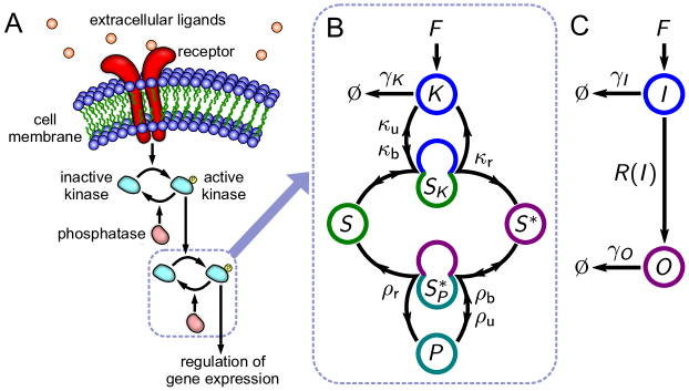
Figure 1: Schematic of a signaling cascade. A: A signaling pathway involving cascades of kinase phosphorylation, activated by a receptor embedded in the cell membrane which responds to extracellular ligands. B: A close-up of one enzymatic push-pull loop within the cascade. Kinase ($K$) phosphorylates the substrate ($S$), converting it to active form ($S^{\ast}$), while phosphatase ($P$) reverts it to the original form through dephosphorylation. $S_{K}$ and $S^{\ast}_{P}$ represent the substrate in complex with the kinase and phosphatase respectively. The rate parameters labeling the reaction arrows are described in the text. The input $I=K+S_{K}$ and output $O=S^{\ast}+S^{\ast}_{P}$. C: A minimal signaling circuit, involving an input species $I$ and output species $O$, related by the production rate function $R(I)$.

Results and Discussion

Theoretical framework for a minimal signaling circuit. To obtain the central results, we start with an example which illustrates the efficacy of the WK theory, and suggests a way to a more detailed, realistic model of the enzymatic push-pull loop. Consider a small portion of a signaling pathway [Fig. 1C], involving two chemical species: one with time-varying population $I(t)$ (the “input”), and another one with population $O(t)$ (the “output”) whose production depends on $I(t)$. These could be, for example, the active, phosphorylated forms of two kinases within a signaling cascade, with $O$ downstream of $I$. The upstream part of the pathway contributes an effective production rate $F$ for species $I$, which in general can be time-dependent, though for now we will make $F$ constant. The output $O$ is produced by a reaction, $I\xrightarrow{R(I)}I+O$, with a rate $R(I(t))$ that depends on the input. The species are deactivated with respective rates $\gamma_{I}$ and $\gamma_{O}$, mimicking the role of the phosphatases. The input $I(t)$ will vary over a characteristic time scale $\gamma_{I}^{-1}$, fluctuating around the mean $\bar{I}=F/\gamma_{I}$. The output deactivation rate sets the response time scale $\gamma_{O}^{-1}$ over which $O(t)$ can react to changes in the input. The dynamical equations, within a continuum, chemical Langevin (CL) description Gillespie (2000), are given by:

$$\frac{dI}{dt}=F-\gamma_{I}I+n_{I},\quad\frac{dO}{dt}=R(I)-\gamma_{O}O+n_{O},$$ (1)

where the additive noise contribution $n_{\alpha}(t)=\sqrt{2\gamma_{\alpha}\bar{\alpha}}\,\eta_{\alpha}(t)$, with $\alpha=I,O$ and $\bar{\alpha}$ denoting the mean of population $\alpha$. The function $\eta_{\alpha}(t)$ is Gaussian white noise with correlation $\langle\eta_{\alpha}(t)\eta_{\alpha^{\prime}}(t^{\prime})\rangle=\delta_{\alpha\alpha^{\prime}}\delta(t-t^{\prime})$. The $\langle\>\rangle$ brackets denote an average over the ensemble of all possible noise realizations.

For small deviations $\delta\alpha(t)=\alpha(t)-\bar{\alpha}$ from the mean populations $\bar{\alpha}$, Eq. (1) can be solved using a linear approximation, where we expand the rate function to first order, $R(I(t))\approx R_{0}\bar{I}+R_{1}\delta I(t)$, with coefficients $R_{0}$, $R_{1}>0$. (We will return later to the issues of nonlinearity and discrete populations.) The result is:

$$\delta I(t) =\int_{-\infty}^{t}dt^{\prime}\,e^{-\gamma_{I}(t-t^{\prime})}n_{I}(t^{\prime}),$$ (2)

$$\delta O(t) =\int_{-\infty}^{t}dt^{\prime}\,\frac{R_{1}}{G}e^{-\gamma_{O}(t-t^{\prime})}\left[G\delta I(t^{\prime})+\frac{G}{R_{1}}n_{O}(t^{\prime})\right],$$

where in the second line we have introduced an arbitrary scaling factor $G>0$ (to be defined below) inside the brackets, and divided through by $G$ outside the brackets. The solution for $\delta O(t)$ has the structure of a linear noise filter equation: $\tilde{s}(t)=\int_{-\infty}^{t}dt^{\prime}H(t-t^{\prime})c(t^{\prime})$, with $c(t)=s(t)+n(t)$. In this analogy, we have a signal $s(t)\equiv G\delta I(t)$ together with a noise term $n(t)\equiv GR^{-1}n_{O}(t)$ forming a corrupted signal $c(t)$. The output $\tilde{s}(t)\equiv\delta O(t)$ is produced by convolving $c(t)$ with a linear filter kernel $H(t)\equiv R_{1}G^{-1}\exp(-\gamma_{O}t)$. As a consequence of causality, the integrals in Eq. (2) run over $t^{\prime}<t$, so the filtered output $\tilde{s}(t)$ at any time $t$ depends only on $c(t^{\prime})$ from the past.

The utility of mapping the push-pull system onto a noise filter comes from the application of WK theory, which is designed to solve a key optimization problem: out of all possible causal, linear filters $H(t)$, what is the optimal function $H_{\text{\tiny WK}}(t)$ that minimizes the differences between the output $\tilde{s}(t)$ and input $s(t)$ time series. In our example, this means having $\delta O(t)$ reproduce as accurately as possible the scaled input signal $G\delta I(t)$. Specifically, we would like to minimize the relative mean-squared error $E=\langle(\tilde{s}-s)^{2}\rangle/\langle s^{2}\rangle$. For a particular $\delta I(t)$ and $\delta O(t)$, the value of $E$ is smallest when $G=\langle(\delta O)^{2}\rangle/\langle\delta O\delta I\rangle$, which we will use to define the gain $G$. In this case $E$ reduces to $E=1-\langle\delta O\delta I\rangle^{2}/(\langle(\delta O)^{2}\rangle\langle(\delta I)^{2}\rangle)$. The great achievement of Wiener Wiener (1949) and Kolmogorov Kolmogorov (1941) was to show that $H_{\text{\tiny WK}}$ satisfies the following Wiener-Hopf equation:

$$C_{cs}(t)=\int_{-\infty}^{t}dt^{\prime}\,H_{\text{\tiny WK}}(t-t^{\prime})C_{cc}(t^{\prime}),\quad t>0$$ (3)

where $C_{xy}(t)\equiv\langle x(t^{\prime})y(t^{\prime}+t)\rangle$ is the correlation between points in time series $x$ and $y$, assumed to depend only on the time difference $t$. Given $C_{cs}$ and $C_{cc}$, which are properties of the signal $s(t)$ and noise $n(t)$, it is possible to solve Eq. (3) for $H_{\text{\tiny WK}}$. The corresponding minimum value of the error $E$ is:

$$E_{\text{\tiny WK}}=1-\frac{1}{C_{ss}(0)}\int_{0}^{\infty}dt\,H_{\text{\tiny WK}}(t)C_{cs}(t).$$ (4)

The solution of the Wiener-Hopf equation requires the following correlation functions, which can be derived from Eq. (2): $C_{ss}(t)=C_{cs}(t)=G^{2}\bar{I}\exp(-\gamma_{I}|t|)$, $C_{nn}(t)=2G^{2}\bar{I}\delta(t)/(\gamma_{I}\Lambda)$, and $C_{cc}(t)=C_{ss}(t)+C_{nn}(t)$, where the parameter $\Lambda\equiv R_{1}^{2}/(R_{0}\gamma_{I})$. Plugging these into Eq. (3), we can solve for the optimal filter function by assuming a generic ansatz $H_{\text{\tiny WK}}(t)=\sum_{i=1}^{N}A_{i}\exp(-\lambda_{i}t)$, finding the unknown coefficients $A_{i}$ and rate constants $\lambda_{i}$ by comparing the left and right sides of the equation. In our case, a single exponential ($N=1$) is sufficient to exactly satisfy Eq. (3) (see details in Appendix A), and we get $H_{\text{\tiny WK}}(t)=\gamma_{I}(\sqrt{1+\Lambda}-1)\exp(-\gamma_{I}\sqrt{1+\Lambda}\,t)$. The conditions for achieving WK optimality, $H(t)=H_{\text{\tiny WK}}(t)$, are then:

$$\gamma_{O}=\gamma_{I}\sqrt{1+\Lambda},\qquad G=\frac{R_{1}}{\gamma_{I}(\sqrt{1+\Lambda}-1)}.$$ (5)

From Eq. (4) the minimum relative error is:

$$E_{\text{\tiny WK}}=\frac{2}{1+\sqrt{1+\Lambda}}.$$ (6)

The fidelity between output and input is described through a single dimensionless optimality control parameter, $\Lambda$. It can be broken up into two multiplicative factors, reflecting two physical contributions: $\Lambda=(R_{0}/\gamma_{I})(R_{1}/R_{0})^{2}$. The first term, $R_{0}/\gamma_{I}$, is a burst factor, measuring the mean number of output molecules produced per input molecule during the active lifetime of the input molecule. The second term, $(R_{1}/R_{0})^{2}$, is a sensitivity factor, reflecting the local response of the production function $R(I)$ near $\bar{I}$ (controlled by the slope $R_{1}=R^{\prime}(\bar{I})$) relative to the production rate per input molecule $R_{0}=R(\bar{I})/\bar{I}$. Note that $(R_{1}/R_{0})^{2}>1$ only if $R(I)$ is globally nonlinear, since physical production functions satisfy $R(I)\geq 0$ for all $I\geq 0$. If $R(I)$ is perfectly linear, $R(I)=R_{0}I$, then $R_{1}=R_{0}$, and $(R_{1}/R_{0})^{2}=1$. Thus the limit of efficient noise suppression, $\Lambda\gg 1$, where $E_{\text{\tiny WK}}$ becomes small, can be achieved by making the burst factor $R_{0}/\gamma_{I}\gg 1$ and/or enhancing the sensitivity $(R_{1}/R_{0})^{2}\gg 1$, at the cost of introducing nonlinear effects (discussed in detail below). For optimality to be realized, we additionally need an appropriate separation of scales [Eq. (5)] between the characteristic time of variations in the input signal, $\gamma_{I}^{-1}$, and the response time of the output, $\gamma_{O}^{-1}$. The latter should be faster by a factor of $\sqrt{1+\Lambda}$. The scaling $E_{\text{\tiny WK}}\sim\Lambda^{-1/2}$ for large $\Lambda$ is the same as the burst factor scaling of the target population variance in biochemical negative feedback networks intended to maintain homeostasis and suppress fluctuations Lestas et al. (2010). The slow $\Lambda^{-1/2}$ decay in both cases, compared to the more typical scaling of variance with $\Lambda^{-1}$ (inversely proportional to the number of signaling molecules produced) reflects the same underlying physical challenge: the difficulty of suppressing or filtering noise in stochastic reaction networks.

The error $E$ defined above is based on the instantaneous difference between the input $s(t)$ and output $\tilde{s}(t)$ time series. One of the powerful features of the WK formalism is that it naturally extends error minimization to cases where the goal is extrapolating the future signal, where we seek to minimize the difference between $\tilde{s}(t)$ and $s(t+\alpha)$ for some $\alpha>0$ Bode and Shannon (1950). Given the time delays inherent in many biological responses, particularly where feedback is involved, such predictive noise filtering has significant applications Bialek et al. (2001), which we will explore in subsequent work. For now, we confine ourselves to the instantaneous error, which is sufficient to treat the kinase-phosphatase push-pull loop.

We also note that there is no unique measure of signal fidelity. Besides $E$, one can optimize the mutual information between the output and input species in the cascade Levine et al. (2007). For example, in the two-component cascade with nonlinear regulation, considered below, a spectral expansion of the master equation allows for efficient numerical optimization of the system parameters for particular forms of the rate function, maximizing the mutual information Mugler et al. (2009); Walczak et al. (2009).

Effects of nonlinearity and discrete populations. For the subclass of Gaussian-distributed signal $s(t)$ and noise $n(t)$ time series (as is the case within the CL picture), the WK filter derived above, based on the linearization of the CL, is optimal among all possible linear or nonlinear filters Bode and Shannon (1950). If the system fluctuates around a single stable state, and the copy numbers of the species are large enough that their Poisson distributions converge to Gaussians (mean populations $\gtrsim 10$), the signal and noise are usually approximately Gaussian. However, the rate function $R(I)$ will never be perfectly linear in practice, and thus one needs to consider how nonlinearities in $R(I)$ will affect the minimal $E$. In addition, the discrete nature of population changes, which becomes important at lower copy numbers, has to be explicitly taken into consideration. Surprisingly, the WK result of Eq. (6) can be generalized even to cases where the linear, continuum assumptions underlying WK theory no longer hold.

Starting from the exact master equation, valid for discrete populations and arbitrary $R(I)$, we have rigorously solved the general optimization problem for the error $E$ between output and input using the principles of umbral calculus Roman (2005). The detailed proof is in Appendix B, but the main results are as follows. Any function $R(I)$ can be expanded in terms of a set of polynomials $v_{n}(I)$ as $R(I)=\sum_{n=0}^{\infty}\sigma_{n}v_{n}(I)$. The $v_{n}(I)$ are polynomials of degree $n$, given by

$$v_{n}(I)=\sum_{m=0}^{n}(n-m)!\left(-\bar{I}\right)^{m}\binom{n}{m}\binom{I}{n-m},$$ (7)

and the coefficients $\sigma_{n}$ are related to moments of $R(I)$, $\sigma_{n}=\langle v_{n}(I)R(I)\rangle/(\bar{I}^{n}n!)$. The average is taken with respect to the Poisson distribution ${\cal P}(I)=\bar{I}^{I}\exp(-\bar{I})/I!$. The first two polynomials are $v_{0}=1$ and $v_{1}=I-\bar{I}$, giving $\sigma_{0}=\langle R(I)\rangle$ and $\sigma_{1}=\langle(I-\bar{I})R(I)\rangle/\bar{I}$. Remarkably, the relative error $E$ has an exact analytical form in terms of the $\sigma_{n}$,

$$E=1-\frac{\bar{I}\gamma_{O}^{2}\sigma_{1}^{2}}{(\gamma_{I}+\gamma_{O})^{2}}\left[\gamma_{O}\sigma_{0}+\sum_{n=1}^{\infty}\sigma_{n}^{2}\frac{\gamma_{O}n!\bar{I}^{n}}{\gamma_{O}+n\gamma_{I}}\right]^{-1}.$$ (8)

This expression is bounded from below by

$$E\geq E_{\text{opt}}\equiv\frac{2}{1+\sqrt{1+\tilde{\Lambda}}},$$ (9)

where $\tilde{\Lambda}=\bar{I}\sigma_{1}^{2}/(\sigma_{0}\gamma_{I})$. The equality is only reached when $\gamma_{O}=\gamma_{I}\sqrt{1+\tilde{\Lambda}}$ and $R(I)$ has an optimal linear form, $R_{\text{opt}}(I)=\sigma_{0}+\sigma_{1}(I-\bar{I})$, with all $\sigma_{n}=0$ for $n\geq 2$. In this optimal case, $\sigma_{0}=R_{0}\bar{I}$ and $\sigma_{1}=R_{1}$, and hence $\tilde{\Lambda}=\Lambda$, $E=E_{\text{opt}}=E_{\text{\tiny WK}}$ from Eq. (6).

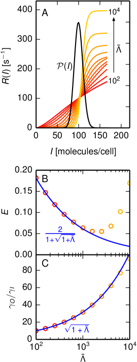
Figure 2: Optimal noise reduction in the minimal signaling circuit (Fig. 1C). A: Numerical optimization results for the Hill production function $R(I)$ that minimizes relative error $E$ between input and output, with each color corresponding to different values of the parameter $\tilde{\Lambda}=10^{2}-10^{4}$ (see text for other parameters). The input probability distribution ${\cal P}(I)$ is superimposed in black (the height scale is arbitrary). B: For each value of $\tilde{\Lambda}$ from panel A, circles show the minimal $E$. The lower bound $E_{\text{opt}}$ [Eq. (9)] is drawn as a blue curve. C: Analogous to panel B, but showing the ratio $\gamma_{O}/\gamma_{I}$ at which the minimum $E$ is achieved. The blue curve shows the WK prediction for this ratio, $\gamma_{O}/\gamma_{I}=\sqrt{1+\tilde{\Lambda}}$.

Making $\tilde{\Lambda}$ large, for example by increasing $\sigma_{1}$, is desirable for better signal transduction, but with a caveat. We can keep $E$ near $E_{\text{opt}}$ even for a globally nonlinear $R(I)$ so long as $R(I)$ remains approximately linear in the vicinity of the mean $\bar{I}$, and the nonlinear corrections $\sigma_{n}$ for $n\geq 2$ are negligible. Large $\sigma_{1}$ can be achieved through a highly sigmoidal input-output response, known as ultrasensitivity, which is biologically realizable in certain regimes of signaling cascades Goldbeter and Koshland (1981). However, our theory predicts that as $R(I)$ goes to the extreme limit of a step-like profile around $\bar{I}$, $E$ should become significantly higher than $E_{\text{opt}}$, and the benefits of ultrasensitivity vanish. The reason for this is that letting $\sigma_{1}$ become arbitrarily large (making the step sharper) necessarily implies that $R(I)$ eventually deviates substantially from $R_{\text{opt}}(I)$. We know that any physically sensible $R(I)$ satisfies the constraint $R(I)\geq 0$ for $I\geq 0$. If $\sigma_{1}\gg\sigma_{0}/\bar{I}$ and $\sigma_{n}\approx 0$ for $n\geq 2$, the function $R(I)$ would be negative for $I\lesssim\bar{I}-\sigma_{0}/\sigma_{1}$, violating the physical constraint. Hence the coefficients $\sigma_{n}$ for $n\geq 2$ must be non-negligible when $\sigma_{1}$ is sufficiently large, leading to $E>E_{\text{opt}}$.

We can illustrate this result numerically for $R(I)$ that have the form of a Hill function, $R(I)=R_{\text{s}}(I/I_{0})^{n_{\text{H}}}/(1+(I/I_{0})^{n_{\text{H}}})$, defined by the three parameters $R_{\text{s}}$, $I_{0}$, and ${n_{\text{H}}}$. This represents a typical sigmoidal behavior in biochemical systems, with a small production rate for $I\ll I_{0}$ switching over to a saturation level $R_{\text{s}}$ for $I\gg I_{0}$. We performed a numerical minimization of $E$ (evaluated using Eq. (8)) over the parameter space, at fixed $F$, $\gamma_{I}$, $\sigma_{0}$, and $\tilde{\Lambda}$. Using Eq. (8) is numerically extremely efficient, since the coefficients $\sigma_{n}$ typically decay quite rapidly, allowing the infinite sum to converge after a small ($<10$) number of terms. Fixing $\sigma_{0}$ and $\tilde{\Lambda}$ is equivalent to specifying the first two moments of $R(I)$, which in turn defines a curve in the three-dimensional parameter space of $R_{\text{s}}$, $I_{0}$, and ${n_{\text{H}}}$. After numerically solving for this curve, the minimization procedure consists of searching along the curve (and varying the free system parameter $\gamma_{O}$) to find the parameter set that yields the smallest $E$. Fig. 2A shows optimization results for $F=1$ s^-1, $\gamma_{I}=0.01$ s^-1, $\sigma_{0}=100$ s^-1, and varying $\tilde{\Lambda}$, with the optimal Hill function $R(I)$ (the one with smallest $E$) at each $\tilde{\Lambda}$ drawn in a different color. The corresponding minimal values of $E$ are shown in Fig. 2B as circles in the same colors, with $E_{\text{opt}}$ using Eq. (9) drawn as a blue curve for comparison. Larger values of $\tilde{\Lambda}$ have optimal $R(I)$ profiles that are increasingly step-like, with steeper slopes near $\bar{I}$. For the range $\tilde{\Lambda}=10^{2}-10^{3}$ the maximum slope ($\approx\sigma_{1}$) is still small enough that $R(I)$ remains approximately linear across the entire $I$ range where ${\cal P}(I)$ is non-negligible (the distribution is superimposed in Fig. 2A). Hence minimal $E$ values are very close to $E_{\text{opt}}$, decreasing with $\tilde{\Lambda}$. The ratios $\gamma_{O}/\gamma_{I}$ at which these minimal $E$ values occur, shown in Fig. 2C, are nearly equal to the predicted value $\sqrt{1+\tilde{\Lambda}}$ (blue curve). We can estimate that this near-optimality will persist up to $\sigma_{1}\approx\sigma_{0}/(3\sqrt{\bar{I}})$, since that is roughly the slope of an $R(I)$ that rises from zero near the left edge of ${\cal P}(I)$ (at $I\approx\bar{I}-3\sqrt{\bar{I}}$) to a value of $\sigma_{0}$ at $I=\bar{I}$. For $\sigma_{1}\gtrsim\sigma_{0}/(3\sqrt{\bar{I}})$, or equivalently $\tilde{\Lambda}\gtrsim\sigma_{0}/(9\gamma_{I})=1.1\times 10^{3}$, the nonlinearity of $R(I)$ becomes appreciable around $\bar{I}$, distorting the output signal and leading to minimal $E$ noticeably larger than $E_{\text{opt}}$, and actually increasing with $\tilde{\Lambda}$. Thus moving towards the ultrasensitive limit $\tilde{\Lambda}\to\infty$ is initially beneficial for noise filtering, but only up to a point: $R(I)$ does not have to be globally linear, but local linearity of $R(I)$ near $\bar{I}$, which can be satisfied readily, is best for accurate signal transduction.

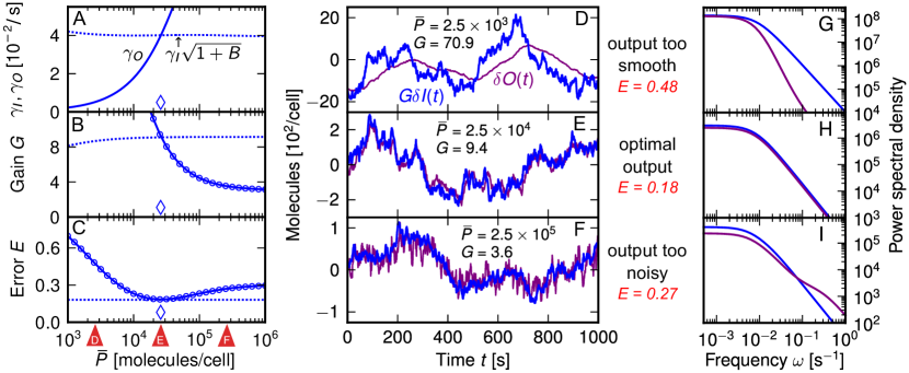
Figure 3: A: $\gamma_{O}$ (solid curve) and $\gamma_{I}\sqrt{1+\Lambda}$ (dashed curves), based on the mapping in Eq. (11), for $\Lambda=100$. The $\bar{P}$ value at the intersection of the solid and dashed curves, where the WK optimality conditions are fulfilled, is indicated by a diamond. B: Gain $G$ (solid line: CL theory; circles: KMC simulations) for the same $\Lambda$ value as in panel A, versus the WK optimal value for $G$ (dashed line) given by Eq. (5). C: Same as panel B, but showing error $E$ versus the WK optimal prediction $E_{\text{\tiny WK}}$ (dashed line) from Eq. (6). D-F: Sample trajectories for the scaled input $G\delta I(t)$ (blue) and the output $\delta O(t)$ (purple) from KMC simulations of the push-pull loop, for $\Lambda=100$ ($\bar{S}=8\times 10^{4}$) and three different values of $\bar{P}$. These $\bar{P}$ values are marked by red triangles under panel C, and correspond to cases where, relative to the input, the output is too smooth (D), optimal (E), and too noisy (F). G-I: Power spectral densities of the scaled input $G\delta I(t)$ (blue) and the output $\delta O(t)$ (purple) for the three cases shown in panels D-F.

Enzymatic push-pull loop can act as an optimal WK filter. The system considered so far is the simplest realization of a signaling circuit, in the sense that it involves only two species, related through a single phenomenological production function, $R(I)$. In reality, an enzymatic push-pull loop involves intermediates—complexes of the substrate with the kinase or phosphatase—whose binding, unbinding, and catalytic reactions all contribute to the stochastic nature of signal transmission. Can the WK theoretical framework be used to describe optimality in this complicated context? Let us consider a more microscopic model of the loop reaction network [Fig. 1B]. The active kinase is either free ($K$) or bound to substrate ($S_{K}$). The input $I$ is defined as the total active kinase population $I=K+S_{K}$. Upstream modules control kinase activation and deactivation, described by rates $F$ and $\gamma_{K}$ respectively. The kinase can phosphorylate the substrate, converting it from inactive ($S$) to active ($S^{\ast}$) form. Analogously, in the reverse direction, free phosphatases ($P$) form complexes with the active substrate ($S^{\ast}_{P}$), which lead to dephosphorylation, returning the substrate to inactive form. The output $O$ is the total active substrate population $O=S^{\ast}+S^{\ast}_{P}$. The reactions for substrate modification, with corresponding rate constants, are:

$$\begin{split}K+S&\xrightleftharpoons[\kappa_{\text{u}}]{\kappa_{\text{b}}}S_{K}\xrightarrow{\kappa_{\text{r}}}K+S^{\ast}\\ P+S^{\ast}&\xrightleftharpoons[\rho_{\text{u}}]{\rho_{\text{b}}}S^{\ast}_{P}\xrightarrow{\rho_{\text{r}}}P+S.\end{split}$$ (10)

We chose representative rate values based on a model of the MAP kinase cascade Schoeberl et al. (2002) (all units are in s^-1): $\kappa_{\text{b}}=\rho_{\text{b}}=10^{-5}$, $\kappa_{\text{u}}=0.02$, $\rho_{\text{u}}=0.5$, $\kappa_{\text{r}}=3$, $\rho_{\text{r}}=0.3$, $F=1$. The rate $\gamma_{K}$ in the model controls the characteristic time scale over which the input signal varies. We let $\gamma_{K}=0.01$ s^-1, which sets this scale to minutes. Mean free substrate and phosphatase populations (which together with the rates determine all equilibrium population values) are in the ranges: $\bar{S}\sim 10^{4}-10^{5}$, $\bar{P}\sim 10^{3}-10^{6}$ molecules/cell.

We simulated the dynamics of this system numerically using kinetic Monte Carlo (KMC) Gillespie (1977), with sample input and output trajectories shown in Fig. 3D-F for $\bar{S}=8\times 10^{4}$ and three values of $\bar{P}$. As the free phosphatase population is varied, we see different degrees of signal fidelity, with the closest match between $\delta O(t)$ and $G\delta I(t)$ for the intermediate case in Fig. 3E. Are we seeing behavior similar to an optimal WK filter? As detailed in Appendix C, we can approximately map the phosphorylation cycle to a noise filter using the same method as in our first example: starting from the full dynamical equations in the linear CL approximation, we derive the correlation functions required to solve the Wiener-Hopf relation, Eq. (3). The effective parameters resulting from the mapping are:

$$\gamma_{O} =\frac{\rho_{\text{r}}\rho_{+}}{\sqrt{\rho^{2}-2\rho_{\text{r}}\rho_{+}}},\>R_{1}=\frac{\kappa_{\text{r}}\kappa_{+}\rho}{\kappa\sqrt{\rho^{2}-2\rho_{\text{r}}\rho_{+}}},\>\gamma_{I}=\frac{\kappa_{-}\gamma_{K}}{\kappa},$$

$$\Lambda =\frac{\kappa_{\text{r}}\kappa_{+}\kappa^{2}\rho^{2}}{\gamma_{K}\kappa_{-}(\rho^{2}(\kappa^{2}-\kappa_{\text{r}}\kappa_{+})-\rho_{\text{r}}\rho_{+}\kappa^{2})},$$ (11)

where $\kappa_{+}=\kappa_{\text{b}}\bar{S}$, $\kappa_{-}=\kappa_{\text{u}}+\kappa_{\text{r}}$, $\kappa=\kappa_{+}+\kappa_{-}$, $\rho_{+}=\rho_{\text{b}}\bar{P}$, $\rho_{-}=\rho_{\text{u}}+\rho_{\text{r}}$, and $\rho=\rho_{+}+\rho_{-}$. Eq. (11) is valid in the regime $\bar{K}=F/\gamma_{K}\ll\bar{S},\bar{P}$, with corrections of order $\bar{K}/\bar{S}$ and $\bar{K}/\bar{P}$ shown in Appendix C. Such a mapping allows us to use WK results in Eqs. (5) and (6) to predict the conditions for optimality and the minimal possible $E$. Figs. 3A-B show the left (solid lines) and right-hand (dashed lines) sides of both conditions in Eq. (5) as a function of $\bar{P}$ for $\Lambda=100$ ($\bar{S}=8\times 10^{4}$). The $\bar{P}$ value at the intersections, where the conditions are fulfilled, is marked by a diamond. Fig. 3C shows that exactly at this value $E$ achieves a minimum, given by $E_{\text{\tiny WK}}$ from Eq. (6) (dashed line). The CL approximation (solid curves) and KMC simulations (circles) are in excellent agreement. Thus, the phosphorylation cycle can indeed be tuned to behave like an optimal WK noise filter, even for a realistic signaling model. In light of the mapping in Eq. (11), we can now understand the behavior of the trajectories in Fig. 3D-F, which correspond to $\Lambda=100$. In panel D, where $\bar{P}=2.5\times 10^{3}$, we have $\gamma_{O}\ll\gamma_{I}\sqrt{1+\Lambda}$ [Fig. 3A], and the output $\delta O(t)$ becomes excessively smooth, since it cannot respond quickly enough to changes in the input signal $G\delta I(t)$. The corresponding power spectral density (PSD) of the output, shown in panel G, is smaller at high frequencies compared to the PSD of the input. In panel F, we have the opposite situation of $\gamma_{O}\gg\gamma_{I}\sqrt{1+\Lambda}$ at $\bar{P}=2.5\times 10^{5}$. The output response is too rapid, generating additional noise that obscures the signal. In this case the output PSD (panel I) has an extra high frequency contribution relative to the input PSD. Panel E represents the optimal intermediate $\bar{P}=2.5\times 10^{4}$, where $\gamma_{O}=\gamma_{I}\sqrt{1+\Lambda}$ and the WK conditions are fulfilled. The input and output PSDs (panel H) are similar at all frequencies.

The minimum of $E$ in Fig. 3C is shallow, meaning that near-optimal filtering persists even when the phosphatase population is not precisely tuned to the WK condition. For $\bar{P}$ values that vary nearly five-fold between $\bar{P}=1.3-6.3\times 10^{4}$, the error $E$ remains within 5% of the minimum value $E_{\text{\tiny WK}}$. Another aspect of the filter’s robustness can be highlighted by perturbing the enzymatic parameters $\kappa_{\text{b}}$, $\rho_{\text{b}}$, $\kappa_{\text{u}}$, $\rho_{\text{u}}$, $\kappa_{\text{r}}$, and $\rho_{\text{r}}$. If we randomly vary all these parameters within a range between 0.1 and 10 times the values listed above after Eq. (10), and calculate the resulting conditions for WK optimality [Eq. (5)] for each new parameter set, we obtain the results in Fig. 4. For a given $\bar{P}$, the shaded intervals in the figure correspond to the 68% confidence intervals on the input kinase frequency scale $\gamma_{K}$ and the mean substrate population $\bar{S}$ at optimality. Thus, for a broad range of biologically relevant enzymatic parameters, we get a sense of how the populations of $\bar{P}$ and $\bar{S}$ must complement each other, and an associated time scale $\gamma_{K}^{-1}$ reflecting how quickly the input signal can vary and still be accurately transduced. From the trends in Fig. 4, we see that to get the system to respond to more rapidly varying signals, we need larger populations of $\bar{P}$ and $\bar{S}$. As a concrete example, for the hyperosmolar glycerol (HOG) signaling pathway in yeast, discussed further in the next section, kinase substrates have cell copy numbers of between $6\times 10^{1}$ and $7\times 10^{3}$, while the PTP and PTC phosphatases that have been identified as targeting the pathway are present in cell copy numbers between $1.5\times 10^{2}$ and $2\times 10^{4}$ Ghaemmaghami et al. (2003). Using these population scales as a rough guide for $\bar{S}$ and $\bar{P}$ (ignoring complications like multiple phosphorylation steps and sharing of phosphatases between different pathways) we see from Fig. 4 that the corresponding $\gamma_{K}\sim 10^{-4}-10^{-2}$ s^-1. This range of optimal time scales is consistent with the experimental observation that the HOG pathway can faithfully transduce osmolyte signals at frequencies $\lesssim 5\times 10^{-3}$ s^-1 Mettetal et al. (2008).

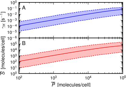
Figure 4: Conditions for WK optimality as the enzymatic push-pull loop parameters are varied. A: The solid blue curve shows the relation between mean phosphatase population $\bar{P}$ and the characteristic frequency scale $\gamma_{K}$ over which the active kinase input signal varies. This is at WK optimality [Eq. (5)], using the mapping of Eq. (11) and the parameter values $\kappa_{\text{b}}$, $\rho_{\text{b}}$, $\kappa_{\text{u}}$, $\rho_{\text{u}}$, $\kappa_{\text{r}}$, $\rho_{\text{r}}$ listed in the text after Eq. (10). The shaded region between the dashed curves shows the 68% confidence interval for achieving WK optimality, resulting from randomly perturbing all the parameter values so that they can be up to ten-fold smaller or larger. B: Analogous to panel A, but showing the relation between $\bar{P}$ and substrate population $\bar{S}$ at WK optimality.

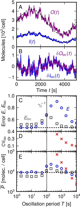
Figure 5: A: sample KMC simulation trajectories for $I(t)$ (solid blue) and $O(t)$ (solid purple) in a $\Lambda=10$ system driven by an oscillatory upstream flux $F(t)$ (see text for parameters). Dashed lines are local means $I_{\text{loc}}(t)$ and $O_{\text{loc}}(t)$. B: for trajectories in A, the deviations from local means, $\delta I_{\text{loc}}(t)$ (blue) and $\delta O_{\text{loc}}(t)$ (purple). C-E: Results calculated from KMC for a system with $\Lambda=10$ and oscillatory $F(t)$ at varying driving periods $T$. $\gamma_{I}^{-1}$ is marked by a vertical dashed line. C: The minimum errors $E$ (circles) and $E_{\text{loc}}$ (squares). $E_{\text{\tiny WK}}$ is marked by a horizontal dashed line. D: The minimum local coefficient of variation $\text{CV}_{\text{loc}}=\sqrt{\langle(\delta O_{\text{loc}}/\bar{O}_{\text{loc}})^{2}\rangle}$. E: The mean phosphatase population values $\bar{P}$ at which the minima shown in panels C and D are achieved ($E$: circles, $E_{\text{loc}}$: squares, $\text{CV}_{\text{loc}}$: crosses). The $\bar{P}$ value for WK optimality is marked by a horizontal dashed line.

Noise filtration in a push-pull loop driven by oscillatory input. Remarkably, since Eq. (11) is independent of $F$, the system can serve as an optimal filter for a range of $F$ values, so long as the condition $F/\gamma_{K}\ll\bar{S},\bar{P}$ is satisfied. This regime, involving saturated kinases and unsaturated phosphatases, has been previously identified as a candidate for efficient signal transmission by Gomez-Uribe et al. Gomez-Uribe et al. (2007). To check the filter operation with varying upstream flux, we used a time-dependent $F(t)$, driving the system with oscillatory input. This is motivated by microfluidic experimental setups Mettetal et al. (2008); Hersen et al. (2008), where the HOG pathway of yeast was probed by exposing the cells to periodic osmolyte pulses. In the experiments, the input signal is the extracellular osmolyte concentration, and the output is the degree to which the activated kinase Hog1 localizes in the nucleus, where it initiates a transcriptional response to the osmolar shock. Though the biochemical network relating the output to input consists of a complex series of enzymatic push-pull loops, the overall behavior was quantified through response functions in terms of input signal frequency Mettetal et al. (2008), related to the Fourier transforms of the input-output correlation functions. Such correlation functions are the basic ingredients in assessing filter optimality in the WK theory. Here, we will focus only on a single push-pull loop, and use input at varying frequencies to determine whether $E_{\text{\tiny WK}}$ remains a meaningful constraint on filter performance even for non-stationary signals. In Fig. 5A we show a sample $I(t)$ and $O(t)$ KMC trajectory at optimality for $F(t)=\bar{F}(1+A\sin(2\pi t/T))$, with $\bar{F}=1$ s^-1, $A=0.5$, and $T=5000$ s. The input has two characteristic time scales, $T$ and $\gamma_{I}^{-1}=10^{2}$ s. For $T\gg\gamma_{I}^{-1}$, we define relative error in terms of deviations from local, time-dependent means: $E_{\text{loc}}$ defined using $\delta I_{\text{loc}}=I(t)-\bar{I}_{\text{loc}}(t)$ and $\delta O_{\text{loc}}=O(t)-\bar{O}_{\text{loc}}(t)$ [Fig. 5B], where $\bar{I}_{\text{loc}}(t)=\bar{I}F(t)/\bar{F}$, $\bar{O}_{\text{loc}}(t)=\bar{O}F(t)/\bar{F}$ are shown as dashed curves in Fig. 5A. Fig. 5C shows KMC results for minimum $E$ and minimum $E_{\text{loc}}$ as a function of $T$ for a system tuned to optimality with $\Lambda=10$. The values of $\bar{P}$ at which these minima are achieved are shown in Fig. 5E. At $T>\gamma_{I}^{-1}$ we find $E_{\text{loc}}<E$, since both the input and output have time to adjust to the slowly varying local means. In fact, the minimum $E_{\text{loc}}$ approaches $E_{\text{\tiny WK}}$ for $T\gg\gamma_{I}^{-1}$, as optimality is unaffected by the slow oscillation in $F(t)$. The $\bar{P}$ where the minimum $E_{\text{loc}}$ occurs also approaches the value predicted by WK theory (Fig. 5E). The filter transduces the signal with high fidelity. In the opposite limit of small $T<\gamma_{I}^{-1}$, the rapidly varying $F(t)$ essentially averages out, since neither the input nor the output have time to respond to the sharp changes in $F(t)$. Thus the system sees an effective constant flux $\bar{F}$. Here $E$, the error estimate with respect to the global mean, is more relevant than $E_{\text{loc}}$. In this regime the minimum $E<E_{\text{loc}}$, $E$ approaches $E_{\text{\tiny WK}}$ for $T\ll\gamma_{I}^{-1}$, and the $\bar{P}$ value where $E$ is minimized agrees with the WK prediction.

The two regimes in system behavior, with a changeover at the time scale $\gamma_{I}^{-1}$, reflect the fact that the enzymatic loop acts an effective low-pass filter Detwiler et al. (2000); Hersen et al. (2008): it can accurately transmit the low frequency component of $F(t)$, but integrates over the high-frequency portion above a certain bandwidth. The overall bandwidth of a cascade of push-pull loops has been experimentally characterized for the yeast HOG pathway, yielding a value of $\omega_{b}\approx 5\times 10^{-3}$ s^-1 Hersen et al. (2008). Using this as a rough estimate of the bandwidth scale $\gamma_{I}$ in individual loops, we could expect to see a changeover between the two regimes depending on whether the driving frequency is much slower or faster than $\omega_{b}$. Regardless of the magnitude of the driving frequency, both $E$ and $E_{\text{loc}}$ always remain greater than $E_{\text{\tiny WK}}$, so the latter remains a bound on noise filter efficiency even for dynamic input.

More generally, the low-pass filtering property of the enzymatic loop can be fine-tuned to optimize other signal transmission characteristics besides $E$ and $E_{\text{loc}}$. These two errors are minimized when the output fluctuations ($\delta O$ or $\delta O_{\text{loc}}$) closely follow the scaled input fluctuations ($G\delta I$ or $G\delta I_{\text{loc}}$). However one could imagine biological scenarios where the desired outcome was a smoothed output that mirrored the oscillatory driving signal. In other words we could demand that $O(t)$, as shown for example in Fig. 5A (purple trajectory), deviates minimally from the oscillatory local mean $\bar{O}_{\text{loc}}(t)$ (superimposed dashed line). In this case, the natural quantity to minimize would be a local coefficient of variation, $\text{CV}_{\text{loc}}=\sqrt{\langle(\delta O_{\text{loc}}/\bar{O}_{\text{loc}})^{2}\rangle}$. From the oscillatory KMC simulations described above, we calculate $\text{CV}_{\text{loc}}$, and find that it can be made small in the slow oscillation regime $T\gg\gamma_{I}^{-1}$, as shown in Fig. 5D, which plots the minimum $\text{CV}_{\text{loc}}$ as a function of $T$ for $T\geq 500$ s. From Fig. 5E, which shows the $\bar{P}$ values at which the minimum $\text{CV}_{\text{loc}}$ occurs (crosses), we see that in the large $T$ limit this $\bar{P}$ value is smaller than the WK prediction. This makes sense, since as we know from the case of a constant driving function ($T\to\infty$), illustrated in Fig. 3D, keeping $\bar{P}$ below the WK optimum smooths the output. For systems more complex than the enzymatic loop, smoothed output (homeostasis around a constant mean, or tracking of a driven, time-varying local mean) can be enhanced by introducing some negative feedback mechanism from the output back to the input Lestas et al. (2010). For such negative feedback systems it turns out there exists a mapping onto a different WK filter Hinczewski and Thirumalai (2014).

Conclusions

We have demonstrated the usefulness of a generalized WK filter theory as a way of characterizing signal fidelity in an enzymatic push-pull loop. This basic motif of biological signal transduction can effectively realize an optimal WK noise filter. Through a novel analytical approach, we have generalized WK ideas beyond their original linear context, thus providing fidelity bounds in strongly nonlinear cases, including ultrasensitive production and oscillatory input driving. Even for a complex kinase-phosphatase reaction network with multiple intermediates, the theory predicts the conditions for accurate signal transduction, yielding a bound on the error in terms of a single dimensionless optimality control parameter $\Lambda$. The results highlight how physics and engineering concepts can be use to understand how biology robustly tunes push-pull loops to optimality by setting the copy numbers of phosphatase and substrate molecules. We can relate the wide range of cellular signaling protein copy numbers observed experimentally to optimal time scales on which the cell can accurately transduce the signal, and thus yield an effective physiological response. Since our approach is formulated in terms of correlation functions of signal and noise, quantities readily accessible from both theory and simulation, the current work can be generalized to other complex signaling networks. The ultimate goal is to give insights into the design principles underlying the large, intertwined biochemical pathways that determine how the cell can process and respond to diverse sources of external stimuli.

Appendix A Solving the Wiener-Hopf equation for the optimal filter

Given the correlation functions,

$$\begin{split}C_{ss}(t)&=C_{cs}(t)=G^{2}\bar{I}e^{-\gamma_{I}|t|},\quad C_{nn}(t)=\frac{2G^{2}\bar{I}}{\gamma_{I}\Lambda}\delta(t),\\ C_{cc}(t)&=C_{ss}(t)+C_{nn}(t),\end{split}$$ (12)

we would like to find the optimal filter function $H_{\text{\tiny WK}}(t)$ that satisfies the Wiener-Hopf equation,

$$C_{cs}(t)=\int_{-\infty}^{t}dt^{\prime}\,H_{\text{\tiny WK}}(t-t^{\prime})C_{cc}(t^{\prime}),\quad t>0.$$ (13)

Since $C_{cs}(t)$ and $C_{cc}(t)$ consist of exponential terms and Dirac delta functions, a reasonable ansatz for $H_{\text{\tiny WK}}(t)$ is a sum of $N$ exponentials, $H_{\text{\tiny WK}}(t)=\sum_{i=1}^{N}A_{i}\exp(-\lambda_{i}t)$, with parameters $A_{i}$, $\lambda_{i}$, $i=1,\ldots,N$. Plugging this into Eq. (13), along with the correlation functions from Eq. (12), and carrying out the integral, we find

$$\begin{split}G^{2}\bar{I}e^{-\gamma_{I}t}&=\sum_{i=1}^{N}A_{i}\left[\left(\frac{2G^{2}\bar{I}\gamma_{I}}{\gamma_{I}^{2}-\lambda_{i}^{2}}+\frac{2G^{2}\bar{I}}{\gamma_{I}\Lambda}\right)e^{-\lambda_{i}t}\right.\\ &\qquad\left.+\frac{G^{2}\bar{I}}{\lambda_{i}-\gamma_{I}}e^{-\gamma_{I}t}\right],\quad t>0.\end{split}$$ (14)

Comparing the left-hand and right-hand sides of Eq. (14), we see that the coefficients of the linearly independent exponential terms on both sides must match, giving $N+1$ equations: $N$ coefficients of $\exp(-\lambda_{i}t)$, plus one for $\exp(-\gamma_{I}t)$. Since there are $2N$ unknown parameters in the ansatz, the only value of $N$ that gives a closed set of equations is $N=1$. With this choice of $N$, the resulting two equations are

$$0=A_{1}\left(\frac{2G^{2}\bar{I}\gamma_{I}}{\gamma_{I}^{2}-\lambda_{1}^{2}}+\frac{2G^{2}\bar{I}}{\gamma_{I}\Lambda}\right),\qquad G^{2}\bar{I}=\frac{A_{1}G^{2}\bar{I}}{\lambda_{1}-\gamma_{I}}.$$ (15)

The only physically sensible solution of Eq. (15) for $A_{1}$ and $\lambda_{1}$ (where $|H_{\text{\tiny WK}}(t)|\neq\infty$ as $t\to\infty$) is

$$A_{1}=\gamma_{I}(\sqrt{1+\Lambda}-1),\quad\lambda_{1}=\gamma_{I}\sqrt{1+\Lambda}.$$ (16)

Thus the optimal filter is

$$H_{\text{\tiny WK}}(t)=\gamma_{I}(\sqrt{1+\Lambda}-1)e^{-\gamma_{I}\sqrt{1+\Lambda}\,t}.$$ (17)

Appendix B Optimal signal transduction for the nonlinear, discrete case

To obtain results for the general signal pathway model, where we assume neither linearity of the production function $R(I)$ or a continuum description, we start with an exact equation for the stationary joint distribution ${\cal P}(I,O)$ of the input and output. Using this, we will derive expressions for various moments of the distribution which enter into the relative mean-squared error

$$E=1-\frac{\langle\delta O\delta I\rangle^{2}}{\langle(\delta O)^{2}\rangle\langle(\delta I)^{2}\rangle}=1-\frac{(\langle OI\rangle-\langle O\rangle\langle I\rangle)^{2}}{(\langle O^{2}\rangle-\langle O\rangle^{2})(\langle I^{2}\rangle-\langle I\rangle^{2})}.$$ (18)

From the master equation, ${\cal P}(I,O)$ satisfies

$$\begin{split}&\gamma_{I}\left[(I+1){\cal P}(I+1,O)-I{\cal P}(I,O)\right]\\ &\qquad+F\left[{\cal P}(I-1,O)-{\cal P}(I,O)\right]\\ &\qquad+\gamma_{O}\left[(O+1){\cal P}(I,O+1)-O{\cal P}(I,O)\right]\\ &\qquad+R(I)\left[{\cal P}(I,O-1)-{\cal P}(I,O)\right]=0.\end{split}$$ (19)

Let us define a generating function $H_{I}(z)=\sum_{O=0}^{\infty}z^{O}{\cal P}(I,O)$. By multiplying Eq. (19) by $z^{O}$ and then summing over $O$, we can derive the following equation for $H_{I}(z)$,

$$\begin{split}&\gamma_{I}\left[(I+1)H_{I+1}(z)-IH_{I}(z)\right]+F\left[H_{I-1}(z)-H_{I}(z)\right]\\ &\qquad+\gamma_{O}(1-z)H^{\prime}_{I}(z)+R(I)(z-1)H_{I}(z)=0.\end{split}$$ (20)

Plugging in $z=1$, Eq. (20) can be solved for $H_{I}(1)={\cal P}(I)$, the marginal probability distribution of the input. The result is ${\cal P}(I)=(F/\gamma_{I})^{I}\exp(-F/\gamma_{I})/I!$, the Poisson distribution. This implies that the first and second input moments are given by

$$\langle I\rangle=\frac{F}{\gamma_{I}}\equiv\bar{I},\qquad\langle I^{2}\rangle=\frac{F^{2}}{\gamma_{I}^{2}}+\frac{F}{\gamma_{I}}=\bar{I}^{2}+\bar{I}.$$ (21)

Moments involving the output $O$ can be obtained by manipulation of Eq. (20). Taking its first derivative with respect to $z$, and then setting $z=1$, we find

$$\begin{split}&\gamma_{I}\left[(I+1)H^{\prime}_{I+1}(1)-IH_{I}^{\prime}(1)\right]+F\left[H^{\prime}_{I-1}(1)-H_{I}^{\prime}(1)\right]\\ &\qquad-\gamma_{O}H^{\prime}_{I}(1)+R(I)H_{I}(1)=0.\end{split}$$ (22)

Similarly, taking the second derivative of Eq. (20) with respect to $z$, and setting $z=1$, gives

$$\begin{split}&\gamma_{I}\left[(I+1)H^{\prime\prime}_{I+1}(1)-IH_{I}^{\prime\prime}(1)\right]+F\left[H^{\prime\prime}_{I-1}(1)-H_{I}^{\prime\prime}(1)\right]\\ &\qquad-2\gamma_{O}H^{\prime\prime}_{I}(1)+2R(I)H^{\prime}_{I}(1)=0.\end{split}$$ (23)

From the definition of the generating function, $H^{\prime}_{I}(1)=\sum_{O=0}^{\infty}O{\cal P}(I,O)$ and $H^{\prime\prime}_{I}(1)=\sum_{O=0}^{\infty}O(O-1){\cal P}(I,O)$. Summing Eqs. (22) and (23) over all $I$ yields the following moment relations,

$$\begin{split}&\sum_{I=0}^{\infty}H^{\prime}_{I}(1)=\gamma_{O}^{-1}\sum_{I=0}^{\infty}R(I)H_{I}(1)\\ &\qquad\Rightarrow\>\langle O\rangle=\gamma_{O}^{-1}\langle R(I)\rangle,\\ &\sum_{I=0}^{\infty}H^{\prime\prime}_{I}(1)=\gamma_{O}^{-1}\sum_{I=0}^{\infty}R(I)H^{\prime}_{I}(1)\\ &\qquad\Rightarrow\>\langle O^{2}\rangle-\langle O\rangle=\gamma_{O}^{-1}\langle OR(I)\rangle.\end{split}$$ (24)

Evaluating $\langle O\rangle$ involves finding the mean of $R(I)$ over the known input distribution $H_{I}(1)={\cal P}(I)$. However, finding $\langle O^{2}\rangle$ involves the unknown distribution $H^{\prime}_{I}(1)$. Moreover, the last remaining moment in Eq. (18) for the mean-squared error, $\langle OI\rangle$, can also be expressed in terms of this distribution, $\langle OI\rangle=\sum_{I=0}^{\infty}IH^{\prime}_{I}(1)$. Thus it is crucial to have additional information about $H^{\prime}_{I}(1)$.

We know that $H^{\prime}_{I}(1)$ satisfies Eq. (22), and let us assume an ansatz for $H^{\prime}_{I}(1)$ of the form $H^{\prime}_{I}(1)=\gamma_{O}^{-1}H_{I}(1)G(I)$ for some function $G(I)$. Plugging this into Eq. (22), and using the fact that $H_{I}(1)$ is the Poisson distribution, we find

$$H_{I}(1)\left[({\cal S}-1)G(I)+R(I)\right]=0,$$ (25)

where ${\cal S}$ is an operator acting on $G(I)$, defined as

$${\cal S}=\gamma_{O}^{-1}(\gamma_{I}I\Delta_{-1}+F\Delta_{1}).$$ (26)

Here $\Delta_{h}$ is the finite difference operator, which acts on a function $f(I)$ as $\Delta_{h}f(I)\equiv f(I+h)-f(I)$. Thus the function $G(I)$ which solves Eq. (25) is $G(I)=(1-{\cal S})^{-1}R(I)\equiv{\cal L}R(I)$, where the operator ${\cal L}=\sum_{n=0}^{\infty}{\cal S}^{n}$. Thus $H^{\prime}_{I}(1)=\gamma_{O}^{-1}H_{I}(1){\cal L}R(I)$, and

$$\langle OI\rangle=\gamma_{O}^{-1}\langle I{\cal L}R(I)\rangle,\qquad\langle OR(I)\rangle=\gamma_{O}^{-1}\langle R(I){\cal L}R(I)\rangle.$$ (27)

Note that the terms on the right-hand sides inside the $\langle\,\rangle$ brackets are solely functions of $I$, and hence the averages depend on ${\cal P}(I)$. Plugging Eqs. (21),(24), and (27) into Eq. (18) gives an expression for the relative error,

$$\begin{split}E&=1-\frac{\bar{I}^{-1}\langle(I{\cal L}-\bar{I})R(I)\rangle^{2}}{\gamma_{O}\langle R(I)\rangle+{\cal M}[R(I)]},\\ {\cal M}[R(I)]&\equiv\langle R(I){\cal L}R(I)\rangle-\langle R(I)\rangle^{2}.\end{split}$$ (28)

To make further progress on the evaluation of $E$, it would be helpful to express $R(I)$ in terms of eigenfunctions of ${\cal S}$ (which would also be eigenfunctions of ${\cal L}$). To do this, we employ a set of techniques known as umbral calculus Roman (2005), which starts with the observation that the function $R(I)$ can be expanded in a Newton series (the finite difference analogue of the Taylor series),

$$R(I)=\sum_{m=0}^{\infty}\rho_{m}(I)_{m},\qquad\rho_{m}\equiv\frac{1}{m!}\left.\Delta^{m}_{1}R(I)\right|_{I=0},$$ (29)

where $(I)_{m}\equiv I(I-1)\cdots(I-m+1)=m!\binom{I}{m}$ is the $m$th falling factorial of $I$ (with $(I)_{0}\equiv 1$). The Newton series expansion exists assuming $R(I)$ fulfills certain analyticity and growth conditions Gel’fond (1971), which are satisfied for all physically realistic production functions. Finite difference operators acting on $(I)_{m}$ result in linear combinations of falling factorials. In particular, $\Delta_{1}(I)_{m}=m(I)_{m-1}$ and $I\Delta_{-1}(I)_{m}=-m(I)_{m}$. Thus the operator ${\cal S}$ acting on $(I)_{m}$ gives

$${\cal S}(I)_{m}=-\frac{m\gamma_{I}}{\gamma_{O}}\left[(I)_{m}-\bar{I}(I)_{m-1}\right].$$ (30)

If we consider functions like $R(I)$ as vectors in the basis of falling factorials $\{(I)_{m},\,m=0,1,\ldots\}$, with components $\rho_{m}$, then from Eq. (30) the operator ${\cal S}$ is a simple bidiagonal matrix in this basis, with elements

$${\cal S}_{m^{\prime},m}=-\frac{m\gamma_{I}}{\gamma_{O}}\delta_{m^{\prime},m}+\frac{m\gamma_{I}\bar{I}}{\gamma_{O}}\delta_{m^{\prime},m-1}.$$ (31)

The eigenvalues of $\lambda_{n}$ of ${\cal S}$, labeled by $n=0,1,\ldots$ in decreasing order, are just the diagonal matrix components, $\lambda_{n}=-n\gamma_{I}/\gamma_{O}$. The corresponding eigenfunctions are

$$v_{n}(I)=\sum_{m=0}^{n}\binom{n}{m}\left(-\bar{I}\right)^{m}(I)_{n-m}.$$ (32)

The $n$th eigenfunction $v_{n}(I)$ is a polynomial in $I$ of degree $n$, with the first few given by

$$\begin{split}v_{0}(I)&=1,\quad v_{1}(I)=I-\bar{I},\quad v_{2}(I)=(I-\bar{I})^{2}-I,\\ v_{3}(I)&=(I-\bar{I})^{3}-3I(I-\bar{I})+2I.\end{split}$$ (33)

The eigenfunctions $v_{n}(I)$ are mathematically related to expansions of the master equation through alternative approaches, for example the spectral method of Refs. Mugler et al. (2009); Walczak et al. (2009). In fact, $v_{n}(I)=n!\langle n|I\rangle$, where $\langle n|I\rangle$ is the mixed product defined in Eq. A8 of Ref. Mugler et al. (2009) (with $\bar{I}$ substituted for the rate parameter $g$).

Since Eq. (32) can be inverted to express $(I)_{m}$ in terms of the eigenfunctions,

$$(I)_{m}=\sum_{n=0}^{m}\binom{m}{n}\bar{I}^{m-n}v_{n}(I),$$ (34)

we can write $R(I)$ as in terms of the eigenfunctions by plugging Eq. (34) into Eq. (29),

$$R(I)=\sum_{n=0}^{\infty}\sigma_{n}v_{n}(I),\qquad\sigma_{n}\equiv\sum_{m=0}^{\infty}\binom{m}{n}\rho_{m}\bar{I}^{m-n},$$ (35)

where we have used the property that $\binom{m}{n}=0$ for $n>m$. The operator ${\cal L}=\sum_{k=0}^{\infty}{\cal S}^{k}$ acting on $R(I)$ is then

$$\begin{split}{\cal L}R(I)&=\sum_{n=0}^{\infty}\sigma_{n}\sum_{k=0}^{\infty}\left(-\frac{n\gamma_{I}}{\gamma_{O}}\right)^{k}v_{n}(I)\\ &=\sum_{n=0}^{\infty}\sigma_{n}\frac{\gamma_{O}}{\gamma_{O}+n\gamma_{I}}v_{n}(I).\end{split}$$ (36)

Since the quantities in Eq. (28) for $E$ involve averages with respect to ${\cal P}(I)$, it is useful to derive the first and second moments of the eigenfunctions. From the fact that the falling factorials have very simple averages in the Poisson distribution, $\langle(I)_{m}\rangle=\bar{I}^{m}$, we find using Eq. (32) that $\langle v_{n}(I)\rangle=\delta_{n,0}$. This implies that $\langle R(I)\rangle=\langle{\cal L}R(I)\rangle=\sigma_{0}$. To find $\langle v_{n^{\prime}}(I)v_{n}(I)\rangle$, we start from the Chu-Vandermonde identity Roman (2005), the umbral analogue of the binomial theorem,

$$(x+y)_{m}=\sum_{k=0}^{m}\binom{m}{k}(x)_{m-k}(y)_{k}.$$ (37)

For $x=I-m^{\prime}$ and $y=m^{\prime}$ this gives

$$\begin{split}(I)_{m}&=\sum_{k=0}^{n}\binom{m}{k}(I-m^{\prime})_{m-k}(m^{\prime})_{k}\\ &=\sum_{k=0}^{n}k!\binom{m}{k}\binom{m^{\prime}}{k}(I-m^{\prime})_{m-k},\end{split}$$ (38)

where we have used the fact that $(m)_{k}=k!\binom{m}{k}$. Multiplying both sides by $(I)_{m^{\prime}}$, we find

$$\begin{split}(I)_{m^{\prime}}(I)_{m}&=\sum_{k=0}^{n}k!\binom{m}{k}\binom{m^{\prime}}{k}(I)_{m^{\prime}}(I-m^{\prime})_{m-k}\\ &=\sum_{k=0}^{n}k!\binom{m}{k}\binom{m^{\prime}}{k}(I)_{m+m^{\prime}-k}.\end{split}$$ (39)

The second equality is based on the relation $(I)_{i+j}=(I)_{i}(I-i)_{j}$, which follows from the definition of the falling factorial. Taking the average of both sides of Eq. (39) yields

$$\langle(I)_{m^{\prime}}(I)_{m}\rangle=\sum_{k=0}^{n}k!\binom{m}{k}\binom{m^{\prime}}{k}\bar{I}^{m+m^{\prime}-k}.$$ (40)

An alternative expression for $\langle(I)_{m^{\prime}}(I)_{m}\rangle$ can be derived by substituting the eigenfunction expansion of Eq. (34) for both $(I)_{m^{\prime}}$ and $(I)_{m}$,

$$\begin{split}&\langle(I)_{m^{\prime}}(I)_{m}\rangle=\\ &\quad\sum_{n^{\prime}=0}^{m^{\prime}}\sum_{n=0}^{m}\binom{m^{\prime}}{n^{\prime}}\binom{m}{n}\bar{I}^{m+m^{\prime}-n-n^{\prime}}\langle v_{n^{\prime}}(I)v_{n}(I)\rangle.\end{split}$$ (41)

Comparing the right-hand sides of Eqs. (40) and (41) we see that $\langle v_{n^{\prime}}(I)v_{n}(I)\rangle=n!\bar{I}^{n}\delta_{n^{\prime},n}$. Together with Eqs. (35) and (36) this allows us to calculate

$$\begin{split}{\cal M}[R(I)]&=\langle R(I){\cal L}R(I)\rangle-\langle R(I)\rangle^{2}\\ &=\sum_{n^{\prime}=0}^{\infty}\sum_{n=0}^{\infty}\sigma_{n^{\prime}}\sigma_{n}\frac{\gamma_{O}}{\gamma_{O}+n\gamma_{I}}\langle v_{n^{\prime}}(I)v_{n}(I)\rangle-\sigma_{0}^{2}\\ &=\sum_{n=1}^{\infty}\sigma_{n}^{2}\frac{\gamma_{O}n!\bar{I}^{n}}{\gamma_{O}+n\gamma_{I}}.\end{split}$$ (42)

Using the fact that $I=\bar{I}v_{0}(I)+v_{1}(I)$, we can similarly evaluate

$$\begin{split}&\langle(I{\cal L}-\bar{I})R(I)\rangle\\ &=\sum_{n=0}^{\infty}\sigma_{n}\left[\bar{I}\langle v_{0}(I)v_{n}(I)\rangle+\frac{\gamma_{O}}{\gamma_{O}+\gamma_{I}}\langle v_{1}(I)v_{n}(I)\rangle\right]-\bar{I}\sigma_{0}\\ &=\frac{\gamma_{O}\bar{I}\sigma_{1}}{\gamma_{O}+\gamma_{I}}.\end{split}$$ (43)

Plugging Eqs. (42) and (43) into Eq. (28), we obtain our final expression for the relative error,

$$E=1-\frac{\bar{I}\gamma_{O}^{2}\sigma_{1}^{2}}{(\gamma_{I}+\gamma_{O})^{2}}\left[\gamma_{O}\sigma_{0}+\sum_{n=1}^{\infty}\sigma_{n}^{2}\frac{\gamma_{O}n!\bar{I}^{n}}{\gamma_{O}+n\gamma_{I}}\right]^{-1}.$$ (44)

This expression can be readily calculated numerically for any given $R(I)$, as was done in the main text for the family of Hill function production rates. To facilitate evaluation, we express the coefficients $\sigma_{n}$ as moments with respect to the Poisson distribution ${\cal P}(I)$ in the following manner, using the expansion of Eq. (35),

$$\begin{split}&\langle v_{n}(I)R(I)\rangle=\sum_{n^{\prime}=0}^{\infty}\sigma_{n^{\prime}}\langle v_{n^{\prime}}(I)v_{n}(I)\rangle=\sigma_{n}n!\bar{I}^{n}\\ &\qquad\Rightarrow\quad\sigma_{n}=\frac{\langle v_{n}(I)R(I)\rangle}{n!\bar{I}^{n}}.\end{split}$$ (45)

From the definition of $v_{n}(I)$ in Eq. (32), the coefficients $\sigma_{n}$ can be written

$$\sigma_{n}=\sum_{m=0}^{n}\frac{(-1)^{n-m}\bar{I}^{-m}}{(n-m)!}\left\langle\binom{I}{m}R(I)\right\rangle.$$ (46)

Using Eq. (46) the $\sigma_{n}$ can be numerically calculated for any $R(I)$. The sum in Eq. (44) converges quickly because the $\sigma_{n}$ decrease rapidly with $n$, so typically only $\sigma_{n}$ for $n\leq 5$ are needed to get accurate results for $E$.

The expression in Eq. (44) also allows us to determine under what conditions the relative error $E$ becomes minimal. For this to occur we need $\sigma_{1}\neq 0$, since otherwise $E$ takes its maximum value of 1. The sum within the brackets in Eq. (44) is composed of only non-negative terms, and $E$ is smallest when this sum is minimal. This can be achieved by setting $\sigma_{n}=0$ for all $n\geq 2$. Thus $E$ is bounded from below by

$$E\geq 1-\frac{\bar{I}\gamma_{O}^{2}\sigma_{1}^{2}}{(\gamma_{I}+\gamma_{O})^{2}}\left[\gamma_{O}\sigma_{0}+\sigma_{1}^{2}\frac{\gamma_{O}\bar{I}}{\gamma_{O}+\gamma_{I}}\right]^{-1},$$ (47)

where the equality is only reached when $R(I)$ has an optimal linear form, $R_{\text{opt}}(I)=\sigma_{0}v_{0}(I)+\sigma_{1}v_{1}(I)=\sigma_{0}+\sigma_{1}(I-\bar{I})$. The right-hand side of Eq. (47) is minimized with respect to $\gamma_{O}$ when $\gamma_{O}=\gamma_{I}\sqrt{1+\tilde{\Lambda}}$, with $\tilde{\Lambda}\equiv\bar{I}\sigma_{1}^{2}/\sigma_{0}\gamma_{I}$. At this optimal $\gamma_{O}$, the inequality in Eq. (47) becomes

$$E\geq\frac{2}{1+\sqrt{1+\tilde{\Lambda}}}\equiv E_{\text{opt}}.$$ (48)

Appendix C Mapping the enzymatic push-pull loop onto the WK filter

The full set of reactions for the enzymatic push-pull loop is given by

$$\begin{split}\varnothing&\xrightleftharpoons[\gamma_{K}]{F}K\\ K+S&\xrightleftharpoons[\kappa_{\text{u}}]{\kappa_{\text{b}}}S_{K}\xrightarrow{\kappa_{\text{r}}}K+S^{\ast},\\ P+S^{\ast}&\xrightleftharpoons[\rho_{\text{u}}]{\rho_{\text{b}}}S^{\ast}_{P}\xrightarrow{\rho_{\text{r}}}P+S.\end{split}$$ (49)

The corresponding steady-states populations are

$$\begin{split}\bar{K}&=\frac{F}{\gamma_{K}},\quad\bar{S}_{K}=\frac{F\kappa_{+}}{\gamma_{K}\kappa_{-}},\quad\bar{S}^{\ast}=\frac{F\kappa_{\text{r}}\kappa_{+}\rho_{-}}{\gamma_{K}\kappa_{-}\rho_{\text{r}}\rho_{+}},\\ \bar{S}^{\ast}_{P}&=\frac{F\kappa_{\text{r}}\kappa_{+}}{\gamma_{K}\kappa_{-}\rho_{\text{r}}},\end{split}$$ (50)

where $\kappa_{+}=\kappa_{\text{b}}\bar{S}$, $\kappa_{-}=\kappa_{\text{u}}+\kappa_{\text{r}}$, $\kappa=\kappa_{+}+\kappa_{-}$, $\rho_{+}=\rho_{\text{b}}\bar{P}$, $\rho_{-}=\rho_{\text{u}}+\rho_{\text{r}}$, and $\rho=\rho_{+}+\rho_{-}$.

For the system in Eq. (49), the associated set of chemical Langevin equations is

$$\begin{split}\frac{dK}{dt}&=F-\gamma_{K}K-\kappa_{\text{b}}KS+(\kappa_{\text{u}}+\kappa_{\text{r}})S_{K}+n_{1}+n_{2}\\ &\qquad+n_{3},\\ \frac{dS_{K}}{dt}&=\kappa_{\text{b}}KS-(\kappa_{\text{u}}+\kappa_{\text{r}})S_{K}-n_{2}-n_{3},\\ \frac{dS^{\ast}}{dt}&=\kappa_{\text{r}}S_{K}-\rho_{\text{b}}PS^{\ast}+\rho_{\text{u}}S^{\ast}_{P}+n_{3}+n_{4},\\ \frac{dS^{\ast}_{P}}{dt}&=\rho_{\text{b}}PS^{\ast}-(\rho_{\text{u}}+\rho_{\text{r}})S^{\ast}_{P}-n_{4}+n_{5},\\ \frac{dP}{dt}&=-\frac{dS^{\ast}_{P}}{dt},\qquad\frac{dS}{dt}=-\frac{dS_{K}}{dt}-\frac{dS^{\ast}}{dt}-\frac{dS^{\ast}_{P}}{dt},\end{split}$$ (51)

where the equations on the last line come from the assumptions that the total populations of free/bound phosphatase ($P+S^{\ast}_{P}$) and free/bound substrate in all its forms ($S+S_{K}+S^{\ast}+S^{\ast}_{P}$) remain constant. The noise terms $n_{i}(t)=\sqrt{P_{n_{i}}}\,\eta_{i}(t)$, where the $\eta_{i}(t)$ are Gaussian white noise functions with correlations $\langle\eta_{i}(t)\eta_{j}(t^{\prime})\rangle=\delta_{ij}\delta(t-t^{\prime})$. The constants $P_{n_{i}}$ are the power spectra of the noise terms, given by

$$\begin{split}P_{1}&=2\gamma_{K}\bar{K},\quad P_{2}=\kappa_{\text{b}}\bar{K}\bar{S}+\kappa_{\text{u}}\bar{S}_{K},\quad P_{3}=\kappa_{\text{r}}\bar{S}_{K},\\ P_{4}&=\rho_{\text{b}}\bar{P}\bar{S}^{\ast}+\rho_{\text{u}}\bar{S}^{\ast}_{P},\quad P_{5}=\rho_{\text{r}}\bar{S}^{\ast}_{P}.\end{split}$$ (52)

We are interested in how the kinase input signal $\delta I=\delta K+\delta S_{K}$ is transduced into the active substrate output $\delta O=\delta S^{\ast}+\delta S^{\ast}_{P}$, and in particular whether the system can be approximately mapped onto a WK noise filter of the form given in the main text (Eq. 2). (Recall that $\delta x(t)\equiv x(t)-\bar{x}$ for any time series $x(t)$.) Since the WK description hinges on the form of the correlation functions of input and output, we will need to calculate such correlations for the dynamical equations in Eq. (51). After linearizing these equations, it will be easier to work in Fourier space, where the Fourier-transformed correlation functions correspond to power spectra: $P_{\delta x}(\omega)=\int dt\langle\delta x(t)\delta x(0)\rangle e^{i\omega t}$ for a given $\delta x(t)$. Hence it will useful, before proceeding further, to recast main text Eq. 2, the time-domain noise filter, as a Fourier-space relation in terms of the power spectra. The result is

$$\begin{split}P_{\delta I}(\omega)&=\frac{2F\gamma_{I}^{-2}}{1+(\omega/\gamma_{I})^{2}},\\ P_{\delta O}(\omega)&=\frac{(R_{1}/\gamma_{O}G)^{2}}{1+(\omega/\gamma_{O})^{2}}\left[G^{2}P_{\delta I}(\omega)+\frac{2F(G/\gamma_{I})^{2}}{\Lambda}\right].\end{split}$$ (53)

Our goal in this section is to show that $P_{\delta I}$ and $P_{\delta O}$ calculated for the enzymatic push-pull loop in Eq. (51) have the approximate form of Eq. (53), with effective values for $\gamma_{I}$, $\gamma_{O}$, $R_{1}$, and $\Lambda$ expressed in terms of the loop reaction rate parameters.

The equilibrium populations $\bar{K}$ and $\bar{S}_{K}$ scale with $\bar{I}$ as $\bar{K}=(\kappa_{-}/\kappa)\bar{I}$ and $\bar{S}_{K}=(\kappa_{+}/\kappa)\bar{I}$. Similarly, $\bar{S}^{\ast}=(\rho_{-}/\rho)\bar{O}$ and $\bar{S}^{\ast}_{P}=(\rho_{+}/\rho)\bar{O}$. Each deviation from the mean—$\delta K$, $\delta S_{K}$, $\delta S^{\ast}$, and $\delta S^{\ast}_{P}$—we will explicitly divide into a component that scales with $\delta I$ or $\delta O$ like the mean population (the “slowly” varying component), and the remainder (the “quickly” varying component, denoted with subscript $q$):

$$\begin{split}\delta K&=\frac{\kappa_{-}}{\kappa}\delta I+\delta I_{q},\quad\delta S_{K}=\frac{\kappa_{+}}{\kappa}\delta I-\delta I_{q},\\ \delta S^{\ast}&=\frac{\rho_{-}}{\rho}\delta O+\delta O_{q},\quad\delta S^{\ast}_{P}=\frac{\rho_{+}}{\rho}\delta O-\delta O_{q}.\end{split}$$ (54)

We can interpret Eq. (54) as defining a change of variables from the set $\delta K$, $\delta S_{K}$, $\delta S^{\ast}$, and $\delta S^{\ast}_{P}$ to the set $\delta O$, $\delta O_{q}$, $\delta I$, $\delta I_{q}$. The nomenclature of slow and quick components comes from the fact that if the enzymatic reaction rates ($\kappa_{+}$, $\kappa_{-}$, $\rho_{+}$, $\rho_{-}$) are made extremely rapid, the characteristic time scales for the $\delta I_{q}$ and $\delta O_{q}$ fluctuations become so small that the quick components can be neglected, since there would be nearly instantaneous equilibration between the free and bound enzyme populations. In general, however, we cannot assume this limiting case always holds, so we will take into account both the slow and quick components in our analysis.

The dynamical system of Eq. (51), after linearization, Fourier transform, and the change of variables in Eq. (54), takes the form of linear system of equations that can be written in matrix form as

$$\begin{pmatrix}-i\omega+\frac{\kappa_{-}\gamma_{K}}{\kappa_{+}}&\gamma_{K}&0&0\\ \frac{\kappa_{+}(i\omega\bar{S}-\kappa_{+}\bar{K})}{\kappa\bar{S}}&-i\omega+\kappa+\frac{\kappa_{+}\bar{K}}{\bar{S}}&-\frac{\kappa_{+}\bar{K}}{\bar{S}}&0\\ -\frac{\kappa_{\text{r}}\kappa_{+}}{\kappa}&\kappa_{\text{r}}&-i\omega+\frac{\rho_{\text{r}}\rho_{+}}{\rho}&-\rho_{\text{r}}\\ 0&0&\frac{\rho_{+}(i\omega\bar{P}-\rho_{+}\bar{S}^{\ast})}{\rho\bar{P}}&-i\omega+\rho+\frac{\rho_{+}\bar{S}^{\ast}}{\bar{P}}\end{pmatrix}\begin{pmatrix}\delta\tilde{I}\\ \delta\tilde{I}_{q}\\ \delta\tilde{O}\\ \delta\tilde{O}_{q}\end{pmatrix}=\begin{pmatrix}\tilde{n}_{1}\\ \tilde{n}_{2}+\tilde{n}_{3}\\ \tilde{n}_{3}+\tilde{n}_{5}\\ \tilde{n}_{4}-\tilde{n}_{5}\end{pmatrix},$$ (55)

where $\tilde{x}(\omega)$ denotes the Fourier transform of $x(t)$. Eq. (55) can be solved analytically for $\delta\tilde{O}$, $\delta\tilde{O}_{q}$, $\delta\tilde{I}$, $\delta\tilde{I}_{q}$, though for simplicity we will not write out the full solutions, since these would take up too much space. Rather we will sketch out the basic approach to calculating and approximating the associated power spectra. The structure of the solutions to Eq. (55), for example $\delta\tilde{I}$, is a linear combination of the the noise functions, $\delta\tilde{I}(\omega)=\sum_{i=1}^{5}a_{\delta I,i}(\omega)\tilde{n}_{i}(\omega)$, with coefficients $a_{\delta I,i}(\omega)$. The corresponding power spectrum is $P_{\delta I}(\omega)=\sum_{i=1}^{5}|a_{\delta I,i}(\omega)|^{2}P_{n_{i}}$, with $P_{n_{i}}$ given by Eq. (52). The function $P_{\delta I}(\omega)$ can be written out in the form of a rational function with even powers of $\omega$ in the numerator and denominator,

$$P_{\delta I}(\omega)=\frac{\sum_{i=0}^{N}n_{\delta I,i}\omega^{2i}}{1+\sum_{i=1}^{D}d_{\delta I,i}\omega^{2i}},$$ (56)

where $n_{\delta I,i}$ and $d_{\delta I,i}$ are coefficients independent of $\omega$, and $N=3$, $D=4$ for the case of $P_{\delta I}$. In order to simplify Eq. (56) further, we will make two assumptions: (i) The characteristic time scale over which the input signal varies, $\gamma_{K}^{-1}$, is much longer than the characteristic time scales of the enzymatic reactions, $\kappa^{-1}_{\alpha}$ and $\rho^{-1}_{\alpha}$, where $\alpha$ denotes the various subscripts $+$, $-$, and r. For the parameters in the main text, $\gamma_{K}^{-1}\sim{\cal O}(10^{2}\>\>\text{s})$, while $\kappa^{-1}_{\alpha}$, $\rho^{-1}_{\alpha}\sim{\cal O}(10^{-1}-10^{0}\>\>\text{s})$. This the physically interesting regime, since we can expect the system to efficiently transduce signals that vary more slowly than the intrinsic reactions that carry out the transduction. Limiting our focus to frequencies $\omega\ll\kappa^{-1}_{\alpha}$, $\rho^{-1}_{\alpha}$, it turns out that the higher order powers of $\omega$ in both the numerator and denominator of Eq. (56) are negligible, and the power spectrum can be approximated by

$$P_{\delta I}(\omega)\approx\frac{n_{\delta I,0}}{1+d_{\delta I,1}\omega^{2}}.$$ (57)

(ii) We assume that the system is in the regime where $\bar{K}=F/\gamma_{K}\ll\bar{S},\bar{P}$. Thus we will expand the coefficients $n_{\delta I,0}$ and $d_{\delta I,1}$ in Eq. (57) up to first order in $\bar{K}/\bar{S}$ and $\bar{K}/\bar{P}$, resulting in a $P_{\delta I}(\omega)$ that has the form of Eq. (53). Namely, $n_{\delta I,0}\approx 2F\gamma_{I}^{-2}$ and $d_{\delta I,1}\approx\gamma_{I}^{-2}$, where the effective $\gamma_{I}^{-2}$ is given by

$$\gamma_{I}=\frac{\kappa_{-}\gamma_{K}}{\kappa}+\frac{\kappa_{+}^{2}(\rho_{\text{r}}\rho_{+}+\kappa_{\text{r}}\rho)\gamma_{K}\bar{K}}{\kappa^{2}\rho_{\text{r}}\rho_{+}\bar{S}}.$$ (58)

In an analogous manner we can find the correspondence between $P_{\delta O}(\omega)$ and the form in Eq. (53), leading to the following expressions for the remaining effective parameters,

$$\begin{split}\gamma_{O}&=\frac{\rho_{\text{r}}\rho_{+}}{\sqrt{\rho^{2}-2\rho_{\text{r}}\rho_{+}}}-\frac{\kappa_{\text{r}}\kappa_{+}\rho_{+}\rho_{-}\rho\bar{K}}{\kappa_{-}(\rho^{2}-2\rho_{\text{r}}\rho_{+})^{3/2}\bar{P}},\qquad R_{1}=\frac{\kappa_{\text{r}}\kappa_{+}\rho}{\kappa\sqrt{\rho^{2}-2\rho_{\text{r}}\rho_{+}}}-\frac{2\kappa_{\text{r}}^{2}\kappa_{+}^{2}\rho_{+}\rho_{-}\bar{K}}{\kappa_{-}\kappa(\rho^{2}-2\rho_{\text{r}}\rho_{+})^{3/2}\bar{P}},\\ \Lambda&=\frac{\kappa_{\text{r}}\kappa_{+}\kappa^{2}\rho^{2}}{\gamma_{K}\kappa_{-}(\rho^{2}(\kappa^{2}-\kappa_{\text{r}}\kappa_{+})-\rho_{\text{r}}\rho_{+}\kappa^{2})}+\frac{\kappa_{\text{r}}\kappa_{+}^{2}\kappa\rho\bar{K}}{\gamma_{K}\rho_{\text{r}}\kappa_{-}^{2}\rho_{+}\left(\rho^{2}\left(\kappa_{\text{r}}\kappa_{+}-\kappa^{2}\right)+\rho_{\text{r}}\kappa^{2}\rho_{+}\right)^{2}\bar{S}\bar{P}}\left[\left\{\kappa_{\text{r}}^{2}\kappa_{+}\rho^{3}(\kappa_{+}-\kappa_{-})\right.\right.\\ &\qquad\qquad\left.\left.+\kappa_{\text{r}}\rho\left(\rho_{\text{r}}\rho_{+}\left(2\kappa_{+}^{3}+\kappa_{+}^{2}(2\kappa_{-}+\rho)-2\kappa_{+}\kappa_{-}^{2}+\kappa_{-}^{2}(\rho-2\kappa_{-})\right)-2\kappa^{2}\rho^{2}(\kappa_{+}-\kappa_{-})\right)\right.\right.\\ &\qquad\qquad\left.\left.+2\rho_{\text{r}}\kappa_{+}\kappa^{2}\rho_{+}\left(\rho_{\text{r}}\rho_{+}-\rho^{2}\right)\right\}\rho\bar{P}+\kappa_{\text{r}}\rho_{\text{r}}\kappa^{3}\rho_{+}\rho_{-}(\rho_{-}-\rho_{+})\bar{S}\right].\end{split}$$ (59)

The results in Eqs. (58) and (59), without the first-order corrections in $\bar{K}/\bar{S}$ and $\bar{K}/\bar{P}$, correspond to main text Eq. (8).

References

- Altschuler and Wu (2010) Steven J Altschuler and Lani F Wu, “Cellular heterogeneity: do differences make a difference?” Cell 141, 559–563 (2010).
- Cai et al. (2008) L. Cai, C. K. Dalal, and M. B. Elowitz, “Frequency-modulated nuclear localization bursts coordinate gene regulation,” Nature 455, 485–U16 (2008).
- Wiener (1949) N. Wiener, Extrapolation, Interpolation and Smoothing of Stationary Times Series (Wiley, New York, 1949).
- Kolmogorov (1941) A. N. Kolmogorov, “Interpolation and extrapolation of stationary random sequences,” Izv. Akad. Nauk SSSR., Ser. Mat. 5, 3–14 (1941).
- Mettetal et al. (2008) J. T. Mettetal, D. Muzzey, C. Gomez-Uribe, and A. van Oudenaarden, “The frequency dependence of osmo-adaptation in Saccharomyces cerevisiae,” Science 319, 482–484 (2008).
- Hersen et al. (2008) P. Hersen, M. N. McClean, L. Mahadevan, and S. Ramanathan, “Signal processing by the HOG MAP kinase pathway,” Proc. Natl. Acad. Sci. U.S.A. 105, 7165–7170 (2008).
- Cheong et al. (2011) R. Cheong, A. Rhee, C. J. Wang, I. Nemenman, and A. Levchenko, “Information Transduction Capacity of Noisy Biochemical Signaling networks,” Science 334, 354–358 (2011).
- Balazsi et al. (2011) Gabor Balazsi, Alexander van Oudenaarden, and James J. Collins, “Cellular Decision Making and Biological Noise: From Microbes to Mammals,” Cell 144, 910–925 (2011).
- Bowsher et al. (2013) Clive G Bowsher, Margaritis Voliotis, and Peter S Swain, “The fidelity of dynamic signaling by noisy biomolecular networks,” PLoS Comp. Biol. 9, e1002965 (2013).
- Thattai and van Oudenaarden (2002) M. Thattai and A. van Oudenaarden, “Attenuation of noise in ultrasensitive signaling cascades,” Biophys. J. 82, 2943–2950 (2002).
- Tănase-Nicola et al. (2006) S. Tănase-Nicola, P. B. Warren, and P. R. ten Wolde, “Signal detection, modularity, and the correlation between extrinsic and intrinsic noise in biochemical networks,” Phys. Rev. Lett. 97, 068102 (2006).
- Stadtman and Chock (1977) E. R. Stadtman and P. B. Chock, “Superiority of interconvertible enzyme cascades in metabolic-regulation - analysis of monocyclic systems,” Proc. Natl. Acad. Sci. U.S.A. 74, 2761–2765 (1977).
- Goldbeter and Koshland (1981) A. Goldbeter and D. E. Koshland, “An amplified sensitivity arising from covalent modification in biological-systems,” Proc. Natl. Acad. Sci. U.S.A. 78, 6840–6844 (1981).
- Detwiler et al. (2000) P. B. Detwiler, S. Ramanathan, A. Sengupta, and B. I. Shraiman, “Engineering aspects of enzymatic signal transduction: Photoreceptors in the retina,” Biophys. J. 79, 2801–2817 (2000).
- Heinrich et al. (2002) Reinhart Heinrich, Benjamin G Neel, and Tom A Rapoport, “Mathematical models of protein kinase signal transduction,” Molecular cell 9, 957–970 (2002).
- Samoilov et al. (2005) M. Samoilov, S. Plyasunov, and A. P. Arkin, “Stochastic amplification and signaling in enzymatic futile cycles through noise-induced bistability with oscillations,” Proc. Natl. Acad. Sci. U.S.A. 102, 2310–2315 (2005).
- Levine et al. (2007) J. Levine, H. Y. Kueh, and L. Mirny, “Intrinsic fluctuations, robustness, and tunability in signaling cycles,” Biophys. J. 92, 4473–4481 (2007).
- Gomez-Uribe et al. (2007) C. Gomez-Uribe, G. C. Verghese, and L. A. Mirny, “Operating regimes of signaling cycles: Statics, dynamics, and noise filtering,” PLoS Comput. Biol. 3, 2487–2497 (2007).
- Lestas et al. (2010) I. Lestas, G. Vinnicombe, and J. Paulsson, “Fundamental limits on the suppression of molecular fluctuations,” Nature 467, 174–178 (2010).
- Roman (2005) S Roman, The Umbral Calculus (Dover, 2005).
- Mugler et al. (2010) A. Mugler, A. M. Walczak, and C. H. Wiggins, “Information-optimal Transcriptional Response to Oscillatory driving,” Phys. Rev. Lett. 105, 058101 (2010).
- Gillespie (2000) D. T. Gillespie, “The chemical Langevin equation,” J. Chem. Phys. 113, 297–306 (2000).
- Bode and Shannon (1950) H. W. Bode and C. E. Shannon, “A simplified derivation of linear least square smoothing and prediction theory,” Proc. Inst. Radio. Engin. 38, 417–425 (1950).
- Bialek et al. (2001) William Bialek, Ilya Nemenman, and Naftali Tishby, “Predictability, complexity, and learning,” Neural Comput. 13, 2409–2463 (2001).
- Mugler et al. (2009) Andrew Mugler, Aleksandra M Walczak, and Chris H Wiggins, “Spectral solutions to stochastic models of gene expression with bursts and regulation,” Phys. Rev. E 80, 041921 (2009).
- Walczak et al. (2009) Aleksandra M Walczak, Andrew Mugler, and Chris H Wiggins, “A stochastic spectral analysis of transcriptional regulatory cascades,” Proc. Natl. Acad. Sci. U.S.A. 106, 6529–6534 (2009).
- Schoeberl et al. (2002) B. Schoeberl, C. Eichler-Jonsson, E. D. Gilles, and G. Muller, “Computational modeling of the dynamics of the MAP kinase cascade activated by surface and internalized EGF receptors,” Nat. Biotechnol. 20, 370–375 (2002).
- Gillespie (1977) D. T. Gillespie, “Exact stochastic simulation of coupled chemical-reactions,” J. Phys. Chem. 81, 2340–2361 (1977).
- Ghaemmaghami et al. (2003) Sina Ghaemmaghami, Won-Ki Huh, Kiowa Bower, Russell W Howson, Archana Belle, Noah Dephoure, Erin K O’Shea, and Jonathan S Weissman, “Global analysis of protein expression in yeast,” Nature 425, 737–741 (2003).
- Hinczewski and Thirumalai (2014) Michael Hinczewski and D Thirumalai, preprint (2014).
- Gel’fond (1971) A O Gel’fond, Calculus of finite differences (Hindustan Publ. Corp., 1971).