Renormalized perturbation theory flow equations for the Anderson impurity model

Abstract

We apply the renormalized perturbation theory (RPT) to the symmetric Anderson impurity model. Within the RPT framework exact results for physical observables such as the spin and charge susceptibility can be obtained in terms of the renormalized values $\tilde{\boldsymbol{\mu}}=(\tilde{\Delta},\tilde{U})$ of the hybridization $\Delta$ and Coulomb interaction $U$ of the model. The main difficulty in the RPT approach usually lies in the calculation of the renormalized values themselves. In the present work we show how this can be accomplished by deriving differential flow equations describing the evolution of $\tilde{\boldsymbol{\mu}}(\Delta)$ with $\Delta$. By exploiting the fact that $\tilde{\boldsymbol{\mu}}(\Delta)$ can be determined analytically in the limit $\Delta\rightarrow\infty$ we solve the flow equations numerically to obtain estimates for the renormalized parameters in the range $0<U/\pi\Delta<3.5$.

1 Introduction

The Anderson impurity model (AIM) [1] was introduced more than five decades ago in an effort to explain the presence of localized magnetic moments in metals. Since then it has been the subject of intensive theoretical study and established itself as a standard test-bed for methods in strong correlation physics. The AIM has also enabled significant progress in the field of lattice impurity models through the Dynamical Mean Field Theory [2], which allows such models to be mapped onto an auxilliary single-impurity problem. Finally, it has recently enjoyed renewed popularity as a model for quantum dots [3, 4].

A review of the literature on the AIM is well beyond the scope of this article; a comprehensive account can be found in [5]. Early insight into the model was provided by the work of Yosida and Yamada [6, 7], who calculated properties of the model using a perturbation expansion in the Coulomb repulsion $U$. While this approach is asymptotically exact in the limit $U\rightarrow 0$, it is unable to describe the model in the physically interesting regime of large $U$. Subsequently, insight into this regime was gained through the application of non-perturbative methods such as the Numerical Renormalization Group [8, 9] and the Bethe Ansatz [10, 11]. These in turn have led to an appreciation of the role that low-energy excitations play in the emergence of strong correlation effects such as the appearance of the Kondo scale.

In this article we will focus on the Renormalized Perturbation Theory (RPT) approach to the AIM [12, 13]. In this approach one replaces the original constants of the model with renormalized values and introduces counter-terms to avoid overcounting. This can also be thought of as a reorganization of the (bare) perturbation expansion. The advantage of this approach is that it leads to exact predictions for the magnetization, the charge and spin susceptibilities and the $\omega^{2}$ coefficient of the self-energy.

The main challenge in the RPT lies with the determination of the renormalized parameters themselves. Typically, this has been done with the help of some external non-perturbative method, notably the NRG [14]. Recently however a method based on flow equations has been developed [15, 16] which allows their determination exclusively within the RPT framework, obviating the need for the NRG. To implement the flow equation approach one first identifies the parameter $\alpha$ of the original model that will be varied. The second stage involves deriving a differential equation for $d\tilde{\boldsymbol{\mu}}/d\alpha$. Finally, one has to determine a limit $\alpha\rightarrow\alpha_{0}$ in which $\tilde{\boldsymbol{\mu}}(\alpha)$ can be analytically determined and use these values as a boundary condition to the system of the differential equations. By integrating the system from $\alpha_{0}$ to more realistic values of $\alpha$ one can thus determine the renormalized parameters for a physically-relevant AIM.

This flow equation approach was introduced in [15, 16] which examined the AIM at half-filling by introducing a magnetic field $h$ and exploiting the fact that the spin fluctuations from which the strong correlation effects stem are frozen out when $h\rightarrow\infty$, a limit in which the AIM can be solved using mean field theory. In [16] the flow equation programme was also carried out for the asymmetric model by varying $\epsilon_{d}$ and exploiting again the applicability of the mean field in the $\epsilon_{d}\rightarrow-\infty$ limit.

In the present article we consider the symmetric Anderson model, confining ourselves for simplicity to the case of zero magnetic field, and examine the effects of varying the hybridization $\Delta$. We note that since the dynamics of the model are governed by the ratio $u=U/\pi\Delta$, taking $\Delta\rightarrow\infty$ is sufficient to put us into the tractable weak correlation regime. Compared to varying $U$ directly this approach has the advantage that the model remains symmetric throughout the renormalization procedure allowing us to carry out the flow without having to vary $\epsilon_{d}$ and $U$ simultaneously. Furthermore, since the renormalized level $\tilde{\epsilon_{d}}$ parameter is always equal to zero for a symmetric AIM with no magnetic field, we only have two, rather than three, flow equations to concern ourselves with.

2 Renormalized Perturbation Theory

The Anderson model in the limit of a wide flat band can be studied in the functional formalism by means of the effective Lagrangian

$$\mathcal{L}(\Delta,U)=\sum_{\sigma=\uparrow,\downarrow}\overline{d}_{\sigma}(\tau)\left(\partial_{\tau}-U/2-\rmi\Delta\right)d_{\sigma}(\tau)+Un_{\uparrow}(\tau)n_{\downarrow}(\tau),$$ (1)

where $n_{\sigma}(\tau)=\overline{d}(\tau)d(\tau)$ and $\overline{d}(\tau),d(\tau)$ are the usual Grassmann-valued fields. To set up the bare perturbation theory we have to separate $\mathcal{L}$ into a non-interacting part $\mathcal{L}_{0}$ and an interacting part $\mathcal{L}_{I}$ which we choose as follows:

$$\mathcal{L}_{0}(\Delta)=\sum_{\sigma=\uparrow,\downarrow}\overline{d}_{\sigma}(\tau)\left(\partial_{\tau}-\rmi\Delta\right)d_{\sigma}(\tau)$$

$$\mathcal{L}_{I}(U)=U(n_{\uparrow}(\tau)-1/2)(n_{\downarrow}(\tau)-1/2).$$ (2)

The component $\mathcal{L}_{0}$ gives rise to a non-interacting Green’s function

$$G^{(0)}(\omega)=\frac{1}{\omega+\rmi\Delta\textrm{sgn}(\omega)}$$ (3)

which is the starting point of the diagrammatic expansion. By treating $\mathcal{L}_{I}(U)$ as a perturbation and associating internal lines with $G^{(0)}(\omega)$ we can calculate the self-energy $\Sigma(\omega)$ and obtain the interacting Green’s function as usual through the Dyson equation:

$$G(\omega)=\frac{1}{\omega+i\Delta\textrm{sgn}(\omega)-\Sigma(\omega)}.$$ (4)

In the renormalized theory one starts by separating the Lagrangian in (1) into a renormalized Lagrangian and a counter-term Lagrangian of the same form $\mathcal{L}(\Delta,U)=\tilde{\mathcal{L}}(\tilde{\boldsymbol{\mu}})+\tilde{\mathcal{L}_{ct}}(\boldsymbol{\lambda}(\tilde{\boldsymbol{\mu}}))$ where

$$\tilde{\mathcal{L}}_{ct}(\boldsymbol{\lambda})=\sum_{\sigma=\uparrow,\downarrow}\tilde{\overline{d}}_{\sigma}(\tau)(\lambda_{2,\sigma}\partial_{\tau}+\lambda_{1,\sigma})\tilde{d}_{\sigma}(\tau)+\lambda_{3}\tilde{n}_{\uparrow}(\tau)\tilde{n}_{\downarrow}(\tau)$$ (5)

depends on $\tilde{\boldsymbol{\mu}}$ only implicitly through the counter-terms $\boldsymbol{\lambda}=(\lambda_{1},\lambda_{2},\lambda_{3})$. To set up the the perturbation theory we separate the Lagrangian $\mathcal{L}$ into renormalized non-interacting and interacting components

$$\tilde{\mathcal{L}}_{0} =\sum_{\sigma=\uparrow,\downarrow}\tilde{\overline{d}}_{\sigma}(\tau)\left(\partial_{\tau}-\rmi\tilde{\Delta}\right)\tilde{d}_{\sigma}(\tau)$$

$$\tilde{\mathcal{L}}_{I} =\tilde{U}\tilde{n}_{\uparrow}(\tau)\tilde{n}_{\downarrow}(\tau)+\tilde{\mathcal{L}}_{ct}.$$ (6)

The non-interacting component now gives rise to a renormalized non-interacting Green’s function

$$\tilde{G}^{(0)}(\omega)=\frac{1}{\omega+\rmi\tilde{\Delta}\textrm{sgn}(\omega)}.$$ (7)

Note that in addition to the Coulomb interaction, in the renormalized theory the diagrammatics must take into account the interaction terms provided by the counter-terms. These will give rise to a renormalized self-energy $\tilde{\Sigma}(\omega;\tilde{\boldsymbol{\mu}})$ and an interacting Green’s function $\tilde{G}(\omega)$ defined through the Dyson equation $[\tilde{G}(\omega)]^{-1}=[\tilde{G}^{(0)}(\omega)]^{-1}-\tilde{\Sigma}(\omega;\tilde{\boldsymbol{\mu}})$.

To determine the counter-terms as functions of the renormalized parameters we impose the renormalization conditions

$$\tilde{\Sigma}(0;\tilde{\boldsymbol{\mu}}) =0$$

$$\tilde{\Sigma}^{\prime}(0;\tilde{\boldsymbol{\mu}}) =0$$

$$\tilde{\Gamma}_{\uparrow\downarrow}(0,0,0;\tilde{\boldsymbol{\mu}}) =\tilde{U},$$ (8)

where $\tilde{\Gamma}_{\uparrow\downarrow}(\omega_{1},\omega_{2};\omega_{3})$ is the reducible four-vertex. Note that the bare and renormalized Green’s functions can be directly related by expanding $\Sigma(\omega)$ in (4) to $\mathcal{O}(\omega^{2})$ and defining the quasi-particle weight as $z=(1-\Sigma^{\prime}(0))^{-1}$. We find then that

$$\tilde{\Delta} =z\Delta$$

$$\tilde{\Sigma}(\omega;\tilde{\boldsymbol{\mu}}) =z(\Sigma(\omega)-\omega\Sigma^{\prime}(0)-\Sigma(0))$$

$$G(\omega) =z\tilde{G}(\omega).$$ (9)

3 Flow equations

We now focus on deriving the flow equations by examining the dependence of the renormalized parameters on $\Delta$. Consider the bare Lagrangian of (1) for a model with parameter $\Delta+\delta$. This can be rewritten in terms of the renormalized parameters $\tilde{\boldsymbol{\mu}}(\Delta+\delta)$ in the usual manner:

$$\mathcal{L}(\Delta+\delta)=\tilde{\mathcal{L}}_{0}(\tilde{\boldsymbol{\mu}}(\Delta+\delta))+\tilde{\mathcal{L}_{I}}(\tilde{\boldsymbol{\mu}}(\Delta+\delta).$$ (10)

In this expression $\tilde{\mathcal{L}}_{I}$ denotes the interacting part of the Lagrangian and contains the Coulomb and counter-term vertices. Note that the Lagrangian of the bare model in (1) is linear in $\Delta$. We can exploit this to separate it into a finite and infinitesimal term

$$\mathcal{L}(\Delta+\delta)=\mathcal{L}(\Delta)+\mathcal{L}_{r}(\delta),$$ (11)

and proceed to renormalize $\mathcal{L}(\Delta)$ as usual, i.e in terms of $\tilde{\boldsymbol{\mu}}(\tilde{\Delta})$

$$\mathcal{L}(\Delta+\delta)=\tilde{\mathcal{L}}_{0}(\tilde{\boldsymbol{\mu}}(\Delta))+\left[\tilde{\mathcal{L}}_{I}(\tilde{\boldsymbol{\mu}}(\Delta)+\tilde{\mathcal{L}}_{r}(\delta)\right].$$ (12)

The right hand side of (12) is similar to $\tilde{\mathcal{L}}(\tilde{\boldsymbol{\mu}})$, save for the appearance of the additional infinitesimal vertex. We can exploit the dual representation of the Lagrangian to express the bare Green’s function in two ways

$$G(\omega) =\frac{z(\Delta+\delta)}{\omega+\rmi\tilde{\Delta}(\Delta+\delta)-\tilde{\Sigma}(\omega;\tilde{\boldsymbol{\mu}}(\Delta+\delta))}$$ (13)

$$=\frac{z(\Delta)}{\omega-+\rmi\tilde{\Delta}(\Delta)-\tilde{\Sigma}^{(2)}(\omega;\tilde{\boldsymbol{\mu}}(\Delta))}.$$

Here the quantity $\tilde{\Sigma}(\omega;\tilde{\boldsymbol{\mu}}(\Delta+\delta))$ denotes the conventional renormalized self-energy, obtainable by taking into account the renormalized Coulomb and counterterm terms in $\tilde{\mathcal{L}}_{I}$. The self-energy $\tilde{\Sigma}^{(2)}(\omega;\tilde{\boldsymbol{\mu}}(\Delta),\delta)$ derives from the bracketed term in (12). Note that while $\tilde{\Sigma}(\omega;\tilde{\boldsymbol{\mu}}(\Delta+\delta))$ (and the corresponding four-vertex) is going to satisfy the renormalization conditions of (8) by definition, this will not be true for $\tilde{\Sigma}^{(2)}(\omega;\tilde{\boldsymbol{\mu}}(\Delta),\delta)$ as the presence of the additional vertex will render the counter-term cancellation incomplete. We can extract a formal expression for the flow equations by equating the two Green’s functions of (13) and their frequency derivatives at $\omega=0$. We find that $\tilde{\Delta}(\Delta+\delta)=\overline{z}(\Delta;\delta)\tilde{\Delta}(\Delta)$, where

$$\overline{z}(\Delta;\delta)=\frac{z(\Delta+\delta)}{z(\Delta)}=\frac{1}{1-\tilde{\Sigma}^{(2)}(\omega;\tilde{\boldsymbol{\mu}}(\Delta),\delta)}.$$ (14)

The corresponding differential equation can be deduced by writing $\tilde{\Sigma}^{(2)}(\omega;\tilde{\boldsymbol{\mu}}(\Delta),\delta)=q(\tilde{\boldsymbol{\mu}}(\Delta))\delta+\mathcal{O}(\delta^{2})$ and taking the limit $\delta\rightarrow 0$. We thus find that

$$\frac{\partial\tilde{\Delta}}{\partial\Delta}=q(\tilde{\boldsymbol{\mu}}(\Delta))\tilde{\Delta}+z(\Delta).$$ (15)

We now seek to derive a corresponding flow equation for $\tilde{U}$. In [15, 16] this was followed from the Ward identities which relate $\tilde{U}$ to the derivative of the self-energy with respect to $h$ or $\epsilon_{d}$. Unfortunately we are not aware of a corresponding identity with respect to $\Delta$ so we must turn our attention to the diagrammatic representation of the four-vertex.

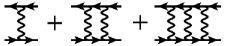
Figure 1: The diagrammatic representation of the four-vertex in the particle-hole channel in the RPA approximation. Here the interaction vertices represent the combined interaction vertex $\tilde{U}+\lambda_{3}$.

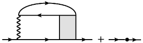
Figure 2: Diagrammatic representation of the RRPA in terms of the four-vertex and the tree-level counter-term.

To constuct an approximation to $\tilde{\Gamma}$ and $\tilde{\Sigma}$ we resort to the Renormalized Random Phase Approximation (RRPA) [17, 18, 19] which is thought to accurately describe the spin-flip excitations principally responsible for the renormalization effects at half-filling. The four-vertex is constructed by combining the two-body terms into an effective vertex $\tilde{U_{e}}=\tilde{U}+\lambda_{3}$ and resumming the particle-hole ladder of Figure 1. We thus find that

$$\tilde{U}=\frac{\tilde{U_{e}}}{1-\tilde{U_{e}}\tilde{\Pi}_{ph}(0)},$$ (16)

where $\tilde{\Pi}_{ph}(\omega)$ denotes the renormalized particle-hole propagator defined as

$$\tilde{\Pi}_{ph}(\omega)=\rmi\int_{-\infty}^{\infty}\frac{\rmd\omega^{\prime}}{2\pi}\tilde{G}^{(0)}(\omega^{\prime})\tilde{G}^{(0)}(\omega^{\prime}+\omega).$$ (17)

The self-energy is then constructed according to Figure 2 and is equal to

$$\tilde{\Sigma}(\omega)=-\rmi\int_{-\infty}^{\infty}\frac{\rmd\omega^{\prime}}{2\pi}\tilde{G}^{(0)}(\omega^{\prime}+\omega)\frac{\tilde{U_{e}}^{2}\tilde{\Pi}_{ph}(\omega^{\prime})}{1-\tilde{U_{e}}\tilde{\Pi}_{ph}(\omega^{\prime})}+\omega\lambda_{2}+\lambda_{1}.$$ (18)

We will account for the dependence of $\tilde{U}$ on $\Delta$ by considering the insertion of the infinitesimal vertex into the pair propagator and, in what constitutes only an approximation, neglecting the explicit dependence of $\tilde{U_{e}}$ on $\Delta$. We obtain then that

$$\frac{\partial\tilde{U}}{\partial\Delta}=\frac{\tilde{U_{e}}^{2}/2\pi\tilde{\Delta}^{2}}{\left(1-\tilde{\Pi}_{ph}(0)\tilde{U_{e}}\right)^{2}}.$$ (19)

Equations (14) and (19) constitute a closed system of differential equations which we will now supplmenet with boundary conditions.

4 Boundary conditions and results

In the weak-correlation regime $\Delta\rightarrow\infty$ the results of bare perturbation theory [6, 7] can be used to derive [13] the leading terms in the expressions of the renormalized parameters as functions of the bare parameters. Using the results of [20], which are based on the Bethe Ansatz, we can in fact deduce all terms order-by-order but we will not make use of this result here. Working to next-to-next-to-leading order we have that

$$\tilde{\Delta} =\Delta\left[1-\left(3-\frac{\pi^{2}}{4}\right)u^{2}+\left(105-\frac{45\pi^{2}}{4}+\frac{\pi^{4}}{16}\right)u^{4}+\ldots\right]$$

$$\tilde{U} =U\left[1-\left(\pi^{2}-9\right)u^{2}+\left(672-\frac{141\pi^{2}}{2}+\frac{\pi^{4}}{4}\right)u^{4}+\ldots\right].$$ (20)

These expressions, truncated to $\mathcal{O}(u^{2})$ in the interests of minimalism, will be used as boundary conditions to solve the system defined by (14), (19) numerically using the implementation of the Runge-Kutta-Fehlberg algorithm in the GSL library [21]. Our results are $\tilde{\Delta}(\Delta)$, $\tilde{U}(\Delta)$ are shown in Figure 3 and 4 respectively, starting from a value of $\Delta$ such that $u=0.15$. As a check we also show the renormalized parameters as determined from the NRG following the method in [14]. Additionally, we have also plotted (20) to demonstrate that the flow procedure is indeed superior to the simple inversion of the results of the bare perturbation theory.

In 3 we observe that NRG results for $\tilde{\Delta}$ are reproduced essentially exactly in weak and intermediate correlation regime. Our results start deviating from the NRG values in the neighbourhood of $u=2$ though the deviation is not amplified as we cross over to the regime of very strong correlations. Note that while in relative terms the discrepancy from the NRG is not small when $u=3.5$, the value of $\tilde{\Delta}$ has already reduced by almost three orders of magnitude. In fact, $\tilde{U}/\pi\tilde{\Delta}\approx 1$, indicating that we have already entered the Kondo regime where the universal scale $T_{K}$ emerges.

We now turn our attention to the results for $\tilde{U}/U$ shown in 4. The results in the weakly correlated regime again agree closely with the NRG though discrepancies arise as $u$ is increased sooner than in the case of $\tilde{\Delta}$. For $u\approx 1.5$ we observe a significant departure from the results of the NRG which we attribute to the somewhat crude approximation made in (19) of neglecting the dependence of $\tilde{U_{e}}$ on $\Delta$. As $u$ is increased however we find that the slope of the NRG results is reproduced and that rough agreement is maintained even when $u=3.5$.

We would like to emphasize that for both parameters the renormalization effects are very strong, with $z\approx 0.09$ when $u=3.5$. We thus consider it a success that these can be even approximately described by the flow equation method, despite the fact that a precise agreement with the results of the NRG has not been achieved. We anticipate that the accuracy of our approach can be improved by incorporating the additional corrections due to particle-particle and longitudinal scattering.

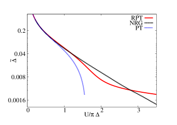
Figure 3: The renormalized hybridization $\tilde{\Delta}$ is shown as a function of $u=U/\pi\Delta$.

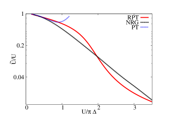
Figure 4: The ratio $\tilde{U}/U$ shown as a function of $u=U/\pi\Delta$.

5 Summary

In this article we have shown how the renormalized theory for the symmetric AIM can be used to estimate the renormalized parameters by considering infinitesimal changes to the model’s hybridization. We described how flow equations can be obtained by expressing the Lagrangian of the same bare model in terms of renormalized parameters corresponding to different $\Delta$. We also showed how an approximate flow equation for $\tilde{U}$ can be derived even in the absence of an exact Ward identity. This led to a closed system of differential equations which we then supplemented with boundary conditions derived from the results of the original perturbation theory. This was solved numerically and was found to be able to provide an estimate for the renormalized parameters in the range $u\leq 3.5$. Though our approach does not precisely reproduce the parameters it does nonetheless capture the bulk of the renormalization effects even in the strong correlation regime. By rendering the RPT independent of the NRG and self-contained we have made progress towards extending the RPT’s utility to problems that cannot be tackled by other non-perturbative methods.

References

References

- [1] P. W. Anderson. Localized magnetic states in metals. Phys. Rev., 124:41–53, Oct 1961.
- [2] Antoine Georges, Gabriel Kotliar, Werner Krauth, and Marcelo J. Rozenberg. Dynamical mean-field theory of strongly correlated fermion systems and the limit of infinite dimensions. Rev. Mod. Phys., 68:13–125, Jan 1996.
- [3] Selman Hershfield, John H. Davies, and John W. Wilkins. Probing the kondo resonance by resonant tunneling through an anderson impurity. Phys. Rev. Lett., 67:3720–3723, Dec 1991.
- [4] Yigal Meir and Ned S. Wingreen. Landauer formula for the current through an interacting electron region. Phys. Rev. Lett., 68:2512–2515, Apr 1992.
- [5] A.C. Hewson. The Kondo problem to heavy fermions. Cambridge studies in magnetism. Cambridge University Press, 1997.
- [6] Kei Yosida and Kosaku Yamada. Perturbation expansion for the anderson hamiltonian. Prog. Theor. Phys, 46(244-255):44, 1970.
- [7] Kosaku Yamada. Perturbation expansion for the anderson hamiltonian. ii. Prog. Theor. Phys, 53(970):35, 1975.
- [8] Kenneth G. Wilson. The renormalization group: Critical phenomena and the kondo problem. Rev. Mod. Phys., 47:773–840, Oct 1975.
- [9] H. R. Krishna-murthy, J. W. Wilkins, and K. G. Wilson. Renormalization-group approach to the anderson model of dilute magnetic alloys. i. static properties for the symmetric case. Phys. Rev. B, 21:1003–1043, Feb 1980.
- [10] N Andrei, K Furuya, and JH Lowenstein. Solution of the kondo problem. Reviews of modern physics, 55(2):331–402, 1983.
- [11] P B Wiegmann and A M Tsvelick. Exact solution of the anderson model: I. Journal of Physics C: Solid State Physics, 16(12):2281, 1983.
- [12] A. C. Hewson. Renormalized perturbation expansions and fermi liquid theory. Phys. Rev. Lett., 70:4007–4010, Jun 1993.
- [13] A C Hewson. Renormalized perturbation calculations for the single-impurity anderson model. Journal of Physics: Condensed Matter, 13(44):10011, 2001.
- [14] A.C. Hewson, A. Oguri, and D. Meyer. Renormalized parameters for impurity models. The European Physical Journal B - Condensed Matter and Complex Systems, 40:177–189, 2004.
- [15] K Edwards and A C Hewson. A new renormalization group approach for systems with strong electron correlation. Journal of Physics: Condensed Matter, 23(4):045601, 2011.
- [16] K. Edwards, A. C. Hewson, and V. Pandis. Perturbational scaling theory of the induced magnetization in the impurity anderson model. Phys. Rev. B, 87:165128, Apr 2013.
- [17] A C Hewson. Spin and charge dynamics in a renormalized perturbation theory. Journal of Physics: Condensed Matter, 18(5):1815, 2006.
- [18] A. C. Hewson, J. Bauer, and W. Koller. Field dependent quasiparticles in a strongly correlated local system. Phys. Rev. B, 73:045117, Jan 2006.
- [19] J. Bauer and A. C. Hewson. Field-dependent quasiparticles in a strongly correlated local system. ii. Phys. Rev. B, 76:035119, Jul 2007.
- [20] V. Zlatić and B. Horvatić. Series expansion for the symmetric anderson hamiltonian. Phys. Rev. B, 28:6904–6906, Dec 1983.
- [21] Mark Galassi, Jim Davies, James Theiler, Brian Gough, Gerard Jungman, Michael Booth, and Fabrice Rossi. Gnu Scientific Library: Reference Manual. Network Theory Ltd., February 2003.