Multi-band, Multi-epoch Observations of the Transiting Warm Jupiter WASP-80b

Abstract

WASP-80b is a warm Jupiter transiting a bright late-K/early-M dwarf, providing a good opportunity to extend the atmospheric study of hot Jupiters toward the lower temperature regime. We report multi-band, multi-epoch transit observations of WASP-80b by using three ground-based telescopes covering from optical ($g^{\prime}$, $R_{\mathrm{c}}$, and $I_{\mathrm{c}}$ bands) to near-infrared (NIR; $J$, $H$, and $K_{\mathrm{s}}$ bands) wavelengths. We observe 5 primary transits, each of which in 3 or 4 different bands simultaneously, obtaining 17 independent transit light curves. Combining them with results from previous works, we find that the observed transmission spectrum is largely consistent with both a solar abundance and thick cloud atmospheric models at 1.7$\sigma$ discrepancy level. On the other hand, we find a marginal spectral rise in optical region compared to the NIR region at the 2.9$\sigma$ level, which possibly indicates the existence of haze in the atmosphere. We simulate theoretical transmission spectra for a solar abundance but hazy atmosphere, finding that a model with equilibrium temperature of 600 K can explain the observed data well, having a discrepancy level of 1.0$\sigma$. We also search for transit timing variations, but find no timing excess larger than 50 s from a linear ephemeris. In addition, we conduct 43 day long photometric monitoring of the host star in the optical bands, finding no significant variation in the stellar brightness. Combined with the fact that no spot-crossing event is observed in the five transits, our results confirm previous findings that the host star appears quiet for spot activities, despite the indications of strong chromospheric activities.

1. Introduction

It is now well known that exoplanets have very different orbits reflecting diverse planetary origins and various migration mechanisms. To explore such planetary formation histories, unveiling their atmospheric compositions is important, because they can be affected by the environments in which they were born. For example, the relative abundances of carbon- and oxygen-bearing molecules in planetary atmospheres are closely related to the environment of surrounding disk gas (e.g., Öberg et al., 2011; Madhusudhan, 2012).

If an exoplanet has a transiting orbit, the planetary atmospheric composition can be examined by measuring transit and secondary-eclipse depths as a function of wavelength, which are referred to as transmission and emission spectroscopy, respectively. So far, several molecular features such as H₂O, CH₄, CO₂, and CO have been detected through these techniques in several hot Jupiters (e.g., Barman, 2007; Tinetti et al., 2007, 2010; Swain et al., 2008, 2009; Grillmair et al., 2008; Swain et al., 2010; Snellen et al., 2010; Wakeford et al., 2013; Deming et al., 2013), although some of the detections are still in dispute (e.g. Sing et al., 2009; Gibson et al., 2011; Swain et al., 2014). On the other hand, flat or featureless transmission spectra have also been observed in a number of exoplanets, ranging from hot Jupiters, e.g., HD 189733b, WASP-12b, HAT-P-32b, and HAT-P-1b (Pont et al., 2008; Sing et al., 2013; Gibson et al., 2013; Nikolov et al., 2014) to super-Earths/Neptunes, e.g., GJ1214b and GJ436b (Kreidberg et al., 2014; Knutson et al., 2014a), raising the possibility of the existence of floating small particles (aerosols) in their atmospheres as strong opacity sources. Such aerosols obscure or interfere with other atmospheric features (Fortney, 2005), preventing us from properly measuring the relative abundances of fundamental molecules such as H₂O, CH₄, CO₂, and CO. Therefore, understanding the nature of aerosols is crucial to explore planetary formation histories through their atmospheres.

Understanding the behaviors of aerosols is more important for cooler atmospheres. In an atmosphere with temperature below $\sim$1000 K, CH₄ becomes a major carbon carrier instead of CO. When such a CH₄-rich atmosphere is irradiated by UV fluxes, hydro-carbon haze particles (tholins) can be produced via photochemical processes. Indeed, such tholin hazes can be seen in CH₄-existing planets and satellites in our solar system (e.g., Uranus and Titan). However, few exoplanets with low-temperature atmospheres have been investigated to date. This is notable in gas giants, because transiting gas giants around late-type (low-temperature) stars are rare (e.g., Johnson et al., 2012).

In this context, a transiting Jovian planet WASP-80b was recently discovered around a nearby (60 $\pm$ 20 pc) late-K/early-M dwarf (Triaud et al., 2013). This planet has several attractive points for studying its atmosphere. First, the planet has an equilibrium temperature of $\sim$800 K or less (assuming albedo is $>$0.1), which is one of the lowest temperatures among those of transiting Jovian planets around bright ($J<$10) host stars. Second, the host star shows strong chromospheric activities (Triaud et al., 2013; Mancini et al., 2014), possibly causing active photochemical reactions in the planetary atmosphere that might produce abundant tholin particles. Last, the planet shows the second largest transit depth ($\sim$2.9 %) following Kepler-45b ($\sim$3.2%) among the known transiting planets, allowing us to measure the transit depth with relatively high precision. Therefore, WASP-80b offers a good opportunity to extend the atmospheric study toward the low-temperature regime, and test the photochemical reactions of hydro-carbons in an exoplanetary atmosphere.

Recently, Mancini et al. (2014) conducted optical-to-near-infrared simultaneous observations for a transit of WASP-80b by using the GROND instrument on the MPG/ESO 2.2 m telescope ($g^{\prime}$, $r^{\prime}$, $i^{\prime}$, $z^{\prime}$, $J$, $H$, and $K$ bands) and the 1.54 m Danish telescope ($I$ band), reporting a flat transmission spectrum within the observational uncertainties. However, because the data are also consistent with a model spectrum assuming a solar-abundance atmosphere, further observations are needed to characterize its atmosphere. Furthermore, they omitted the $H$- and $K$-band observational data in their discussion of the spectrum due to relatively poor quality, leaving large room for improvement especially in the NIR regions.

In this paper, we report multi-band, multi-epoch transit observations of WASP-80b. We observed five primary transits, each of which in three or four different bands, using three ground-based telescopes at two observatories. Such multi-band and multi-epoch observations are quite useful not only to reduce statistical uncertainties but also to check systematics in measured parameters, especially for ground-based observations which often suffer from unknown systematics and/or lack of full-transit coverages. We also report 43 day long photometric observations of the host star WASP-80 in three optical bands, to monitor its intrinsic variability. This is important because if the stellar brightness significantly varies from transit to transit due to such as star-spot appearing/vanishing, the observed transmission spectrum, or practically star-to-planet radius ratio $R_{\mathrm{p}}/R_{\mathrm{s}}$, can be biased (e.g. Pont et al., 2008).

The remainder of this paper is organized as follows. We describe our observations in Section 2. The methods of reduction and analysis of the observed data are shown in Section 3. The atmospheric properties, transit timings, and stellar variability of the WASP-80 system are discussed in Section 4. Finally, we summarize this paper in Section 5.

2. Observations

2.1. Transit Observations with IRSF/SIRIUS

We observed three primary transits of WASP-80b with the Simultaneous Infrared Imager for Unbiased Survey (SIRIUS; Nagayama et al., 2003) camera mounted on the Infrared Survey Facility (IRSF) 1.4 m telescope at the South African Astronomical Observatory on 2013 July 16, August 22, and October 7 (UT). SIRIUS has three detectors, each consisting of 1k $\times$ 1k pixels with a pixel scale of 0$\farcs$45 pixel^-1, enabling us to obtain $J$-, $H$-, and $K_{s}$-band images simultaneously with a field of view (FOV) of 7$\farcm$7 $\times$ 7$\farcm$7. During each observation, we defocused stellar images so that the FWHM of stellar point-spread function (PSF) was 14–17 pixels on July 16 and October 7, and 9.5–12 pixels on August 22, in order to improve photometric precision. In addition, we activated a software that corrects tracking errors by calculating the stellar positional shift on the newly obtained $J$-band image and feeding it back to the telescope. The exposure time was set to 10 s on July 16 and August 22, and 15 s on October 7. The weather was photometric without any thin cloud passing for the three nights. We observed full transit including pre- and post-transit parts on July 16 and October 7; however, we discarded the data before 22:47 on July 16 (UT) because of an accidental drift of the stellar position on the detector that causes uncorrectable systematic errors on photometry. The pre-transit part on August 22 was not observed due to interference with another observational program. In the lower left panel in Figures 1–3, we show the air-mass change (top) and stellar positional change along $x$ and $y$ directions on the $J$-band detector (bottom) during the respective observations. An observing log is shown in Table 1.

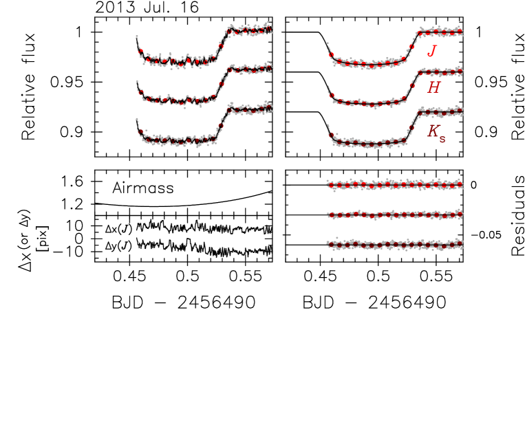
Figure 1.— (Left upper) Baseline-uncorrected transit light curves of WASP-80b observed with IRSF/SIRIUS on 2013 July 16. The $J$-, $H$-, and $K_{\mathrm{s}}$-band light curves are shown from top to bottom, where the lower two are arbitrary shifted along the vertical direction for display. The small gray points and large colored points are unbinned and 10 minute binned data, respectively. The solid lines are the best-fit transit+baseline models derived from the MCMC analysis. (Left lower) The air mass change (top), and the stellar positional changes in $x$ and $y$ directions on the $J$-band detector, where arbitrary constant values are added for clarity (bottom). (Right upper) Baseline-corrected light curves. (Right lower) Residual light curves.

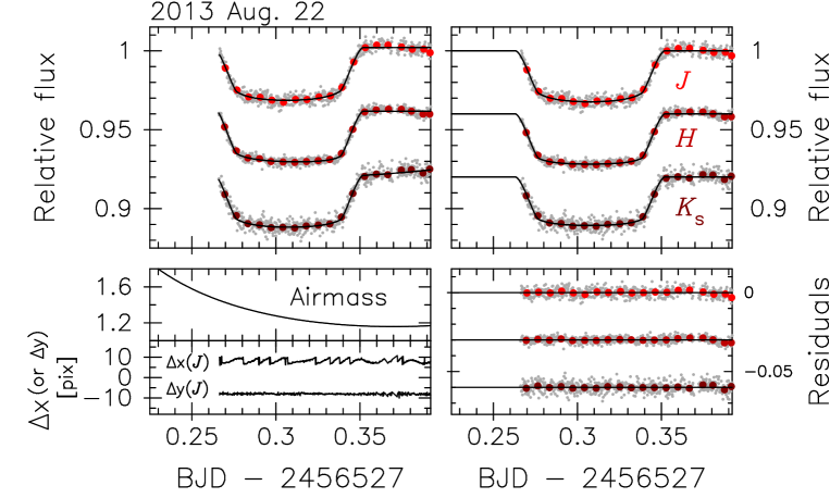
Figure 2.— Same as Figure 1, but for the data obtained on 2013 August 22.

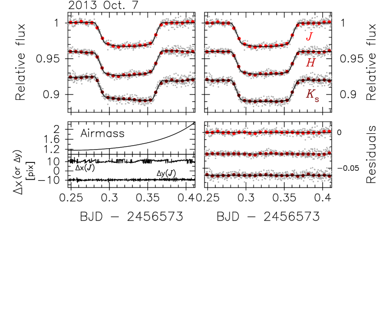
Figure 3.— Same as Figure 1, but for the data obtained on 2013 October 7.

Table 1Observing Log

Date	Telescope/	Filter	Exp. Time	$N_{\mathrm{obs}}$ a
(UT)	Instrument		(s)
2013 Jul 16	IRSF/SIRIUS	$J$	10	541
	IRSF/SIRIUS	$H$	10	537
	IRSF/SIRIUS	$K_{\mathrm{s}}$	10	539
2013 Aug 13	MITSuME 50cm	$g^{\prime}$	30	562
	MITSuME 50cm	$R_{\mathrm{c}}$	30	566
	MITSuME 50cm	$I_{\mathrm{c}}$	30	563
	OAO188cm/ISLE	$J$	45	324
2013 Aug 22	IRSF/SIRIUS	$J$	10	566
	IRSF/SIRIUS	$H$	10	576
	IRSF/SIRIUS	$K_{\mathrm{s}}$	10	582
2013 Sep 22	MITSuME 50cm	$g^{\prime}$	30	268
	MITSuME 50cm	$R_{\mathrm{c}}$	30	290
	MITSuME 50cm	$I_{\mathrm{c}}$	30	295
	OAO188cm/ISLE	$J$	45	241
2013 Oct 7	IRSF/SIRIUS	$J$	15	597
	IRSF/SIRIUS	$H$	15	597
	IRSF/SIRIUS	$K_{\mathrm{s}}$	15	603

2.2. Transit Observations with OAO188cm/ISLE and MITSuME

We observed two primary transits of WASP-80b by simultaneously using two instruments at Okayama Astrophysical Observatory (OAO) on 2013 August 13 and September 22 (UT); one is the NIR imaging and spectroscopic instrument ISLE (Yanagisawa et al., 2006, 2008) mounted on the 188 cm telescope and the other is a multi-color imager mounted on the 50 cm telescope which is one of Multicolor Imaging Telescopes for Survey and Monstrous Explosions (MITSuME; Kotani et al., 2005; Yanagisawa et al., 2010).

ISLE has a 1k $\times$ 1k HAWAII-1 array having a pixel scale of 0$\farcs$25 pixel^-1 and a FOV of 4$\farcm$5 on a side. We used $J$-band filter and set the exposure time to 45 s on both nights. We defocused stellar images so that the FWHM of stellar PSF was 23–27 pixels. In addition, we activated a hybrid auto-guiding system (Fukui et al., 2013), which consists of an off-axis auto-guiding camera to correct telescope’s tracking errors in real time, and a software that corrects a gradual drift of the origin of the auto-guiding camera with respect to the ISLE detector by calculating the shift of stellar positions on the ISLE images.

The multi-color imager mounted on the MITSuME telescope consists of three 1k $\times$ 1k CCDs, enabling us to obtain $g^{\prime}$-, $R_{\mathrm{c}}$-, and $I_{\mathrm{c}}$-band images simultaneously. Each CCD has a pixel scale of 1$\farcs$5 pixel^-1, providing a FOV of 26^′ on a side. We slightly defocused the stellar images so that the FWHM of PSF was 1.2–2.5 pixels. We also activated a software that corrects the stellar positional shift on the $I_{\mathrm{c}}$-band detector soon after each exposure. The exposure time was set to 30 s on both nights.

The weather was mostly photometric on both nights, while some thin clouds passed at the beginning of the observation on September 22, which results in large flux drops especially in the optical bands; we discarded these data from the analysis in the remainder of this paper. In the lower left panel in Figure 4 and 5, we show air-mass change (top) and stellar positional change along $x$ and $y$ directions on the ISLE (middle) and MITSuME/$I_{\mathrm{c}}$-band (bottom) detectors during the respective observations. An observing log is compiled in Table 1.

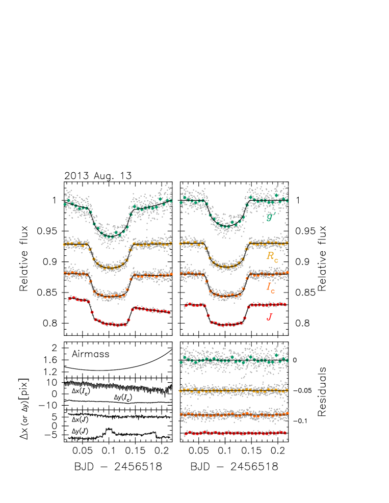
Figure 4.— (Left upper) Baseline-uncorrected transit light curves of WASP-80b observed at OAO on 2013 August 13. The $g^{\prime}$-, $R_{\mathrm{c}}$-, $I_{\mathrm{c}}$-, and $J$-band light curves are shown from top to bottom, where the lower three are arbitrary shifted along the vertical direction for display. The other meanings are the same as in Figure 1. (Left lower) The air mass change (top), and the stellar positional changes in $x$ and $y$ directions on the MITSuME/$I_{\mathrm{c}}$-band detector (middle) and those on the ISLE/$J$-band detector (bottom), where arbitral constant values are added for clarity. (Right upper) Baseline-corrected light curves. (Right lower) Residual light curves.

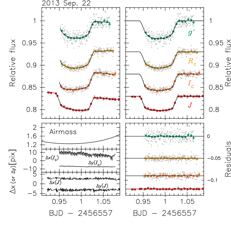
Figure 5.— Same as Figure 4, but for the data obtained on 2013 September 22.

2.3. Photometric Monitoring of Stellar Variability with MITSuME

In order to check the intrinsic variability of the host star WASP-80 around the period of our transit observations, we conducted out-of-transit observations on 14 nights spanning 43 days from 2013 August 10 to 2013 September 22, by using the 50 cm MITSuME telescope in $g^{\prime}$, $I_{\mathrm{c}}$, and $R_{\mathrm{c}}$ bands. All the settings were the same as the transit observations described in the previous section. The observations were conducted for one to two hours on each night, and in total about 1700 images were gathered for each band.

3. Analysis

3.1. Data Reduction

All the observed images are dark-subtracted and flat-fielded in a standard manner. The flat-field images are created from dozens of twilight flat images that were obtained before and after each observation for the SIRIUS and MITSuME data, and from 100 dome-flat images that were taken on each observing night for the ISLE data. After that, aperture photometry is performed for the target and several (for SIRIUS and ISLE) or dozens (for MITSuME) of bright stars spread on the reduced images, by using a customized tool with constant-aperture-radius mode (Fukui et al., 2011). The target flux is divided by the sum of the fluxes of a selected number of bright stars (comparison stars) to produce a relative light curve.

The time for each data point is assigned as the mid-time of exposure in the Barycentric Julian Day (BJD) time system based on Barycentric Dynamical Time (TDB), which is converted from Julian Day (JD) based on Coordinated Universal Time (UTC), recorded on the FITS header, via the code of Eastman et al. (2010).

3.2. Preparation of Transit Light Curves

In order to optimize the set of comparison stars and aperture radius for each instrument, filter, and transit (each data set), we produce a number of trial light curves for each data set by changing the combination of comparison stars, as well as changing the aperture radius with a step size of 0.5 pixel (for MITSuME) or 1 pixel (for others). Then, we fit the individual trial light curves with a transit-plus-baseline model to select the best light curve so that the root mean square (rms) of the residual light curve is minimum. For the light curve model, we use the following functions:

$$F = k_{0}\times 10^{-0.4\Delta m_{\mathrm{corr}}}\times F_{\mathrm{tr}},$$ (1)

$$\Delta m_{\mathrm{corr}} = \sum_{i=1}k_{i}X_{i},$$ (2)

where $F$ is the relative flux, $F_{\mathrm{tr}}$ is the transit light-curve model, $\{{\bf X}\}$ are variables for the baseline function, and $\{{\bf k}\}$ are coefficients. For the variables $\{{\bf X}\}$, we tentatively use {$t$, $z$}, where $t$ is time and $z$ is air mass. For the transit model $F_{\mathrm{tr}}$, we use the analytic formula given by Ohta et al. (2009), which is equivalent to that of Mandel & Agol (2002) when using the quadratic limb-darkening raw. The transit parameters we use are the mid-transit time $T_{\mathrm{c}}$, the planet-star radius ratio $R_{p}/R_{s}$, the semi-major axis normalized by the stellar radius $a/R_{s}$, the orbital inclination $i_{\mathrm{orb}}$, and the quadratic limb-darkening coefficients $u_{1}$ and $u_{2}$. Among these parameters, $T_{\mathrm{c}}$, $R_{p}/R_{s}$ and $u_{1}$ are let free, while $a/R_{s}$ and $i_{\mathrm{orb}}$ are fixed at the values derived from Mancini et al. (2014), namely, 12.6119 and 88.91 deg, respectively. We also fix $u_{2}$ at the theoretical values for a star with log$g$=4.5 and $T_{\mathrm{eff}}$=4100 K for respective filters, adopted from Claret et al. (2012), namely, 0.109, 0.191, 0.225, 0.223, 0.267, 0.241 for $g^{\prime}$, $R_{\mathrm{c}}$, $I_{\mathrm{c}}$, $J$, $H$, and $K_{s}$, respectively. A circular orbit, with an orbital period of $P=3.06786144$ days adopted from Mancini et al. (2014), is assumed. The individual light curves are fitted by the AMOEBA algorithm (Press et al., 1992) to find the one that gives the minimum rms value by iteratively eliminating $>$4$\sigma$ outliers. In Table 2, we summarize the number of selected comparison stars and the selected aperture radius for all data sets. The selected light curves are shown in the upper left panels in Figures 1–5, where 10 minute binned data are also shown as a visual guide. We note that there exists a fainter neighboring star ($\Delta B$=2.8 and $\Delta K_{\mathrm{s}}$=4.0) that is separated from WASP-80 by 8$\farcs$9; we confirm that with the selected aperture radii the flux contamination from the fainter star is negligible for all the data sets.

3.3. Selection of Baseline Models

After preparing the light curves, we select the best-describing baseline model, i.e., which variables should be included in $\{{\bf X}\}$ in Equation (2), for each light curve. To do so, we first fit each light curve with Equations (1) and (2), letting $T_{\mathrm{c}}$, $R_{p}/R_{s}$, $u_{1}$, and $a/R_{\mathrm{s}}$ be free while fixing others, by changing the set of variables $\{{\bf X}\}$. The set of variables are chosen from $t$, $z$, $t^{2}$, $\Delta x$, and $\Delta y$, where $\Delta x$ and $\Delta y$ are the relative stellar displacement along the $x$ and $y$ directions, respectively, on the detectors. Next, we evaluate the Bayesian information criteria (BIC; Schwarz, 1978) for each baseline model; the BIC value is given by BIC=$\chi^{2}+k\ln N$, where $k$ is the number of free parameters and $N$ is the number of data points. Finally, we select the best baseline model such that the BIC value is minimum.

This procedure works well for all the light curves except for the $J$- and $H$-band light curves obtained on 2013 August 22. For these two light curves, we find that the fittings with the minimum-BIC models, namely $\{{\bf X}\}$={$t,t^{2}$} for both, derive inconsistent $a/R_{\mathrm{s}}$ values with that derived from Mancini et al. (2014), although for all the other light curves the comparable fittings derive consistent $a/R_{\mathrm{s}}$ values, largely within their uncertainties (see Figure 6). The two exceptional light curves lack a pre-transit part; in such a case, incorrect baseline models can incidentally fit the data well. If this is the case, the derived $R_{\mathrm{p}}/R_{\mathrm{s}}$ value, which is what we want to measure, could be shifted from the true value. In fact, the respective $R_{\mathrm{p}}/R_{\mathrm{s}}$ values for the $J$- and $H$-band light curves on August 22 are significantly larger than those for the light curves from the same band on October 7 (see the corresponding panels in Figure 6), which depict both before and after the transit. For the two exceptions, we alternatively find that a simpler baseline model of $\{{\bf X}\}$ = {$z$} can fit them giving consistent $a/R_{\mathrm{s}}$ values with those from Mancini et al. as well as consistent $R_{\mathrm{p}}/R_{\mathrm{s}}$ values with the light curves from the same band on October 7 (denoted as open circles in Figure 6), while the BIC differences between $\{{\bf X}\}$ = {$z$} and {$t,t^{2}$} for the $J$- and $H$-band light curves are 18.8 and 34.1, respectively. For the above reasons, we choose $\{{\bf X}\}$ = {$z$} as the best baseline model for these two light curves. We note that it is not likely that $a/R_{\mathrm{s}}$ and $R_{\mathrm{p}}/R_{\mathrm{s}}$ have changed over time, because fitting to the $K_{\mathrm{s}}$-band light curve on the same night with the minimum-BIC model gives a $a/R_{\mathrm{s}}$ value that is consistent with that of Mancini et al. In Table 2, we summarize the selected sets of variables {X} for the respective light curves.

We also note that even for the other light curves, there can be several baseline models that give BIC values similar to the minimum one, potentially causing systematic errors on $R_{\mathrm{p}}/R_{\mathrm{s}}$ depending on which baseline model we select. To see the impact of this possibility, we also plot in Figure 6 the $R_{\mathrm{p}}/R_{\mathrm{s}}$ and $a/R_{\mathrm{s}}$ values for the baseline models that give the BIC difference with respect to the minimum-BIC model ($\Delta$BIC) of less than five. As a result, the $R_{\mathrm{p}}/R_{\mathrm{s}}$ and $a/R_{\mathrm{s}}$ values for similar-BIC models (filled circle, triangle, and square are for the minimum, second-, and third-minimum BIC models, respectively) are close to each other compared to their uncertainties, implying that the systematics on $R_{\mathrm{p}}/R_{\mathrm{s}}$ due to different baseline models are small.

After the baseline-selection process, we rescale the flux uncertainties in each light curve such that the reduced $\chi^{2}$ of the transit-plus-baseline-model fit becomes unity. In addition, we further rescale these uncertainties by the so-called $\beta$ factor (Winn et al., 2008) taking red noises into account. The $\beta$ factor is defined as $\sigma_{N,\mathrm{obs}}$/$\sigma_{N,\mathrm{exp}}$, where $\sigma_{\mathrm{N,obs}}$ is the standard deviation of the residual light curve binned by $N$ data points into $M$ bins, and $\sigma_{N,\mathrm{exp}}\equiv\sigma_{1}\sqrt{M/N(M-1)}$ is the expected standard deviation for the binned residual light curve assuming that the unbinned residuals with the standard deviation of $\sigma_{1}$ are dispersed in a Gaussian distribution. We take the median value of $\beta$ calculated for $N=$ 4 to 15 for each light curve. The calculated $\beta$ values are summarized in Table 2.

Table 2Summary of Light Curve Preparation

Instrument	Obs. Date	Filter	$N_{\mathrm{comp}}$ a	$R_{\mathrm{ap}}$ b	$\{{\bf X}\}$	RMS	$\beta$
	(UT)			(pixel)		(%)
SIRIUS	2013 Jul 16	$J$	3	12.0	$t$, $\Delta x$, $\Delta y$	0.194	1.24
		$H$	3	14.0	$t$, $\Delta x$, $\Delta y$	0.145	1.58
		$K_{\mathrm{s}}$	4	12.0	$t$, $\Delta x$, $\Delta y$	0.200	1.33
	2013 Aug 22	$J$	3	9.0	$z$	0.251	1.36
		$H$	3	9.0	$z$	0.177	1.68
		$K_{\mathrm{s}}$	2	9.0	$t$, $z$	0.298	1.13
	2013 Oct 7	$J$	3	16.0	$t$	0.270	1.06
		$H$	2	16.0	$t$, $z$, $t^{2}$	0.265	1.17
		$K_{\mathrm{s}}$	3	14.0	$t$, $z$, $t^{2}$	0.329	1.01
ISLE	2013 Aug 13	$J$	1	20.0	$t$	0.164	1.35
	2013 Sep 22	$J$	1	21.0	$t$, $z$	0.177	1.28
MITSuME	2013 Aug 13	$g^{\prime}$	8	2.5	$t$, $t^{2}$	1.05	1.02
		$R_{\mathrm{c}}$	6	4.0	$z$	0.477	1.00
		$I_{\mathrm{c}}$	9	3.5	$t$	0.491	1.01
	2013 Sep 22	$g^{\prime}$	8	3.0	$t$	0.855	1.00
		$R_{\mathrm{c}}$	6	4.0	$z$	0.417	1.12
		$I_{\mathrm{c}}$	9	3.5	$t$, $t^{2}$	0.404	1.08

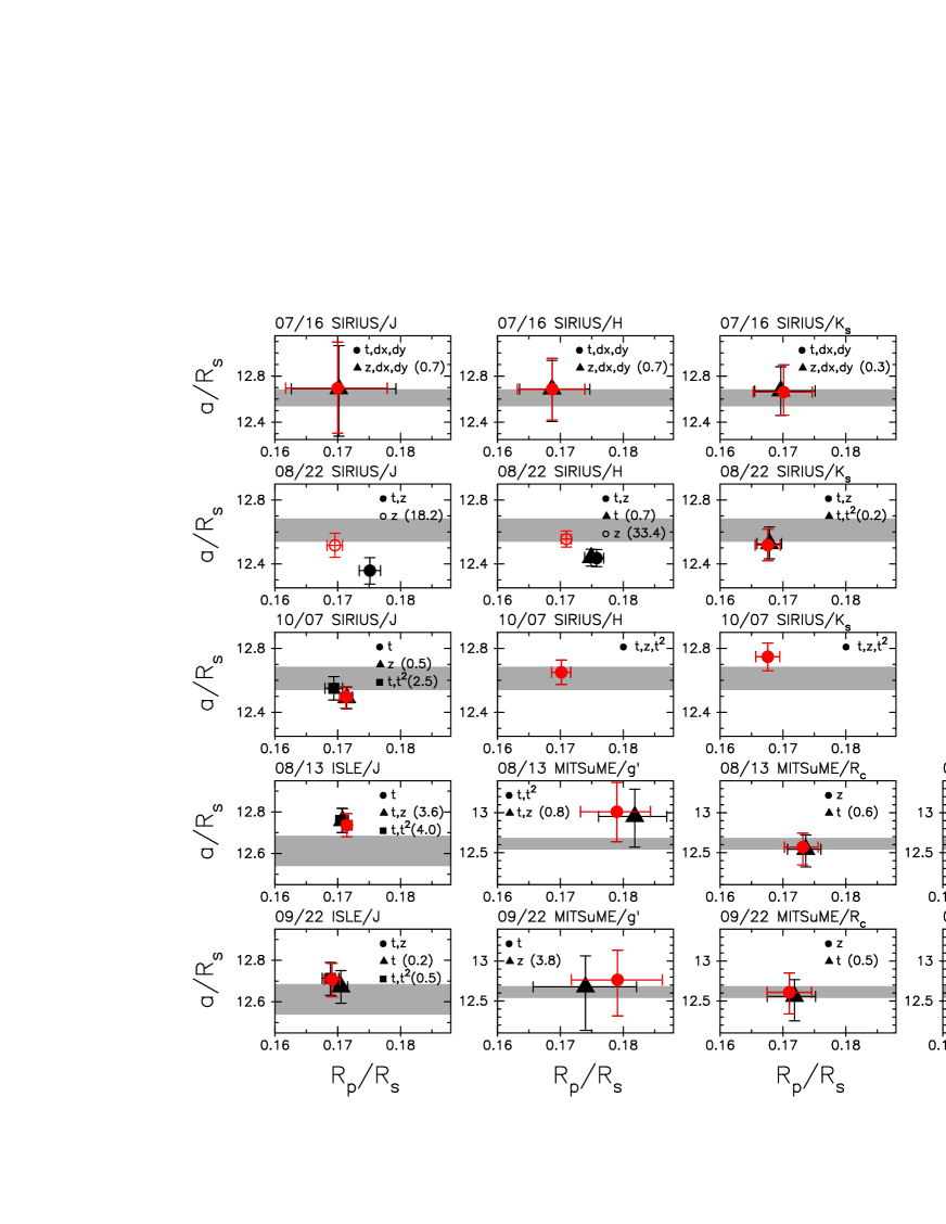
Figure 6.— Comparison of $R_{\mathrm{p}}/R_{\mathrm{s}}$ and $a/R_{\mathrm{s}}$ derived by the AMOEBA fitting for each light curve using different baseline models. The results for each light curve are shown in each panel, on top of which the observing month/day and instrument/filter are indicated. The filled circle, triangle, and square denote the values derived by using the baseline models that give the minimum, second minimum, and third minimum BIC values, respectively. The number in parenthesis in the legend indicates $\Delta$BIC with respect to the minimum BIC value. Note that only the plots giving $\Delta$BIC$<$5 are shown in this figure, except for the panels for SIRIUS/$J$ and $H$ on August 22, where the values derived from {X} = {$t$} are additionally shown as open circles. The gray belt indicates the 1$\sigma$ credible region of $a/R_{\mathrm{s}}$ derived by Mancini et al. (2014). Our choices for the best-describing baseline models are indicated by red color.

3.4. MCMC Analysis

To properly derive the $R_{\mathrm{p}}/R_{\mathrm{s}}$ values and their uncertainties for the respective data sets, we perform the Markov Chain Monte Carlo (MCMC) analysis for each transit by using a customized code (Narita et al., 2007, 2013). In this analysis, all the light curves involved in one transit are analyzed simultaneously, treating $i_{\mathrm{orb}}$, $a/R_{\mathrm{s}}$, and $T_{\mathrm{c}}$ as common parameters, whereas $R_{\mathrm{p}}/R_{\mathrm{s}}$, $u_{1}$, $u_{2}$, and $\{{\bf k}\}$ are treated as independent parameters for the respective light curves. Here, $\{{\bf k}\}$ are the coefficients corresponding to the variables {X} selected in the previous section. In the same way as in Section 3.2, we fix $i_{\mathrm{orb}}$ and $a/R_{\mathrm{s}}$ at the values from Mancini et al. (2014), and fix $u_{2}$ at the theoretical values for the respective filters; we let the other adjustable parameters be free. The reason for fixing the $i_{\mathrm{orb}}$ and $a/R_{\mathrm{s}}$ values to those of Mancini et al. is that these parameters are correlated with $R_{\mathrm{p}}$/$R_{\mathrm{s}}$, and varying them would cause systematic offset on measured $R_{\mathrm{p}}$/$R_{\mathrm{s}}$, which is what we aim to compare between different bands among the data including the ones from Mancini et al. (see Section 4.1).

We start the MCMC procedure with the best-fit parameters determined by the AMOEBA algorithm, using their 1$\sigma$ uncertainties as the widths of Gaussian jump functions for updating MCMC steps. We perform 10 sequential MCMC runs with 10⁶ chained steps in each run, updating the best-fit parameters and their 1$\sigma$ uncertainties. To wait for convergence, we discard the first five MCMC runs. The final median values and 1$\sigma$ uncertainties of the respective parameters are calculated from the merged posterior-probability distributions from the last five MCMC runs.

The resultant parameters are summarized in Table 3. The final light curve models are displayed as solid lines in the upper left panels in Figures 1–5, as well as the baseline-corrected light curves and residual light curves are shown in the upper right and lower right panels, respectively, in the same figures. We note that no apparent spot-crossing event is seen in any of the five transits.

Table 3MCMC Results^a

Parameter			Value
	2013 Jul 16	2013 Aug 13	2013 Aug 22	2013 Sep 22	2013 Oct 7	Mancini et al. (2014)
$T_{\mathrm{c}}$	6490.492507	6518.10335	6527.30758	6557.98585	6573.32468	…
[BJDTDB-2450000]	$\pm$ 0.000091	$\pm$ 0.00012	$\pm$ 0.00016	$\pm$ 0.00018	$\pm$ 0.000088
$u_{1}$ ($g^{\prime}$)	…	0.842 $\pm$ 0.087	…	0.642 ${}^{0.095}_{-0.097}$	…	…
$u_{1}$ ($R_{\mathrm{c}}$)	…	0.624 ${}^{0.042}_{-0.043}$	…	0.551 ${}^{0.056}_{-0.059}$	…	…
$u_{1}$ ($I_{\mathrm{c}}$)	…	0.407 ${}^{0.048}_{-0.050}$	…	0.353 ${}^{0.052}_{-0.054}$	…	…
$u_{1}$ ($J$)	0.270 $\pm$ 0.026	0.254 $\pm$ 0.032	0.265 ${}^{0.035}_{-0.037}$	0.258 ${}^{0.038}_{-0.040}$	0.204 $\pm$ 0.027	…
$u_{1}$ ($H$)	0.213 $\pm$ 0.023	…	0.126 ${}^{0.033}_{-0.031}$	…	0.133 ${}^{0.033}_{-0.038}$	…
$u_{1}$ ($K_{\mathrm{s}}$)	0.153 $\pm$ 0.029	…	0.159 $\pm$ 0.038	…	0.048 ${}^{0.048}_{-0.053}$	…
$R_{\mathrm{p}}/R_{\mathrm{s}}$ ($g^{\prime}$)	…	0.1743 ${}^{0.0045}_{-0.0047}$	…	0.1787 $\pm$ 0.0064	…	0.17033 $\pm$ 0.00217
$R_{\mathrm{p}}/R_{\mathrm{s}}$ ($R_{\mathrm{c}}$)	…	0.1736 $\pm$ 0.0017	…	0.1711 ${}^{0.0040}_{-0.0037}$	…	0.17041 $\pm$ 0.00175
$R_{\mathrm{p}}/R_{\mathrm{s}}$ ($I_{\mathrm{c}}$)	…	0.1741 $\pm$ 0.0015	…	0.1778 $\pm$ 0.0039	…	0.17183 $\pm$ 0.00161
$R_{\mathrm{p}}/R_{\mathrm{s}}$ ($J$)	0.1697 $\pm$ 0.0015	0.1704 $\pm$ 0.00092	0.1690 $\pm$ 0.0014	0.1686 $\pm$ 0.0016	0.17234 ${}^{0.00089}_{-0.00081}$	0.1695 $\pm$ 0.0028
$R_{\mathrm{p}}/R_{\mathrm{s}}$ ($H$)	0.1688 $\pm$ 0.0014	…	0.1709 $\pm$ 0.0012	…	0.1702 $\pm$ 0.0017	…
$R_{\mathrm{p}}/R_{\mathrm{s}}$ ($K_{\mathrm{s}}$)	0.1708 $\pm$ 0.0016	…	0.1672 $\pm$ 0.0022	…	0.1679 $\pm$ 0.0023	…

3.5. Photometric Monitoring Data

For the 43 day long photometric monitoring data gathered by the MITSuME telescope, we perform aperture photometry in the same way as in Sections 3.1 and 3.2. After eliminating the data points fallen in any transit events, we correct the systematics on the respective light curves by fitting them with Equations (1) and (2) fixing $F_{\mathrm{tr}}$=1 and using $\{{\bf X}\}$={$z$, $\Delta x$, $\Delta y$}. The resultant light curves with nightly binned data points are shown in Figure 7, in which the error bars are calculated as rms of the unbinned data on each night divided by the square of the number of data points.

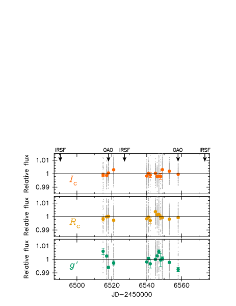
Figure 7.— Forty-three-day-long light curves of WASP-80 observed with the MITSuME telescope in $I_{\mathrm{c}}$, $R_{\mathrm{c}}$, and $g^{\prime}$ bands (top, middle, and bottom panels, respectively). The gray dots are unbinned data points excluding those that fall in any transits, whereas the large points indicate nightly binned data. The error bars are calculated as RMS of nightly unbinned data divided by square of the number of data points. The nights when the transit observations were conducted at IRSF and OAO are indicated as arrows in the top panel.

4. Discussion

4.1. Atmospheric Properties

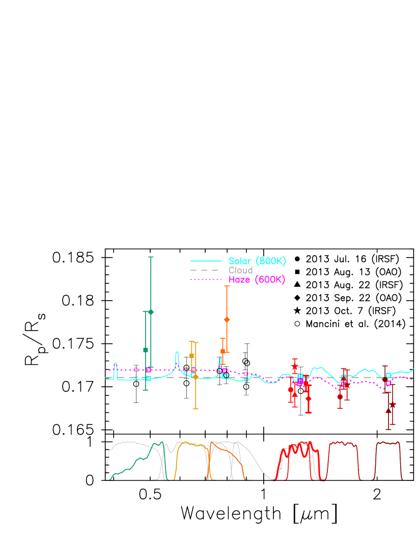
Figure 8.— (Top) Observed and theoretical transmission spectra of WASP-80b. The $R_{\mathrm{p}}/R_{\mathrm{s}}$ values obtained in this work are indicated as filled marks, where different marks are for the data obtained on different nights as indicated at the upper right in the panel. The $J$-band data from ISLE are indicated as bold lines for ease of recognizing. The open circles indicate the data from Mancini et al. (2014), which include re-analysis of the data presented in Triaud et al. (2013). Data points are slightly shifted in the horizontal direction for display when there are multiple observations at one band pass. The solid, dashed, and dotted lines show theoretical spectra for solar-abundance (800K), cloudy, and hazy (600K) atmospheres, respectively (see text for details). Note the theoretical spectra shown are smoothed for clarity. The open squares indicate the integrals of the theoretical spectra for the respective band passes. (Bottom) Transmission curves for the respective filters, where the bold, normal, and thin lines are for the ISLE/$J$-band filter, the other filters used in this work, and those used in Mancini et al. (2014), respectively.

In this section, we discuss the dependence of $R_{\mathrm{p}}/R_{\mathrm{s}}$ on wavelength that could arise from the atmospheric properties of WASP-80b. In Figure 8, we plot the observed $R_{\mathrm{p}}/R_{\mathrm{s}}$ values derived in Section 3.4 as a function of wavelength, along with those derived by Mancini et al. (2014). At each band, the measured values from different transits are consistent with each other within 2$\sigma$ uncertainties. Especially in the $J$ band, we have now a total of six observations of $R_{\mathrm{p}}/R_{\mathrm{s}}$ including the one from Mancini et al. (2014), and they are mostly consistent with each other, indicating the correctness of our methodology and the smallness of systematics. We note that the effect of stellar intrinsic variability on measured $R_{\mathrm{p}}/R_{\mathrm{s}}$ is negligible, as will be discussed in Section 4.3.

In order to search for atmospheric features in the observed $R_{\mathrm{p}}/R_{\mathrm{s}}$ spectrum, we first compare the overall observed data with two possible model spectra; one is from an atmospheric model with the solar abundances and the other is from an atmospheric model with opaque clouds. For the former model, we simulate the model spectrum assuming a solar abundance atmosphere and a temperature of 800 K, which corresponds to the equilibrium temperature with albedo of 0.1 (Triaud et al., 2013), as described in the Appendix; for the latter model, we approximate it simply as a flat line assuming that the atmosphere is thoroughly opaque in the wavelength range from optical to NIR. Note that our motivations for comparing with the cloudy model come from the fact that flat transmission spectra compatible with the presence of thick cloud layers have been recently observed for several other low-temperature exoplanets such as GJ1214b (Kreidberg et al., 2014) and GJ436b (Knutson et al., 2014b), as well as the fact that Mancini et al. (2014) reported that their observed spectrum of WASP-80b is consistent with a flat line. We then fit the two model spectra to the data; for both cases, the number of free parameters is one: the radius of planetary disk that blocks the incident stellar radiation completely, $R_{0}$.

In the fitting process, we create a theoretical $R_{\mathrm{p}}/R_{\mathrm{s}}$ spectrum for each $R_{0}$ using Equation (A2) and the fixed $R_{\mathrm{s}}$ value of 0.63 $R_{\odot}$ (Triaud et al., 2013), and integrate the spectrum over each filter’s pass band to compare it with the observational data. The best-fitted models for the solar abundance atmosphere and the cloudy atmosphere are shown, respectively, by the solid cyan and dashed gray lines in Figure 8. As a result, we find that the solar abundance and cloudy models give the minimum-$\chi^{2}$ values of 35.4 and 34.7, respectively, for the degrees of freedom (dof) of 25. These values indicate that the two models are both largely consistent with the data at the discrepancy level of 1.7$\sigma$. When we discard the MITSuME data, which were obtained with a relatively small-aperture telescope and might contain relatively large unknown systematics, the solar abundance and cloudy models fit the remaining data with $\chi^{2}$/dof=24.3/19 and 22.7/19, respectively, reducing the discrepancy levels to 1.3 and 1.1$\sigma$. Therefore, we cannot rule out these two models from the current observational data.

On the other hand, we also find that the observed $R_{\mathrm{p}}/R_{\mathrm{s}}$ in the optical region is marginally larger than that in the NIR region; the weighted mean of the observed $R_{\mathrm{p}}/R_{\mathrm{s}}$ in the optical ($\lambda<1\mu$m) and NIR ($\lambda>1\mu$m) regions are 0.17193 $\pm$ 0.00041 and 0.17029 $\pm$ 0.00039, respectively, having a 2.9-$\sigma$ discrepancy. As discussed in Section 1, because the equilibrium temperature of WASP-80b is about 800 K or less, photochemically produced hydro-carbon haze like tholin may exist in the atmosphere (e.g., Fortney et al., 2013). If so, the observed spectral rise in the optical region could be explained by the existence of tholin haze in the planetary atmosphere.

Motivated by this possibility, we model the transmission spectrum of a hazy atmosphere with the solar abundances and compare it with the observed data. The haze layer is characterized by four parameters that include the particle size $a_{\mathrm{haze}}$, the number density $n_{\mathrm{haze}}$, and the pressures at the top and bottom of the haze layer, which are denoted by $P_{\mathrm{top}}$ and $P_{\mathrm{bot}}$, respectively. Values of $P_{\mathrm{top}}$ and $P_{\mathrm{bot}}$ are chosen as described in the Appendix; in the case of GJ1214b, the method of choice is confirmed to yield values of $P_{\mathrm{top}}$ and $P_{\mathrm{bot}}$ that are consistent with the result from Morley et al. (2013). We assume $a_{\mathrm{haze}}=0.04$ $\mu$m, which is the typical size of haze particles in Titan’s atmosphere (Tomasko et al., 2009). We then search for the best-fit hazy model by changing $n_{\mathrm{haze}}$ every one order of magnitude from 10 to $1\times 10^{6}$ cm^-3, as well as letting $R_{0}$ be free. As a result, we find that $n_{\mathrm{haze}}=1\times 10^{4}$ cm^-3 gives a minimum-$\chi^{2}$ value of 29.3 with dof = 24 (in this case, the number of free parameters is two) for temperature of 800 K, which means that the discrepancy level is 1.3$\sigma$. A comparable fit to the data without the MITSuME data gives $\chi^{2}$/dof = 22.7/18, or 0.99$\sigma$. These values are slightly better than those for the above two models of the haze-free solar-abundance atmosphere and the cloudy atmosphere.

In reality, however, we may have to consider temperature lower than 800 K. The 800 K corresponds to the globally averaged equilibrium temperature of WASP-80b with an albedo of 0.1. Since WASP-80b is likely to be tidally locked, the limb of the planetary disk that we observe may be much cooler than 800 K, provided the atmospheric heat redistribution is inefficient. Also, the high-altitude haze may block incident stellar flux from reaching the deep atmosphere. Thus, we consider 600 K, as an example of a moderately warm atmosphere to simulate the transmission spectrum which is shown by the dotted magenta line in Figure 8. In this case, the best-fit model (with $n_{\mathrm{haze}}=1\times 10^{4}$ cm^-3) results in a $\chi^{2}$/dof of 26.8/24, giving a discrepancy level of only 1.0$\sigma$. These statistical values decrease to $\chi^{2}$/dof=19.5/18 and 0.92$\sigma$ for the case without the MITSuME data. These results indicate that the hazy atmosphere model with temperature of 600 K is rather consistent with the observed data, relative to the above three models. In contrast, we also find that the haze-free solar abundance atmosphere of 600 K yields a large $\chi^{2}$/dof of 44.2/25 and 29.7/19 for the data with and without the MITSuME data, respectively. In Table 4, we summarize the statistical results of the model fittings discussed above.

A more extensive search for the best-fit model is beyond the scope of this study because the observed data have uncertainties that are too large and wavelength resolutions that are too low. Also, we need more detailed treatment concerning the role of haze on the atmospheric temperature and the heat redistribution in the atmosphere, which will be left to future studies. Nevertheless, we confirm that at least one atmospheric model with haze can explain the observed data well. Thus, the relatively large $R_{\mathrm{p}}/R_{\mathrm{s}}$ in the optical region detected by our observation has raised another possibility of the presence of haze in the atmosphere. Higher-precision and higher-wavelength-resolution observations are desired to further shed light on this possibility.

Table 4Statistical Results of Model Fitting to the Transmission Spectrum

	Solar	Cloud	Haze	Haze	Solar
	(800 K)		(800 K)	(600 K)	(600 K)
All Data
$\chi^{2}$/dof	35.4/25	34.7/25	29.3/24	26.8/24	44.2/25
Discrepancy [$\sigma$]	1.7	1.7	1.3	1.0	2.7
w/o MITSuME Data
$\chi^{2}$/dof	24.3/19	22.7/19	20.2/18	19.5/18	29.7/19
Discrepancy [$\sigma$]	1.3	1.1	0.99	0.92	1.9

4.2. Transit Timings

Due to the multi-epoch observations, we are able to refine the transit ephemeris as well as search for transit timing variations (TTVs) that would be caused by additional perturbing planets (e.g., Holman et al., 2010). The latter is particularly of interest because warm Jupiters may have higher probability of having TTV-causing neighboring planets compared to hot Jupiters, most of which are known to be solitary (e.g., Steffen et al., 2012).

Using the mid-transit times of the five transits measured in Section 3.4 as well as those from the previous works, we refine the transit ephemeris of WASP-80b as $T_{\mathrm{c}}\ \mathrm{(BJD_{TDB})}=$ 2456125.417574 (86) + 3.06785952 (77) $\times E$, where $E$ is the relative transit epoch and the numbers in parentheses indicate the uncertainties written to the last two significant digits. The residuals of the observed transit timings from the above ephemeris are shown in Figure 9. The $\chi^{2}$ value for the linear fit is 59.0 for the degrees of freedom of 11, indicating that a liner function does not fit the data well. This in principle could be due to perturbations from an additional object in the planetary system, however, it could also be due to small-number statistics and/or unknown systematics as well (e.g. Maciejewski et al., 2013; Barros et al., 2013; Southworth et al., 2012; Hoyer et al., 2012). In addition, we cannot see any plausible periodicity nor large amplitude exceeding $\sim$50 s that are usually seen in the detection cases (e.g. Mazeh et al., 2013). Therefore, we do not claim a detection of TTVs due to a third body at this time.

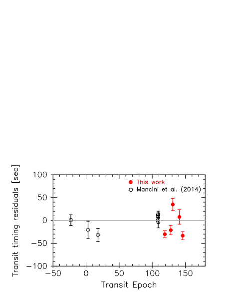
Figure 9.— Residuals of the observed mid-transit times from the liner ephemeris calculated by fitting all the data shown here. The latest five data points are from this work, and others are from Mancini et al. (2014) including the re-analysis data of the light curves presented in Triaud et al. (2013).

4.3. Stellar Variability

To check for the existence/absence of stellar intrinsic variability that causes systematic offsets on the observed $R_{\mathrm{p}}/R_{\mathrm{s}}$, we investigate the 43 day long light curves created in Section 3.5. The $\chi^{2}$ values of the 14 nightly binned data with respect to a constant fit are 212.7, 181.8, and 137.4 for $g^{\prime}$, $R_{\mathrm{c}}$, and $I_{\mathrm{c}}$ bands, respectively, suggesting that the host star’s brightness could significantly vary over time. However, the data points in different bands are not correlated each other, with the correlation coefficients between $I_{\mathrm{c}}$ and $R_{\mathrm{c}}$, $R_{\mathrm{c}}$ and $g^{\prime}$, and $g^{\prime}$ and $I_{\mathrm{c}}$ are $-0.26$, 0.29, $-0.32$, respectively. This fact indicates that the observed dispersions are due to systematics rater than astrophysical origin. In addition, no periodic variation or linear trend can be seen in any of the three light curves. Therefore, we do not detect any star-spot-induced periodic variability with the semi-amplitude larger than 0.25%, 0.3%, and 0.7% for $I_{\mathrm{c}}$, $R_{\mathrm{c}}$, and $g^{\prime}$ bands, respectively, during the observed period range of 43 days. Even if the observed dispersions were of astrophysical origins, the maximum variability of 0.7% in the $g^{\prime}$ band would change the observed $R_{\mathrm{p}}/R_{\mathrm{s}}$ values by only 0.07%, or 0.0001 in units of $R_{\mathrm{p}}/R_{\mathrm{s}}$, which is negligible compared to the uncertainties of $R_{\mathrm{p}}/R_{\mathrm{s}}$.

The non-detection of significant stellar variability is in line with the report of Triaud et al. (2013), who did not detect $>$1 mmag rotational variability from wide-band ($V$+$R$) photometric data of the WASP transit survey as well as from multi-epoch observations with a 60 cm telescope. We therefore confirm from the multi-band observations that the host star WASP-80 does not show spot-induced large ($>$ a few mmag) periodic variations. In addition, so far no spot-crossing event has been observed during any of the transits observed in this work or in previous works (nine transits in total), implying that there are not many or large spots distributed on the stellar surface. On the other hand, Triaud et al. (2013) pointed out that the star could be young because of its high projected stellar rotational velocity ($v\mathrm{sin}i_{\mathrm{s}}=3.55\pm 0.33$ km s^-1), depletion of lithium, and the presence of Ca $H$+$K$ emission, although there is also counter-evidence that the galactic dynamical velocities are low. In addition, Mancini et al. (2014) detected strong Ca $H$+$K$ emission lines, indicating that the star has strong magnetic activity. If the star is truly young and active, the star would be expected to be heavily spotted. If so, a possible scenario would be that either many small spots are widely distributed on the stellar surface (Mancini et al., 2014), or that the stellar inclination $i_{\mathrm{s}}$ is very small such that the polar region of the stellar surface is always facing us. The latter idea is particularly consistent with the fact that the projected spin-orbit angle $\beta$ was measured as a significantly non-zero value ($\pm 75^{\circ}\pm 4$), assuming $V\mathrm{sin}i_{\mathrm{s}}$ = $v\mathrm{sin}i_{\mathrm{s}}$, where $V\mathrm{sin}i_{\mathrm{s}}$ and $v\mathrm{sin}i_{\mathrm{s}}$ are the projected stellar-rotation velocities measured from the Rossiter-McLaughlin effect and spectral equivalent width, respectively (Triaud et al., 2013). In this case, the star should be rotating very fast, possibly less than a few days. Photometric monitoring of the star with much higher precision may help to measure the rotational period and test this possibility.

5. Summary

In this paper, we report multi-color, multi-epoch observations of the transiting warm Jupiter WASP-80b, which is suitable for studying an exoplanetary atmosphere with low temperature. We observed five primary transits of this planet using three instruments and seven different filters. Consequently, we obtained 17 independent transit light curves in six colors covering from optical to near infrared (NIR) wavelength regions. We compare the observed $R_{\mathrm{p}}/R_{\mathrm{s}}$ values including those from previous works with two model spectra, one is from a solar-abundance atmospheric model and the other is from a thick cloud one. As a result, we find that the observed data are largely consistent with both the two models at 1.7$\sigma$. Therefore, we cannot rule out these two models from the current observations.

On the other hand, we also find that the observed $R_{\mathrm{p}}/R_{\mathrm{s}}$ in optical is marginally larger than that in NIR at 2.9$\sigma$ significance, possibly indicating the existence of haze in the planetary atmosphere. We compare the data with theoretical spectra for a solar abundance but hazy atmosphere, and find that a model with the equilibrium temperature of 600K fits the data at 1.0$\sigma$, indicating that the hazy atmospheric model can explain the observed data well. To confirm or reject this possibility, further higher-precision and higher-spectral-resolution observations are required.

We also search for transit timing variations from totally 13 timing data (9 transits) from this work and previous work. As a result, we do not find any periodic timing variation nor timing excess larger than 50 s from a linear ephemeris, meaning that there is no considerable sign of additional neighboring planet at this time.

In addition, we conducted 43 day long photometric monitoring of the host star in $g^{\prime}$, $R_{\mathrm{c}}$, and $I_{\mathrm{c}}$ bands, resulting in a non-detection of significant brightness variations. Combining with the fact that no spot-crossing event is observed in the five transits, we confirm the findings of Triaud et al. (2013) and Mancini et al. (2014) that the host star appears quiet for spot activities despite indications of strong chromospheric activities. This odd consequence could be explained if the host star has a polar-on orbit. This possibility can be tested by measuring the stellar rotational period by monitoring the stellar brightness with much higher precision.

Appendix A Outline of Transmission Spectrum Modeling

The theoretical value of the transit radius at wavelength $\lambda$, $R_{\mathrm{p,th}}(\lambda)$, is calculated as

$$\left[\frac{R_{\mathrm{p,th}}(\lambda)}{R_{\mathrm{s}}}\right]^{2}=\frac{1}{\pi R_{\mathrm{s}}^{2}}\int_{0}^{R_{\mathrm{s}}}\left\{1-e^{-\tau(r,\lambda)}\right\}\cdot 2\pi rdr,$$ (A1)

where $R_{\mathrm{s}}$ is the host star’s radius, $r$ is the planetocentric distance, and $\tau$ is the chord optical thickness (see e.g. Kurosaki et al., 2014). We assume that the planetary disk of radius $R_{0}$ blocks the incident stellar radiation completely, which means

$$\left\{R_{\mathrm{p,th}}(\lambda)\right\}^{2}=R_{0}^{2}+\int_{R_{0}^{2}}^{R_{\mathrm{s}}^{2}}\left\{1-e^{-\tau(r,\lambda)}\right\}dr^{2}.$$ (A2)

In this study, we define $R_{0}$ as the planetocentric distance at which the atmospheric pressure is 10 bar. Since the pressure profile in the atmosphere is unknown in advance, we treat $R_{0}$ as a free parameter while searching for the best-fit model by $\chi^{2}$ analysis. The atmosphere is assumed to be in hydrostatic equilibrium and isothermal for simplicity; $R_{\mathrm{p,th}}$ is known to be less sensitive to atmospheric pressure-temperature profiles (Miller-Ricci & Fortney, 2010; Howe & Burrows, 2012). We also assume that the element abundances are radially constant and calculate chemical-equilibrium molar fractions of molecules at each altitude with the Gibbs free energy data from NIST-JANAF Thermochemical Tables (Chase, 1998). We determine the element abundance ratios of the solar abundance atmosphere from Lodders (2003).

As for the sources of radiative extinction, we consider line absorption by H₂, H₂O, CH₄, CO, CO₂, NH₃, N₂, Na, and K gases, and collision-induced absorption by H₂-H₂, and H₂-He for the solar abundance model, and additionally scattering by haze particles for the hazy atmospheric models. We take line data for those gaseous molecules except Na and K from HITRAN2012 (Rothman et al., 2013) and those for Na and K from Kurucz (1992), and calculate the absorption cross sections for those gases with the Voigt profile (e.g., Goody & Yung, 1989). In practice, we use the geometric mean of the wavelength-dependent cross sections over a range with a wavenumber width of 3.3 cm^-1. The cross sections due to the collision-induced absorption are taken from HITRAN2012.

For haze particles, we assume hydrocarbon haze, which is often called tholin. Taking its complex indices of refraction from Khare et al. (1984), we calculate its extinction coefficients based on the Mie theory, using HITRAN-RI program in HITRAN2012. The haze layer is characterized by four parameters that include the particle size $a_{\mathrm{haze}}$, the number density $n_{\mathrm{haze}}$, and the pressures at the top and bottom of the haze layer which are denoted by $P_{\mathrm{top}}$ and $P_{\mathrm{bot}}$, respectively. Hydrocarbon haze is usually produced from CH₄. CH₄ is the major C-bearing molecule in the lower atmosphere, while CO is dominant in the upper atmosphere. Thus, hydrocarbon haze should appear around the altitude where CH₄ changes to CO. According to recent simulations of photochemistry in the atmosphere of GJ1214b by Morley et al. (2013), the precursor molecules such as C₂H₂ forms at such an altitude and is distributed in the region that ranges over 1-2 orders of magnitude in pressure. In this study, we calculate the equilibrium composition to find the altitude at which CH₄ is equal in mole fraction to CO. While our calculation does not include photo-chemical effects and assumes the isothermal structure, we have checked that our calculated altitude for GJ1214b is similar with that from Morley et al. (2013). The calculated pressures at that altitude for WASP-80b are approximately $1\times 10^{-4}$ bar and $1\times 10^{-2}$ bar for temperatures, $T$, of 600 K and 800 K, respectively. Thus, we assume that $P_{\mathrm{top}}=1\times 10^{-5}$ bar and $P_{\mathrm{bot}}=1\times 10^{-3}$ bar for $T=600$ K and that $P_{\mathrm{top}}=1\times 10^{-3}$ bar and $P_{\mathrm{bot}}=0.1$ bar for $T=800$ K.

As for the particle size, we assume $a_{\mathrm{haze}}$ = 0.04 $\mu$m, which is the typical size of haze particles observed in Titan’s atmosphere (Tomasko et al., 2009). Larger particles with $a_{\mathrm{haze}}\gtrsim 0.1$ $\mu$m would be incompatible with the spectral feature such that the transit radius is larger in the optical region than in the NIR region. For $a_{\mathrm{haze}}\lesssim 0.1$ $\mu$m, the Rayleigh scattering by haze particles determines the spectrum in the optical region. For an appropriate choice of $n_{\mathrm{haze}}$, the Rayleigh slope would be consistent with the spectral feature that we have observed. Because different sets of $a_{\mathrm{haze}}$ and $n_{\mathrm{haze}}$ yield similar spectral features, we regard $n_{\mathrm{haze}}$ as a free parameter in this study. The number density $n_{\mathrm{haze}}$ is assumed to be between 10 cm^-3 and $1\times 10^{6}$ cm^-3, which is an expected range in Titan’s atmosphere (Liang et al., 2007) and hydrogen-rich atmospheres of warm exoplanets (e.g. Morley et al., 2013), although its exact value is uncertain.

References

- Barman (2007) Barman, T. 2007, ApJ, 661, L191
- Barros et al. (2013) Barros, S. C. C., Boué, G., Gibson, N. P., Pollacco, D. L., Santerne, A., Keenan, F. P., Skillen, I., & Street, R. A. 2013, MNRAS, 430, 3032
- Chase (1998) Chase, M. W. 1998, NIST-JANAF Thermochemical Tables (the American Chemical Society and the American Institute of Physics for the National Institute of Standards and Technology)
- Claret et al. (2012) Claret, A., Hauschildt, P. H., & Witte, S. 2012, A&A, 546, A14
- Deming et al. (2013) Deming, D., et al. 2013, ApJ, 774, 95
- Eastman et al. (2010) Eastman, J., Siverd, R., & Gaudi, B. S. 2010, PASP, 122, 935
- Fortney (2005) Fortney, J. J. 2005, MNRAS, 364, 649
- Fortney et al. (2013) Fortney, J. J., Mordasini, C., Nettelmann, N., Kempton, E. M.-R., Greene, T. P., & Zahnle, K. 2013, ApJ, 775, 80
- Fukui et al. (2011) Fukui, A., et al. 2011, PASJ, 63, 287
- Fukui et al. (2013) —. 2013, ApJ, 770, 95
- Gibson et al. (2013) Gibson, N. P., Aigrain, S., Barstow, J. K., Evans, T. M., Fletcher, L. N., & Irwin, P. G. J. 2013, MNRAS, 436, 2974
- Gibson et al. (2011) Gibson, N. P., Pont, F., & Aigrain, S. 2011, MNRAS, 411, 2199
- Goody & Yung (1989) Goody, R. M., & Yung, Y. L. 1989, Atmospheric Radiation. Theoretical Basis (Oxford University Press)
- Grillmair et al. (2008) Grillmair, C. J., et al. 2008, Nature, 456, 767
- Holman et al. (2010) Holman, M. J., et al. 2010, Science, 330, 51
- Howe & Burrows (2012) Howe, A. R., & Burrows, A. S. 2012, ApJ, 756, 176
- Hoyer et al. (2012) Hoyer, S., Rojo, P., & López-Morales, M. 2012, ApJ, 748, 22
- Johnson et al. (2012) Johnson, J. A., et al. 2012, AJ, 143, 111
- Khare et al. (1984) Khare, B. N., Sagan, C., Arakawa, E. T., Suits, F., Callcott, T. A., & Williams, M. W. 1984, Icarus, 60, 127
- Knutson et al. (2014a) Knutson, H. A., Benneke, B., Deming, D., & Homeier, D. 2014a, Nature, 505, 66
- Knutson et al. (2014b) Knutson, H. A., et al. 2014b, ApJ, 785, 126
- Kotani et al. (2005) Kotani, T., et al. 2005, Nuovo Cimento C Geophysics Space Physics C, 28, 755
- Kreidberg et al. (2014) Kreidberg, L., et al. 2014, Nature, 505, 69
- Kurosaki et al. (2014) Kurosaki, K., Ikoma, M., & Hori, Y. 2014, A&A, 562, A80
- Kurucz (1992) Kurucz, R. L. 1992, Rev. Mexicana Astron. Astrofis., 23, 45
- Kuzuhara et al. (2013) Kuzuhara, M., et al. 2013, ApJ, 774, 11
- Liang et al. (2007) Liang, M.-C., Yung, Y. L., & Shemansky, D. E. 2007, ApJ, 661, L199
- Lodders (2003) Lodders, K. 2003, ApJ, 591, 1220
- Maciejewski et al. (2013) Maciejewski, G., et al. 2013, AJ, 146, 147
- Madhusudhan (2012) Madhusudhan, N. 2012, ApJ, 758, 36
- Mancini et al. (2014) Mancini, L., et al. 2014, A&A, 562, A126
- Mandel & Agol (2002) Mandel, K., & Agol, E. 2002, ApJ, 580, L171
- Mazeh et al. (2013) Mazeh, T., et al. 2013, ApJS, 208, 16
- Miller-Ricci & Fortney (2010) Miller-Ricci, E., & Fortney, J. J. 2010, ApJ, 716, L74
- Morley et al. (2013) Morley, C. V., Fortney, J. J., Kempton, E. M.-R., Marley, M. S., Visscher, C., & Zahnle, K. 2013, ApJ, 775, 33
- Nagayama et al. (2003) Nagayama, T., et al. 2003, in Society of Photo-Optical Instrumentation Engineers (SPIE) Conference Series, Vol. 4841, Instrument Design and Performance for Optical/Infrared Ground-based Telescopes, ed. M. Iye & A. F. M. Moorwood, 459–464
- Narita et al. (2013) Narita, N., Nagayama, T., Suenaga, T., Fukui, A., Ikoma, M., Nakajima, Y., Nishiyama, S., & Tamura, M. 2013, PASJ, 65, 27
- Narita et al. (2007) Narita, N., et al. 2007, PASJ, 59, 763
- Nikolov et al. (2014) Nikolov, N., et al. 2014, MNRAS, 437, 46
- Öberg et al. (2011) Öberg, K. I., Murray-Clay, R., & Bergin, E. A. 2011, ApJ, 743, L16
- Ohta et al. (2009) Ohta, Y., Taruya, A., & Suto, Y. 2009, ApJ, 690, 1
- Pont et al. (2008) Pont, F., Knutson, H., Gilliland, R. L., Moutou, C., & Charbonneau, D. 2008, MNRAS, 385, 109
- Press et al. (1992) Press, W. H., Teukolsky, S. A., Vetterling, W. T., & Flannery, B. P. 1992, Numerical recipes in C. The art of scientific computing, ed. Press, W. H., Teukolsky, S. A., Vetterling, W. T., & Flannery, B. P.
- Rothman et al. (2013) Rothman, L. S., et al. 2013, J. Quant. Spec. Radiat. Transf., 130, 4
- Schwarz (1978) Schwarz, G. 1978, Ann. Statistics, 6, 461
- Sing et al. (2009) Sing, D. K., Désert, J.-M., Lecavelier Des Etangs, A., Ballester, G. E., Vidal-Madjar, A., Parmentier, V., Hebrard, G., & Henry, G. W. 2009, A&A, 505, 891
- Sing et al. (2013) Sing, D. K., et al. 2013, MNRAS, 436, 2956
- Snellen et al. (2010) Snellen, I. A. G., de Kok, R. J., de Mooij, E. J. W., & Albrecht, S. 2010, Nature, 465, 1049
- Southworth et al. (2012) Southworth, J., Bruni, I., Mancini, L., & Gregorio, J. 2012, MNRAS, 420, 2580
- Steffen et al. (2012) Steffen, J. H., et al. 2012, Proceedings of the National Academy of Science, 109, 7982
- Swain et al. (2014) Swain, M. R., Line, M. R., & Deroo, P. 2014, ApJ, 784, 133
- Swain et al. (2008) Swain, M. R., Vasisht, G., & Tinetti, G. 2008, Nature, 452, 329
- Swain et al. (2009) Swain, M. R., et al. 2009, ApJ, 704, 1616
- Swain et al. (2010) —. 2010, Nature, 463, 637
- Tinetti et al. (2010) Tinetti, G., Deroo, P., Swain, M. R., Griffith, C. A., Vasisht, G., Brown, L. R., Burke, C., & McCullough, P. 2010, ApJ, 712, L139
- Tinetti et al. (2007) Tinetti, G., et al. 2007, Nature, 448, 169
- Tomasko et al. (2009) Tomasko, M. G., Doose, L. R., Dafoe, L. E., & See, C. 2009, Icarus, 204, 271
- Triaud et al. (2013) Triaud, A. H. M. J., et al. 2013, A&A, 551, A80
- Wakeford et al. (2013) Wakeford, H. R., et al. 2013, MNRAS, 435, 3481
- Winn et al. (2008) Winn, J. N., et al. 2008, ApJ, 683, 1076
- Yanagisawa et al. (2010) Yanagisawa, K., Kuroda, D., Yoshida, M., Shimizu, Y., Nagayama, S., Toda, H., Ohta, K., & Kawai, N. 2010, in American Institute of Physics Conference Series, Vol. 1279, American Institute of Physics Conference Series, ed. N. Kawai & S. Nagataki, 466–468
- Yanagisawa et al. (2006) Yanagisawa, K., et al. 2006, in Society of Photo-Optical Instrumentation Engineers (SPIE) Conference Series, Vol. 6269, Society of Photo-Optical Instrumentation Engineers (SPIE) Conference Series
- Yanagisawa et al. (2008) Yanagisawa, K., et al. 2008, in Society of Photo-Optical Instrumentation Engineers (SPIE) Conference Series, Vol. 7014, Society of Photo-Optical Instrumentation Engineers (SPIE) Conference Series