Two fluid dust and gas mixtures in SPH: A semi-implicit approach

Abstract

A method to avoid the explicit time integration of small dust grains in the two fluid gas /dust smoothed particle hydrodynamics (SPH) approach is proposed. By assuming a very simple exponential decay model for the relative velocity between the gas and dust components, all the effective characteristics of the drag force can be reproduced. A series of tests has been performed to compare the accuracy of the method with analytical and explicit integration results. We find that the method performs well on a wide range of tests, and can provide large speed ups over explicit integration when the dust stopping time is small. We have also found that the method is much less dissipative than conventional explicit or implicit two-fluid SPH approaches when modelling dusty shocks.

1 Introduction

Gas and dust mixtures are ubiquitously present in nature, so a correct numerical prescription of its evolution turns out to be of the uttermost importance. In many astrophysical applications, dust can be described as a set of particles immersed in a fluid phase (gas). Mathematically, such a system can be described using the Saffman (1962) notation, by the following set of equations

$$\hat{m}_{\rm D}\mathscr{D}_{\rm t,D}\textbf{v}_{\rm D}(t,\textbf{r}) =\hat{m}_{\rm D}\left(\frac{\partial\textbf{v}_{\rm D}}{\partial t}(t,\textbf{r})+(\textbf{v}_{\rm D}\cdot\nabla)\textbf{v}_{\rm D}(t,\textbf{r})\right)$$ (1)

$$=\textbf{f}_{\rm ext}-K_{\rm s}(\textbf{v}_{\rm D}-\textbf{v}_{\rm G}),$$

$$\rho_{\rm G}\mathscr{D}_{\rm t,G}\textbf{v}_{\rm G}(t,\textbf{r}) =\rho_{\rm G}\left(\frac{\partial\textbf{v}_{\rm G}}{\partial t}(t,\textbf{r})+(\textbf{v}_{\rm G}\cdot\nabla)\textbf{v}_{\rm G}(t,\textbf{r})\right)$$ (2)

$$=-\mathbf{\nabla}P+\textbf{f}^{\rm V}_{\rm ext}+n_{\rm D}K_{\rm s}(\textbf{v}_{\rm D}-\textbf{v}_{\rm G}),$$

$$\rho_{\rm G}\mathscr{D}_{\rm t,G}u_{\rm G}(t,\textbf{r}) =\rho_{\rm G}\left(\frac{\partial u_{\rm G}}{\partial t}(t,\textbf{r})+(\textbf{v}_{\rm G}\cdot\nabla)u_{\rm G}(t,\textbf{r})\right)$$ (3)

$$=-P(\nabla\cdot\textbf{v}_{\rm G})+n_{\rm D}K_{\rm s}(\textbf{v}_{\rm D}-\textbf{v}_{\rm G})^{2},$$

$$\frac{\partial n_{\rm D}}{\partial t}+\nabla(n_{\rm D}\textbf{v}_{\rm D})=0,$$ (4)

$$\frac{\partial\rho_{\rm G}}{\partial t}+\nabla(\rho_{\rm G}\textbf{v}_{\rm G})=0,$$ (5)

where $n_{\rm D}$ and $\hat{m}_{\rm D}$ are the dust particles’ number density and mass respectively, $\rho_{\rm G}$ is the gas density, $\textbf{v}_{\rm D}$ and $\textbf{v}_{\rm G}$ are the dust and gas velocities, $u_{\rm G}$ is the gas thermal energy, $K_{\rm s}$ is the drag coefficient for a single particle, $P$ represents the gas pressure, and $\textbf{f}_{\rm ext}$ stands for any external forces, like gravity or radiation pressure. Note than in equation 2, the external force per unit volume $\textbf{f}^{\rm V}_{\rm ext}$ is required for the gas. $D/Dt$ is the Lagrangian derivative, and its specific form will be discussed in section 2. The effects of forces related to the intrinsic volume of the dust particles have been ignored, since in normal astrophysical applications they become negligible.

In the present work, we will concentrate on the study of drag forces. The form of the drag force of gas on a single dust grain may vary considerably as a function of the grain and gas properties (Weidenschilling, 1977). If the mean free path of the gas molecules is bigger than the dust particle radius s (assuming spherical grains), the expression of the drag coefficient on a single dust grain becomes

Figure 1: Time evolution of a single SPH dust particle velocity in the dustybox test, for several different dust grain sizes: $s=1~{}$mm, $1~{}$m, $10~{}$m, $100~{}$m, and $1~{}$km from bottom to top. The adopted physical conditions are those appropriate for a dust particle at the mid-plane of a protoplanetary disk at 1AU: $\rho_{G}=10^{-9}~{}$g cm^-3, $v_{\rm th}\approx 10^{5}$ cm s^-1, and $\hat{\rho}_{\rm D}=3$ g cm^-3. The computational domain comprises a total volume of 1 cubic AU. The method has been tested with two different dust-to-gas ratios, $\rho_{\rm D}/\rho_{\rm G}=1$ (left figure), and $\rho_{\rm D}/\rho_{\rm G}=0.01$ (right figure). A total of $20^{3}$ gas and $20^{3}$ dust particles have been used for the test. Dotted lines represent the analytical solutions for the problem for each dust grain size.

$$K_{\rm s}\simeq\frac{4\pi}{3}\rho_{\rm G}s^{2}v_{\rm th},~{}~{}~{}\text{(Epstein drag)},$$ (6)

where

$$v_{\rm th}=\sqrt{\frac{8k_{\rm B}T}{\pi\mu m_{H}}},$$ (7)

is the velocity of the gas molecules due to thermal motion, $T$ the gas temperature, $\mu$ is the mean molecular weight and $m_{\rm H}$ is the atomic mass of hydrogen. If on the contrary, the mean free path of the gas molecules is smaller than the dust particle radius, the expression of the drag force on a single dust particle becomes

$$K_{\rm s}\simeq\frac{1}{2}C_{\rm D}\pi s^{2}\rho_{\rm G}|\textbf{v}_{\rm D}-\textbf{v}_{\rm G}|,$$ (8)

where the dimensionless coefficient $C_{\rm D}$ will be given by (Whipple, 1972)

$$C_{\rm D}\simeq 24R_{e}^{-1},~{}\text{for}~{}R_{e}<1,~{}~{}~{}\text{(Stokes drag)},$$ (9)

$$C_{\rm D}\simeq 24R_{e}^{-0.6},~{}\text{for}~{}1<R_{e}<800,$$ (10)

$$C_{\rm D}\simeq 0.44,~{}\text{for}~{}R_{e}>800,$$ (11)

where $R_{e}=2s\rho_{\rm G}|\textbf{v}_{\rm D}-\textbf{v}_{\rm G}|/\nu$ is the Reynolds number and $\nu$ is the molecular viscosity of the gas. Under certain circumstances (typically for small dust grain sizes), the acceleration experienced by the dust can become very large, leading to very short stopping times. The occurrence of such short stopping times may become, under certain circumstances, a very severe problem in the numerical simulation of dust and gas mixtures. In protoplanetary disks, for example, the typical range of body sizes spreads from micron-sized dust grains, up to kilometre-sized planetesimals. Consequently, the ranges of dust-gas coupling intensities and stopping times will be large, leading to a large range of dynamical time scales.

The first attempt to study gas and dust mixtures in the framework of the SPH method was developed by Monaghan & Kocharyan (1995), and was subsequently improved by Monaghan (1997) by the inclusion of an implicit time-integration scheme. The main problem with the method was its incapacity to guarantee a convergent solution under certain circumstances. Laibe & Price (2012a, b) proposed a variation of Monaghan & Kocharyan (1995) method. Despite being capable of providing stable and convergent solutions, their method still suffers three main difficulties, intrinsic to any two fluid approach: (i) an inclination to produce artificial dust clumps whenever the dust is concentrated below the gas resolution, due to the pressureless nature of the dust component, (ii) the necessity of a very high spatial resolution, in the high drag regime in order to avoid overdissipation, and (iii) the necessity of a very high number of iterations in the implicit time integration scheme, or a very high number of time-steps in the explicit scheme, for the high drag regime. More recently, a new one fluid approach has been proposed by the same authors (Laibe & Price, 2014a, b). In this new approach, both fluids are evolved as a single fluid by using the barycentric velocity as a common reference frame. Through this approach, most of the aforementioned problems are avoided. However, in its present state, the one fluid method struggles with the low drag regime when dust and gas are not well described as a mixture and the velocity field should be multi-valued (Laibe & Price, 2014b), whereas a two-fluid method handles this situation with ease. In this paper, a new two-fluid SPH method will be investigated in order to solve the third of the aforementioned problems. A simple semi-analytical model is proposed, in order to approximate the time evolution of the dust component, and thus avoid the need for a numerical integration of its time evolution. Special attention will also be paid to the impact of overdissipation in the method. In particular, it will be shown that the method is much better at resolving dusty shocks in the limit of short stopping times than other explicit or implicit two-fluid SPH methods. Whenever possible, an estimation of the resolution requirements of the method will be provided.

This paper is organized as follows. In section 2, the possibility of imposing an analytical decay model as an approximate solution for the small dusty grains evolution will be discussed. In section 3, a series of numerical tests will be presented in order to compare the accuracy of the present method with more traditional approaches. Finally, in section 4, we will draw our conclusions.

Figure 2: Time evolution of a single SPH dust particle velocity in the dustybox test for a dust grain size $s=1$ mm. The adopted physical conditions are those appropriate for a dust particle at the mid-plane of a protoplanetary disk at 1 AU: $\rho_{G}=10^{-9}$ g cm^-3, $v_{\rm th}\approx 10^{5}$ cm s^-1, and $\hat{\rho}_{\rm D}=3$ g cm^-3. A dust-to-gas ratio $\rho_{\rm D}/\rho_{\rm G}=0.01$ has been used in this case. In each figure a different integration time-step $\delta t$ has been used, in order to illustrate the behaviour of the method when $\delta t/t_{\rm s}>1$.

2 numerical method

2.1 Dust evolution in the Epstein regime

As mentioned in the introduction, the objective of the present work is to avoid the need for a full numerical integration of the velocity evolution of small dust grains, whenever the stopping time becomes prohibitively short. In order to do so, one could try to estimate the total change in velocity of a dust particle, after having interacted through drag with the gas, for a certain time $\delta t$. As seen in the introduction, if we concentrate exclusively on the drag interaction, the equations of motion for the time-evolution of an arbitrary pair of dust and gas fluid elements (represented in a two-fluid SPH method by a pair of particles located at positions $\textbf{r}_{\rm D}$ and $\textbf{r}_{\rm G}$) are

$$\mathscr{D}_{\rm t,D}\textbf{v}_{\rm D}(t,\textbf{r}_{\rm D}) =\frac{\partial\textbf{v}_{\rm D}}{\partial t}(t,\textbf{r}_{\rm D})+(\textbf{v}_{\rm D}\cdot\nabla)\textbf{v}_{\rm D}(t,\textbf{r}_{\rm D})$$ (12)

$$=-\frac{K^{\rm E}_{\rm s}}{\hat{m}_{\rm D}}\rho_{\rm G}\textbf{v}_{\rm DG}(t,\textbf{r}_{\rm D}),$$

$$\mathscr{D}_{\rm t,G}\textbf{v}_{\rm G}(t,\textbf{r}_{\rm G}) =\frac{\partial\textbf{v}_{\rm G}}{\partial t}(t,\textbf{r}_{\rm G})+(\textbf{v}_{\rm G}\cdot\nabla)\textbf{v}_{\rm G}(t,\textbf{r}_{\rm G})$$ (13)

$$=\frac{K^{\rm E}_{\rm s}}{\hat{m}_{\rm D}}\rho_{\rm D}\textbf{v}_{\rm DG}(t,\textbf{r}_{\rm G}),$$

$$\mathscr{D}_{\rm t,G}u_{\rm G}(t,\textbf{r}_{\rm G}) =\frac{\partial u_{\rm G}}{\partial t}(t,\textbf{r}_{\rm G})+(\textbf{v}_{\rm G}\cdot\nabla)u_{\rm G}(t,\textbf{r}_{\rm G})$$ (14)

$$=\frac{K^{\rm E}_{\rm s}}{\hat{m}_{\rm D}}\rho_{\rm D}\textbf{v}^{2}_{\rm DG}(t,\textbf{r}_{\rm G}),$$

where $\rho_{\rm D}=\hat{m}_{\rm D}n_{\rm D}$ is the volume density of the dust component, $\textbf{v}_{\rm DG}(t,\textbf{r})\equiv\textbf{v}_{\rm D}(t,\textbf{r})-\textbf{v}_{\rm G}(t,\textbf{r})$ and we consider the Epstein regime where we have defined $K_{\rm s}^{\rm E}\equiv K_{\rm s}/\rho_{\rm G}=4\pi s^{2}v_{\rm th}/3$. In the present work, the adopted evolutionary equations for the dust and gas components are

$$\textbf{v}_{\rm D}(t+\delta t,\textbf{r}_{\rm D}) =\textbf{v}_{\rm D}(t,\textbf{r}_{\rm D})-\left(\frac{1-e^{-\delta t/t_{\rm s}}}{1+\rho_{\rm D}/\rho_{\rm G}}\right)\textbf{v}_{\rm DG}(t,\textbf{r}_{\rm D}),$$ (15)

$$\textbf{v}_{\rm G}(t+\delta t,\textbf{r}_{\rm G}) =\textbf{v}_{\rm G}(t,\textbf{r}_{\rm G})$$ (16)

$$+\frac{\rho_{\rm D}}{\rho_{\rm G}}\left(\frac{1-e^{-\delta t/t_{\rm s}}}{1+\rho_{\rm D}/\rho_{\rm G}}\right)\textbf{v}_{\rm DG}(t,\textbf{r}_{\rm G}),$$

$$u_{\rm G}(t+\delta t,\textbf{r}_{\rm G}) =u_{\rm G}(t,\textbf{r}_{\rm G})$$ (17)

$$+\frac{\rho_{\rm D}}{2\rho_{\rm G}}\left(\frac{1-e^{-2\delta t/t_{\rm s}}}{1+\rho_{\rm D}/\rho_{\rm G}}\right)\textbf{v}^{2}_{\rm DG}(t,\textbf{r}_{\rm G}),$$

where

$$t_{\rm s}\equiv\frac{\hat{m}_{\rm D}}{K^{\rm E}_{\rm s}\rho_{\rm G}(1+\rho_{\rm D}/\rho_{\rm G})}.$$ (18)

Equations 15, 16 and 17 will constitute an approximate solution for the equations of motion, as long as dust and gas densities can be considered as approximately constant along the integration time-step $\delta t$, since

$$\mathscr{D}_{\rm t,D}\textbf{v}_{\rm D}(t,\textbf{r}_{\rm D}) =\lim_{\delta t\rightarrow 0}\frac{\textbf{v}_{\rm D}(t+\delta t,\textbf{r}_{\rm D})-\textbf{v}_{\rm D}(t,\textbf{r}_{\rm D})}{\delta t}$$ (19)

$$=-\lim_{\delta t\rightarrow 0}\left(\frac{1-e^{-\delta t/t_{\rm s}}}{1+\rho_{\rm D}/\rho_{\rm G}}\right)\frac{\textbf{v}_{\rm DG}(t,\textbf{r}_{\rm D})}{\delta t}$$

$$=-\frac{K^{\rm E}_{\rm s}}{\hat{m}_{\rm D}}\rho_{\rm G}\textbf{v}_{\rm DG}(t,\textbf{r}_{\rm D}),$$

$$\mathscr{D}_{\rm t,G}\textbf{v}_{\rm G}(t,\textbf{r}_{\rm G}) =\lim_{\delta t\rightarrow 0}\frac{\textbf{v}_{\rm G}(t+\delta t,\textbf{r}_{\rm G})-\textbf{v}_{\rm G}(t,\textbf{r}_{\rm G})}{\delta t}$$ (20)

$$=\lim_{\delta t\rightarrow 0}\frac{\rho_{\rm D}}{\rho_{\rm G}}\left(\frac{1-e^{-\delta t/t_{\rm s}}}{1+\rho_{\rm D}/\rho_{\rm G}}\right)\frac{\textbf{v}_{\rm DG}(t,\textbf{r}_{\rm G})}{\delta t}$$

$$=\frac{K^{\rm E}_{\rm s}}{\hat{m}_{\rm D}}\rho_{\rm D}\textbf{v}_{\rm DG}(t,\textbf{r}_{\rm G}),$$

$$\mathscr{D}_{\rm t,G}u_{\rm G}(t,\textbf{r}_{\rm G}) =\lim_{\delta t\rightarrow 0}\frac{u_{\rm G}(t+\delta t,\textbf{r}_{\rm G})-u_{\rm G}(t,\textbf{r}_{\rm G})}{\delta t}$$ (21)

$$=\lim_{\delta t\rightarrow 0}\frac{\rho_{\rm D}}{2\rho_{\rm G}}\left(\frac{1-e^{-2\delta t/t_{\rm s}}}{1+\rho_{\rm D}/\rho_{\rm G}}\right)\frac{\textbf{v}^{2}_{\rm DG}(t,\textbf{r}_{\rm G})}{\delta t}$$

$$=\frac{K^{\rm E}_{\rm s}}{\hat{m}_{\rm D}}\rho_{\rm D}\textbf{v}^{2}_{\rm DG}(t,\textbf{r}_{\rm G}).$$

The main attractive of equations 15, 16 and 17 is that they can be used to approximately describe both strong and weak drag regimes. If $\delta t/t_{\rm s}\ll 1$, equations 15 to 17 become

$$\textbf{v}_{\rm D}(t+\delta t,\textbf{r}_{\rm D}) \approx\textbf{v}_{\rm D}(t,\textbf{r}_{\rm D})-\frac{K^{\rm E}_{\rm s}}{\hat{m}_{\rm D}}\rho_{\rm G}\textbf{v}_{\rm DG}(t,\textbf{r}_{\rm D})\delta t,$$ (22)

$$\textbf{v}_{\rm G}(t+\delta t,\textbf{r}_{\rm G}) \approx\textbf{v}_{\rm G}(t,\textbf{r}_{\rm G})+\frac{K^{\rm E}_{\rm s}}{\hat{m}_{\rm D}}\rho_{\rm D}\textbf{v}_{\rm DG}(t,\textbf{r}_{\rm G})\delta t,$$ (23)

$$u_{\rm G}(t+\delta t,\textbf{r}_{\rm G}) \approx u_{\rm G}(t,\textbf{r}_{\rm G})+\frac{K^{\rm E}_{\rm s}}{\hat{m}_{\rm D}}\rho_{\rm D}\textbf{v}^{2}_{\rm DG}(t,\textbf{r}_{\rm G})\delta t,$$ (24)

whereas if $\delta t/t_{\rm s}\gg 1$, equations 15, 16 and 17 simply read

$$\textbf{v}_{\rm D}(t+\delta t,\textbf{r}_{\rm D}) =\frac{\rho_{\rm D}\textbf{v}_{\rm D}(t,\textbf{r}_{\rm D})+\rho_{\rm G}\textbf{v}_{\rm G}(t,\textbf{r}_{\rm D})}{\rho_{\rm D}+\rho_{\rm G}},$$ (25)

$$\textbf{v}_{\rm G}(t+\delta t,\textbf{r}_{\rm G}) =\frac{\rho_{\rm D}\textbf{v}_{\rm D}(t,\textbf{r}_{\rm G})+\rho_{\rm G}\textbf{v}_{\rm G}(t,\textbf{r}_{\rm G})}{\rho_{\rm D}+\rho_{\rm G}},$$ (26)

$$u_{\rm G}(t+\delta t,\textbf{r}_{\rm G}) =u_{\rm G}(t,\textbf{r}_{\rm G})+\frac{1}{2}\left(\frac{\rho_{\rm D}}{\rho_{\rm D}+\rho_{\rm G}}\right)\textbf{v}^{2}_{\rm DG}(t,\textbf{r}_{\rm G}),$$ (27)

which is the expected solution for the equations of motion of a strongly coupled dust and gas mixture. Another attractive feature of equations 15 to 17 is that they naturally incorporate, due to its fully Lagrangian nature, perfect advection into the numerical scheme. If one calculates the time evolution of the relative velocity between dust and gas, in the dust frame, one gets

$$\mathscr{D}_{\rm t,D}\textbf{v}_{\rm DG}(t,\textbf{r}_{\rm D}) =\frac{\partial\textbf{v}_{\rm DG}}{\partial t}(t,\textbf{r}_{\rm D})+(\textbf{v}_{\rm D}\cdot\nabla)\textbf{v}_{\rm DG}(t,\textbf{r}_{\rm D})$$ (28)

$$=\frac{\partial\textbf{v}_{\rm D}}{\partial t}(t,\textbf{r}_{\rm D})+(\textbf{v}_{\rm D}\cdot\nabla)\textbf{v}_{\rm D}(t,\textbf{r}_{\rm D})$$

$$~{}~{}~{}~{}-\frac{\partial\textbf{v}_{\rm G}}{\partial t}(t,\textbf{r}_{\rm D})-(\textbf{v}_{\rm G}\cdot\nabla)\textbf{v}_{\rm G}(t,\textbf{r}_{\rm D})$$

$$~{}~{}~{}~{}-(\textbf{v}_{\rm DG}\cdot\nabla)\textbf{v}_{\rm G}(t,\textbf{r}_{\rm D})$$

$$=\mathscr{D}_{\rm t,D}\textbf{v}_{\rm D}(t,\textbf{r}_{\rm D})-\mathscr{D}_{\rm t,G}\textbf{v}_{\rm G}(t,\textbf{r}_{\rm D})$$

$$~{}~{}~{}~{}-(\textbf{v}_{\rm DG}\cdot\nabla)\textbf{v}_{\rm G}(t,\textbf{r}_{\rm D})$$

$$=-\frac{K^{\rm E}_{\rm s}}{\hat{m}_{\rm D}}\textbf{v}_{\rm DG}(t,\textbf{r}_{\rm D})-\frac{K^{\rm E}_{\rm s}}{\hat{m}_{\rm D}}\rho_{\rm D}\textbf{v}_{\rm DG}(t,\textbf{r}_{\rm D})$$

$$~{}~{}~{}~{}-(\textbf{v}_{\rm DG}\cdot\nabla)\textbf{v}_{\rm G}(t,\textbf{r}_{\rm D})$$

$$=-\frac{\textbf{v}_{\rm DG}(t,\textbf{r}_{\rm D})}{t_{\rm s}}-(\textbf{v}_{\rm DG}\cdot\nabla)\textbf{v}_{\rm G}(t,\textbf{r}_{\rm D}).$$

So, as long as the velocity evolution for each phase is calculated by using the local acceleration on each frame, the extra term related to the differential velocity of the frames, will be naturally included into the scheme. This property, although not completely intuitive, can clearly be seen if one considers the case of ballistic particles and a gas that do not interact at all (something that SPH can treat very easily). The Lagrangian equations that describe the evolution of such a system, which are the equations that would be solved by an SPH implementation, are

$$\mathscr{D}_{\rm t,D}\textbf{v}_{\rm D}(t,\textbf{r}_{\rm D})=0,$$ (29)

$$\mathscr{D}_{\rm t,G}\textbf{v}_{\rm G}(t,\textbf{r}_{\rm G})=-\frac{\nabla P_{\rm G}}{\rho_{\rm G}}.$$ (30)

If one now calculates the time variation of the relative velocity between the phases as in equation 28, we obtain

$$\mathscr{D}_{\rm t,D}\textbf{v}_{\rm DG}(t,\textbf{r}_{\rm D})=\frac{\nabla P_{\rm G}}{\rho_{\rm G}}-(\textbf{v}_{\rm DG}\cdot\nabla)\textbf{v}_{\rm G}(t,\textbf{r}_{\rm G}),$$ (31)

where the second term on the right hand side just reflects that we have had to choose between the dust and the gas when defining our Lagrangian derivative. It is not an extra term that needs to be implemented. Note that in some recent SPH one-fluid prescriptions, the extra advection terms do need to be explicitly calculated (e.g. equation 14 of Laibe & Price (2014a)). This characteristic should be clearly considered as an advantage of our method.

The key to our two fluid method for modelling a dusty gas is that we now operator split the differential equations that describe the evolution of gas and dust, so that we solve everything except the drag term using standard explicit integration methods, and subsequently modify the resulting velocities by applying the drag term separately. For example, to include gas pressure and drag forces between the dust and the gas, we first use standard explicit SPH integration to apply

$$\mathscr{D}_{\rm t,D}\textbf{v}_{\rm D}(t,\textbf{r}_{\rm D})=0,$$ (32)

$$\mathscr{D}_{\rm t,G}\textbf{v}_{\rm G}(t,\textbf{r}_{\rm G})=-\frac{\nabla P_{\rm G}}{\rho_{\rm G}},$$ (33)

$$\mathscr{D}_{\rm t,G}u_{\rm G}(t,\textbf{r}_{\rm G})=-\frac{P_{\rm G}(\nabla\cdot\textbf{v}_{\rm G})}{\rho_{\rm G}},$$ (34)

and then, we apply equations 15 to 17 to the obtained intermediate velocities and thermal energy $\tilde{\textbf{v}}_{\rm D}(t+\delta t,\textbf{r}_{\rm D})$, $\tilde{\textbf{v}}_{\rm G}(t+\delta t,\textbf{r}_{\rm G})$ and $\tilde{u}_{\rm G}(t+\delta t,\textbf{r}_{\rm G})$

$$\textbf{v}_{\rm D}(t+\delta t,\textbf{r}_{\rm D}) =\tilde{\textbf{v}}_{\rm D}(t+\delta t,\textbf{r}_{\rm D})$$ (35)

$$~{}~{}~{}~{}-\left(\frac{1-e^{-\delta t/t_{\rm s}}}{1+\rho_{\rm D}/\rho_{\rm G}}\right)\tilde{\textbf{v}}_{\rm DG}(t+\delta t,\textbf{r}_{\rm D}),$$

$$\textbf{v}_{\rm G}(t+\delta t,\textbf{r}_{\rm G}) =\tilde{\textbf{v}}_{\rm G}(t+\delta t,\textbf{r}_{\rm G})$$ (36)

$$~{}~{}~{}~{}+\frac{\rho_{\rm D}}{\rho_{\rm G}}\left(\frac{1-e^{-\delta t/t_{\rm s}}}{1+\rho_{\rm D}/\rho_{\rm G}}\right)\tilde{\textbf{v}}_{\rm DG}(t+\delta t,\textbf{r}_{\rm G}),$$

$$u_{\rm G}(t+\delta t,\textbf{r}_{\rm G}) =\tilde{u}_{\rm G}(t,\textbf{r}_{\rm G})$$ (37)

$$~{}~{}~{}~{}+\frac{\rho_{\rm D}}{2\rho_{\rm G}}\left(\frac{1-e^{-2\delta t/t_{\rm s}}}{1+\rho_{\rm D}/\rho_{\rm G}}\right)\tilde{\textbf{v}}^{2}_{\rm DG}(t+\delta t,\textbf{r}_{\rm G}).$$

Figure 3: Time evolution of the relative error in the dustybox test with a dust-to-gas ratio 0.01. Left figure corresponds to the $s=1$ m case and right figure corresponds to the $s=1$ mm case. As can be seen, the limit velocity is correctly predicted, irrespectively of the kernel used, with an extremely high precision. The maximum errors are obtained during the velocity decay phase. If the double hump kernel with the normalization condition is used, the maximum relative errors in the decay phase are $\lesssim 1\%$

In order to apply equations 35, 36, and 37 in the SPH two fluid approach, the gas and dust elements are discretized into a set of mass elements, often called particles. Any continuous quantity will be thus reconstructed by means of an interpolation method

$$A(\textbf{r})=\sum_{\rm k}\frac{m_{\rm k}}{\rho_{\rm k}}A_{\rm k}W(\mid\textbf{r}-\textbf{r}_{\rm k}\mid,h_{\rm k}),$$ (38)

$$\nabla A(\textbf{r})=\sum_{\rm k}\frac{m_{\rm k}}{\rho_{\rm k}}A_{\rm k}\nabla W(\mid\textbf{r}-\textbf{r}_{\rm k}\mid,h_{\rm k}),$$ (39)

where $m_{\rm k}$ is the mass of each SPH particle, $h_{\rm k}$ is the smoothing length of each SPH particle, and $W$ is the interpolating function, called the kernel (see for example Monaghan, 1992). In general, in the two fluid scheme, the value of the gas velocity at a dust location (and vice versa) will be unknown, so in equations 35, 36, and 37 the use of equations 38 and 39 will be necessary. In particular, using the $i$ index to refer to dust particles, $j$ to gas particles, and $k$ to the neighbours of opposite type, we can evaluate the difference between the dust and gas velocities as

$$\textbf{v}_{\rm DG}(t,\textbf{r}_{\rm i})=\sum^{\rm gas}_{k}\frac{m_{\rm k}}{\rho_{\rm k}}\textbf{v}_{\rm ik}W(|\textbf{r}_{\rm ik}|,h_{\rm k}),$$ (40)

$$\textbf{v}_{\rm DG}(t,\textbf{r}_{\rm j})=\sum^{\rm dust}_{k}\frac{m_{\rm k}}{\rho_{\rm k}}\textbf{v}_{\rm kj}W(|\textbf{r}_{\rm kj}|,h_{\rm j}),$$ (41)

where $\textbf{r}_{\rm ik}\equiv\textbf{r}_{\rm i}-\textbf{r}_{\rm k}$, $\textbf{r}_{\rm kj}\equiv\textbf{r}_{\rm k}-\textbf{r}_{\rm j}$, $\textbf{v}_{\rm ik}\equiv\textbf{v}_{\rm i}-\textbf{v}_{\rm k}$, and $\textbf{v}_{\rm kj}\equiv\textbf{v}_{\rm k}-\textbf{v}_{\rm j}$. By using SPH interpolation, equations 35, 36 and 37 can be discretized

$$\textbf{v}^{\rm i}_{\rm D}(t +\delta t,\textbf{r}_{\rm i})=\tilde{\textbf{v}}^{\rm i}_{\rm D}(t+\delta t,\textbf{r}_{\rm i})$$ (42)

$$-\frac{\nu}{N_{\rm i}}\sum_{\rm k}^{\rm gas}\frac{m_{\rm k}}{\rho_{\rm k}}\frac{1-e^{-\delta t/t^{\rm i}_{\rm s}}}{1+\rho_{\rm i}/\rho_{\rm k}}(\tilde{\textbf{v}}_{\rm ik}\cdot\hat{\textbf{r}}_{\rm ik})\hat{\textbf{r}}_{\rm ik}W(|\textbf{r}_{\rm ik}|,h_{\rm k}),$$

$$\textbf{v}^{\rm j}_{\rm G}(t +\delta t,\textbf{r}_{\rm j})=\tilde{\textbf{v}}^{\rm j}_{\rm G}(t+\delta t,\textbf{r}_{\rm j})$$ (43)

$$+\nu\sum_{\rm k}^{\rm dust}\frac{m_{k}}{N_{\rm k}\rho_{\rm j}}\frac{1-e^{-\delta t/t^{\rm k}_{\rm s}}}{1+\rho_{\rm k}/\rho_{\rm j}}(\tilde{\textbf{v}}_{\rm kj}\cdot\hat{\textbf{r}}_{\rm kj})\hat{\textbf{r}}_{\rm kj}W(|\textbf{r}_{\rm kj}|,h_{\rm j}),$$

$$u^{\rm j}_{\rm G}(t +\delta t,\textbf{r}_{\rm j})=\tilde{u}^{\rm j}_{\rm G}(t+\delta t,\textbf{r}_{\rm j})$$ (44)

$$+\frac{\nu}{2}\sum_{\rm k}^{\rm dust}\frac{m_{\rm k}}{N_{\rm k}\rho_{\rm j}}\frac{1-e^{-2\delta t/t^{\rm k}_{\rm s}}}{1+\rho_{\rm k}/\rho_{\rm j}}(\textbf{v}_{\rm kj}\cdot\hat{\textbf{r}}_{\rm kj})(\tilde{\textbf{v}}_{\rm kj}\cdot\hat{\textbf{r}}_{\rm kj})W(|\textbf{r}_{\rm kj}|,h_{\rm j}).$$

where $N_{\rm i}$ and $N_{\rm k}$ are normalisation factors (see below). Physically, SPH particles should be understood as finite mass elements of each one of the components. In particular, SPH dust particles should be interpreted as homogeneous ensembles of dust particles of radius $s$, intrinsic mass $\hat{m}_{\rm D}$, and number density $n_{\rm D}$. Therefore, for each SPH dust particle one can assign a volume density $\rho_{\rm D}$ which will represent the total dust mass contained within the volume of the SPH dust particle (determined by its kernel support radius). Smoothing lengths and volume densities for both components can be calculated by a standard iterative SPH manner, solving

$$h=\sigma\left(\frac{m}{\rho}\right)^{1/3},$$ (45)

through a Newton-Raphson method (Price & Monaghan, 2004), where $\sigma=1.2$ for the standard cubic spline kernel, and the dust and gas densities are given by

$$\rho_{D}(\textbf{r}_{\rm i})=\sum_{\rm k}^{\rm dust}m_{\rm k}W(|\textbf{r}_{\rm i}-\textbf{r}_{\rm k}|,h_{\rm i}),$$ (46)

$$\rho_{G}(\textbf{r}_{\rm j})=\sum_{\rm k}^{\rm gas}m_{\rm k}W(|\textbf{r}_{\rm j}-\textbf{r}_{\rm k}|,h_{\rm j}).$$ (47)

This procedure is equivalent to solving the continuity equations 4 and 5. SPH particle masses will be assigned by dividing the total mass of each component present in the simulation, by the number of particles of the component.

In order to calculate the dust-to-gas ratio at a given dust particle location, we estimate the gas and dust mass fraction contained within the interpolation sphere of the SPH dust particle. That is, we take

$$\frac{\rho_{\rm D}}{\rho_{\rm G}}=\frac{m_{\rm D}}{m_{\rm G}}=\frac{m_{\rm D}}{\rho_{\rm G}}\left(\frac{\sigma}{h_{\rm D}}\right)^{3}.$$ (48)

This prescription is chosen due to its greater stability, in comparison with the simpler dust and gas densities quotient. We have found that, whenever discontinuities are present in the computational domain (for example in the shock tube test), the fluctuations in the dust density can lead to high stopping time fluctuations if the ratio $\rho_{\rm D}/\rho_{\rm G}$ is used directly in equation 18. If equation 48 is used, because the mass of the SPH dust particle is constant, the fluctuations are avoided. Furthermore, this approach allows us to calculate dust evolution even with a very low number of SPH dust particles, since it does not rely on the validity of the fluid approximation for the dust component.

Also, and in order to minimize fluctuations if a low number of neighbours is present, a normalization factor $N_{\rm i}$ has also been included in the SPH dust summation (Randles & Libersky, 1996), equal to

$$N_{\rm i}=\sum_{\rm k}^{\rm gas}\frac{m_{\rm k}}{\rho_{\rm k}}W(|\textbf{r}_{\rm ik}|,h_{\rm k}).$$ (49)

Due to the symmetric structure of equations 42 and 43 linear momentum is preserved during the interaction,and a projection of the relative velocity along the line of sight of the particlesis introduced in order to guarantee angular momentum conservation (Monaghan & Kocharyan, 1995). A normalization factor $\nu$, equal to the number of the spatial dimensions of the system, is necessary to guarantee the equivalence of the projection method with equations 15, 16 and 17 up to a second order approximation (see Laibe & Price (2012a) for an excellent discussion). For the same reason, energy can also be shown to be conserved. The kinetic energy of the mixture, at $t+\delta t$, will be expressible as

$$E_{\rm k}(t+\delta t)=\frac{1}{2}\sum_{\rm i}^{Dust}m_{\rm i}(\textbf{v}_{\rm i}+\delta\textbf{v}_{\rm i})^{2}+\frac{1}{2}\sum_{\rm j}^{Gas}m_{\rm j}(\textbf{v}_{\rm j}+\delta\textbf{v}_{\rm j})^{2}$$ (50)

$$=\frac{1}{2}\sum_{\rm i}^{Dust}m_{\rm i}(\textbf{v}_{\rm i})^{2}+\sum_{\rm i}^{Dust}m_{\rm i}(\textbf{v}_{\rm i}\cdot\delta\textbf{v}_{\rm i})+\frac{1}{2}\sum_{\rm i}^{Dust}m_{\rm i}(\delta\textbf{v}_{\rm i})^{2}$$

$$~{}~{}~{}~{}+\frac{1}{2}\sum_{\rm j}^{Gas}m_{\rm j}(\textbf{v}_{\rm j})^{2}+\sum_{\rm j}^{Gas}m_{\rm j}(\textbf{v}_{\rm j}\cdot\delta\textbf{v}_{\rm j})+\frac{1}{2}\sum_{\rm j}^{Gas}m_{\rm j}(\delta\textbf{v}_{\rm j})^{2}$$

$$=E_{\rm K}(t)+\sum_{\rm i}^{Dust}m_{\rm i}(\textbf{v}_{\rm i}\cdot\delta\textbf{v}_{\rm i})+\frac{1}{2}\sum_{\rm i}^{Dust}m_{\rm i}(\delta\textbf{v}_{\rm i})^{2}$$

$$~{}~{}~{}~{}+\sum_{\rm j}^{Gas}m_{\rm j}(\textbf{v}_{\rm j}\cdot\delta\textbf{v}_{\rm j})+\frac{1}{2}\sum_{\rm j}^{Gas}m_{\rm j}(\delta\textbf{v}_{\rm j})^{2}.$$

So the change in kinetic energy will be

$$\Delta E_{\rm K} =\sum_{i}^{Dust}m_{\rm i}\textbf{v}_{\rm i}\cdot\delta\textbf{v}_{\rm D}^{\rm i}+\frac{1}{2}\sum_{i}^{Dust}m_{\rm i}(\delta\textbf{v}_{\rm D}^{\rm i})^{2}$$ (51)

$$~{}~{}~{}~{}+\sum_{j}^{Gas}m_{\rm j}\textbf{v}_{\rm j}\cdot\delta\textbf{v}_{\rm G}^{\rm j}+\frac{1}{2}\sum_{j}^{Gas}m_{\rm j}(\delta\textbf{v}_{\rm G}^{\rm j})^{2}.$$

Then, by assuming that

$$\delta\textbf{v}_{\rm D}^{\rm i} =-\frac{1-e^{\delta t/t_{\rm s}}}{1+\rho_{\rm D}/\rho_{\rm G}}\textbf{v}_{\rm DG}(t,\textbf{r}_{\rm i})\equiv-\xi\textbf{v}_{\rm DG}(t,\textbf{r}_{\rm i}),$$ (52)

$$\delta\textbf{v}_{\rm G}^{\rm j} =\frac{\rho_{\rm D}}{\rho_{\rm G}}\frac{1-e^{\delta t/t_{\rm s}}}{1+\rho_{\rm D}/\rho_{\rm G}}\textbf{v}_{\rm DG}(t,\textbf{r}_{\rm j})\equiv\frac{\rho_{\rm D}}{\rho_{\rm G}}\xi\textbf{v}_{\rm DG}(t,\textbf{r}_{\rm j}),$$

one finds, after introducing the SPH summations

$$\Delta E_{\rm K} =-\nu\sum_{ik}\frac{m_{\rm i}m_{\rm k}}{N_{\rm i}\rho_{\rm k}}\xi\textbf{v}_{\rm i}(\textbf{v}_{\rm ik}\cdot\hat{\textbf{r}}_{\rm ik})\hat{\textbf{r}}_{\rm ik}W(|\textbf{r}_{\rm ik}|,h_{\rm k})$$ (53)

$$~{}~{}~{}~{}+\frac{1}{2}\nu\sum_{ik}\frac{m_{\rm i}m_{\rm k}}{N_{\rm i}\rho_{\rm k}}\xi^{2}(\textbf{v}_{\rm ik}\cdot\hat{\textbf{r}}_{\rm ik})^{2}W(|\textbf{r}_{\rm ik}|,h_{\rm k})$$

$$~{}~{}~{}~{}+\nu\sum_{kj}\frac{m_{\rm k}m_{\rm j}}{N_{\rm k}\rho_{\rm j}}\xi\textbf{v}_{\rm j}(\textbf{v}_{\rm kj}\cdot\hat{\textbf{r}}_{\rm kj})\hat{\textbf{r}}_{\rm kj}W(|\textbf{r}_{\rm kj}|,h_{\rm j})$$

$$~{}~{}~{}~{}+\frac{1}{2}\nu\sum_{kj}\frac{m_{\rm k}m_{\rm j}}{N_{\rm k}\rho_{\rm j}}\frac{\rho_{\rm k}}{\rho_{\rm j}}\xi^{2}(\textbf{v}_{\rm kj}\cdot\hat{\textbf{r}}_{\rm kj})^{2}W(|\textbf{r}_{\rm kj}|,h_{\rm j})$$

$$=-\nu\sum_{ij}\frac{m_{\rm i}m_{\rm j}}{N_{\rm i}\rho_{\rm j}}\xi(\textbf{v}_{\rm ij}\cdot\hat{\textbf{r}}_{\rm ij})^{2}W(|\textbf{r}_{\rm ij}|,h_{\rm j})$$

$$~{}~{}~{}~{}+\frac{1}{2}\nu\sum_{ij}\frac{m_{\rm i}m_{\rm j}}{N_{\rm i}\rho_{\rm j}}\left(1+\frac{\rho_{\rm i}}{\rho_{\rm j}}\right)\xi^{2}(\textbf{v}_{\rm ij}\cdot\hat{\textbf{r}}_{\rm ij})^{2}W(|\textbf{r}_{\rm ij}|,h_{\rm j})$$

$$=-\nu\sum_{\rm ij}\frac{m_{\rm i}m_{\rm j}}{N_{\rm i}\rho_{\rm j}}\xi\left(1-\frac{1}{2}\xi\left(1+\frac{\rho_{\rm i}}{\rho_{\rm j}}\right)\right)(\textbf{v}_{\rm ij}\cdot\hat{\textbf{r}}_{\rm ij})^{2}W(|\textbf{r}_{\rm ij}|,h_{\rm j})$$

$$=-\sum_{\rm j}^{Gas}m_{\rm j}\nu\sum_{i}^{Dust}\frac{m_{\rm i}}{2N_{\rm i}\rho_{\rm j}}\frac{1-e^{-2\delta t/t_{\rm s}}}{1+\rho_{\rm i}/\rho_{\rm j}}(\textbf{v}_{\rm ij}\cdot\hat{\textbf{r}}_{\rm ij})^{2}W(|\textbf{r}_{\rm ij}|,h_{\rm j})$$

$$=-\sum_{\rm j}^{Gas}m_{\rm j}\delta u_{\rm G}^{\rm j}=-\Delta U_{\rm G}.$$

The method has been tested with two different integrators, a second order Runge-Kutta Fehlberg (Fehlberg, 1968; Wetzstein, 2009), and a second order predictor-corrector (Serna et al., 1995). The obtained results with the two integrators have been equivalent in all cases, except in the sound wave test (section 3.2) where the Runge-Kutta scheme leads to a poorer energy and momentum conservation. Please, see appendices A and B for a detailed explanation of both integration methods.

2.2 Stability and convergence of the method

To investigate the stability of the numerical scheme, equations 15 and 16 may be written in the following form

$$\frac{\textbf{v}^{\rm n+1}_{\rm D}-\textbf{v}^{\rm n}_{\rm D}}{\xi}=-\textbf{v}^{\rm n}_{\rm DG},$$ (54)

$$\frac{\textbf{v}^{n+1}_{\rm G}-\textbf{v}^{n}_{\rm G}}{\xi}=\frac{\rho_{\rm D}}{\rho_{\rm G}}\textbf{v}^{\rm n}_{\rm DG},$$ (55)

where

$$\xi\equiv\frac{1-e^{-\delta t/t_{\rm s}}}{1+\rho_{\rm D}/\rho_{\rm G}}.$$ (56)

As can be seen, equations 54 and 55 can be interpreted as a forward Euler method, where velocity is evolved with respect to $\xi$ instead of time. Following Laibe & Price (2012a), a von Newmann analysis can be done. If the dust and gas components are perturbed with a monochromatic plane wave

$$\textbf{v}^{\rm n}_{\rm D}=\textbf{V}^{\rm n}_{\rm D}e^{i\textbf{k}\cdot\textbf{x}},$$ (57)

$$\textbf{v}^{\rm n}_{\rm G}=\textbf{V}^{\rm n}_{\rm G}e^{i\textbf{k}\cdot\textbf{x}},$$ (58)

equations 54 and 55 may be written as the following linear system

$$\left(\begin{array}[]{c}\textbf{V}_{\rm D}\\ \textbf{V}_{\rm G}\end{array}\right)^{n+1}=\left(\begin{array}[]{cc}1-\xi&\xi\\ \xi\frac{\rho_{\rm D}}{\rho_{\rm G}}&1-\xi\frac{\rho_{\rm D}}{\rho_{\rm G}}\end{array}\right)\left(\begin{array}[]{c}\textbf{V}_{\rm D}\\ \textbf{V}_{\rm G}\end{array}\right)^{n}.$$ (59)

The corresponding two eigenvalues of the system are

$$\lambda_{\pm}=1-\frac{\xi}{2}\left(1+\frac{\rho_{\rm D}}{\rho_{\rm G}}\right)\pm\frac{\xi}{2}\left(1+\frac{\rho_{\rm D}}{\rho_{\rm G}}\right),$$ (60)

and the system will remain numerically stable ($\lambda_{-}<1$) whenever

$$\xi<\frac{1}{1+\rho_{\rm D}/\rho_{\rm G}},$$ (61)

which will always occur, given the definition of $\xi$, except in the limit $t_{\rm s}\rightarrow 0$. In this case, equation 61 will act as a Courant-like condition. In order to keep stability, it will be enough to decrease the integration $\xi$-step by a factor of 2, and evolve the system of equations 54 and 55 in two steps. Because of the existing linear relation between the velocity and $\xi$, the accuracy of the solution will not be affected by the number of steps performed, like in an ordinary explicit integration scheme.

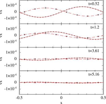
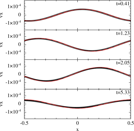
Figure 4: Time evolution of the gas (stars) and dust (open circles) components in the dustywave test with $\rho_{\rm D}/\rho_{\rm G}=1$ case. Dashed (dust) and solid (gas) lines represent the analytical solutions for the gas and dust components respectively. Left panels correspond to a low drag regime with $\delta t/t_{s}\approx 10^{-3}$ ($K_{\rm const}=1$), where 32 and 8 particles have been respectively used for the gas and dust components. The right panels correspond to a strong drag regime with $\delta t/t_{s}\approx 0.1$ ($K_{\rm const}=100$). A total of 128 dust and gas particles have been necessary in this case in order to reproduce the solution. In order to quantify the deviations of the numerical solutions with respect to the analytical solutions, the error norms can be calculated for both cases. At $t=5.33$, $L1=1.8\times 10^{-2}$, $L2=2\times 10^{-2}$, and $L3=3.4\times 10^{-2}$ for the $K_{\rm const}=1$ case, while $L1=1.2\times 10^{-1}$,$L2=1.3\times 10^{-1}$, and $L\infty=1.9\times 10^{-1}$ for the $K_{\rm const}=100$ case. In the latter case, a higher deviation from the analytical solution can be observed due to the presence of overdissipation.

The present method possesses two very different regimes, depending on the ratio between the gas integration time-scale $\delta t$, and the dust stopping time $t_{\rm s}$. If $\delta t/t_{s}\ll 1$ (when an explicit integration could be used)

$$\xi\approx\frac{K^{\rm E}_{\rm s}}{\hat{m}_{\rm D}}\rho_{\rm G}\delta t,$$ (62)

and equations 42, 43 and 44 thus become

$$\textbf{v}_{\rm D}^{i}( t+\delta t,\textbf{r}_{\rm i})\approx\textbf{v}_{\rm D}^{i}(t,\textbf{r}_{\rm i})$$ (63)

$$~{}~{}~{}~{}-\frac{\nu}{N_{\rm i}}\sum_{\rm k}^{\rm gas}m_{\rm k}\frac{K^{\rm E}_{\rm s}}{\hat{m}_{\rm D}}(\textbf{v}_{\rm ik}\cdot\hat{\textbf{r}}_{\rm ik})\hat{\textbf{r}}_{\rm ik}W(|\textbf{r}_{\rm ik}|,h_{\rm k})\delta t$$

$$=\textbf{v}_{\rm D}^{\rm i}(t,\textbf{r}_{\rm i})-\frac{K^{\rm E}_{\rm s}\rho_{\rm G}}{\hat{m}_{\rm D}}\textbf{v}_{\rm DG}(t,\textbf{r}_{\rm i})\delta t,$$

$$\textbf{v}_{\rm G}^{j}( t+\delta t,\textbf{r}_{\rm j})\approx\textbf{v}_{\rm G}^{j}(t,\textbf{r}_{\rm j})-\left.\frac{\nabla P_{\rm G}}{\rho_{\rm G}}\right|_{\textbf{r}_{\rm j}}\delta t$$ (64)

$$~{}~{}~{}~{}+\nu\sum_{\rm k}^{\rm dust}\frac{m_{\rm k}}{N_{\rm k}}\frac{K^{\rm E}_{\rm s,k}}{\hat{m}_{\rm D}}(\textbf{v}_{\rm kj}\cdot\hat{\textbf{r}}_{\rm kj})\hat{\textbf{r}}_{\rm kj}W(|\textbf{r}_{\rm jk}|,h_{\rm j})\delta t$$

$$=\textbf{v}_{\rm G}^{\rm j}(t,\textbf{r}_{\rm j})-\left.\frac{\nabla P_{\rm G}}{\rho_{\rm G}}\right|_{\textbf{r}_{\rm j}}\delta t+\frac{K^{\rm E}_{\rm s}\rho_{\rm D}}{\hat{m}_{\rm D}}\textbf{v}_{\rm DG}(t,\textbf{r}_{\rm j})\delta t,$$

$$u_{\rm G}^{j}( t+\delta t,\textbf{r}_{\rm j})\approx u_{\rm G}^{j}(t,\textbf{r}_{\rm j})-\left.\frac{P_{\rm G}(\nabla\cdot\textbf{v}_{\rm G})}{\rho_{\rm G}}\right|_{\textbf{r}_{\rm j}}\delta t$$ (65)

$$~{}~{}~{}~{}+\nu\sum_{\rm k}^{\rm dust}\frac{m_{\rm k}}{N_{\rm k}}\frac{K^{\rm E}_{\rm s,k}}{\hat{m}_{\rm D}}(\textbf{v}_{\rm kj}\cdot\hat{\textbf{r}}_{\rm kj})^{2}W(|\textbf{r}_{\rm jk}|,h_{\rm j})\delta t$$

$$=u_{\rm G}^{\rm j}(t,\textbf{r}_{\rm j})-\left.\frac{P_{\rm G}(\nabla\cdot\textbf{v}_{\rm G})}{\rho_{\rm G}}\right|_{\textbf{r}_{\rm j}}\delta t+\frac{K^{\rm E}_{\rm s}\rho_{\rm D}}{\hat{m}_{\rm D}}\textbf{v}^{2}_{\rm DG}(t,\textbf{r}_{\rm j})\delta t.$$

In this limit, the stability condition 61 becomes

$$\delta t<\frac{\hat{m}_{\rm D}}{K^{\rm E}_{\rm s}\rho_{\rm G}(1+\rho_{\rm D}/\rho_{\rm G})}=t_{\rm s},$$ (66)

coinciding with the Courant condition of an explicit integration as shown by Laibe & Price (2012a). Therefore, equations 63 to 65 will be equivalent to an explicit SPH two fluid method (Laibe & Price, 2012a) as long as very sharp density gradients are absent from the gas component. To quantify the errors produced by this approximation, the behaviour of the algorithm in the presence of strong density gradients (shocks) will be tested in section 3.3.

If, on the contrary, $\delta t/t_{\rm s}\gg 1$ (i.e. in the strong drag regime)

$$\xi\approx\frac{1}{1+\rho_{\rm D}/\rho_{\rm G}},$$ (67)

then equations 42, 43, and 44 become

$$\textbf{v}_{\rm D}^{i}(t +\delta t,\textbf{r}_{\rm i})=\nu\sum_{\rm k}^{\rm gas}\frac{m_{\rm k}}{\rho_{\rm k}}\left[\frac{\rho_{\rm i}\textbf{v}_{\rm i}+\rho_{\rm k}\textbf{v}_{\rm k}}{\rho_{\rm i}+\rho_{\rm k}}\cdot\hat{\textbf{r}}_{\rm ik}\right]\hat{\textbf{r}}_{\rm ik}W(|\textbf{r}_{\rm ik}|,h_{\rm k})$$ (68)

$$~{}~{}~{}~{}-\nu\sum_{\rm k}^{\rm gas}\frac{m_{\rm k}}{\rho_{\rm k}}\left(\frac{\nabla P_{\rm k}}{\rho_{\rm i}+\rho_{\rm k}}\cdot\hat{\textbf{r}}_{\rm ik}\right)\hat{\textbf{r}}_{\rm ik}W(|\textbf{r}_{\rm ik}|,h_{\rm k})\delta t$$

$$=\frac{\rho_{\rm D}\textbf{v}^{\rm i}_{\rm D}(t,\textbf{r}_{\rm i})+\rho_{\rm G}\textbf{v}_{\rm G}(t,\textbf{r}_{\rm i})}{\rho_{\rm D}+\rho_{\rm G}}-\left.\frac{\nabla P_{\rm G}}{\rho_{\rm D}+\rm\rho_{\rm G}}\right|_{\textbf{r}_{\rm i}}\delta t,$$

$$\textbf{v}_{\rm G}^{j}(t +\delta t,\textbf{r}_{\rm j})=\nu\sum_{\rm k}^{\rm dust}\frac{m_{\rm k}}{\rho_{\rm j}}\left[\frac{\rho_{\rm j}\textbf{v}_{\rm j}+\rho_{\rm k}\textbf{v}_{\rm k}}{\rho_{\rm j}+\rho_{\rm k}}\cdot\hat{\textbf{r}}_{\rm kj}\right]\hat{\textbf{r}}_{\rm kj}W(|\textbf{r}_{\rm kj}|,h_{\rm j})$$ (69)

$$~{}~{}~{}~{}-\nu\sum_{\rm k}^{\rm dust}\frac{m_{\rm k}}{\rho_{\rm k}}\left(\frac{\nabla P_{\rm j}}{\rho_{\rm k}+\rho_{\rm j}}\cdot\hat{\textbf{r}}_{\rm kj}\right)\hat{\textbf{r}}_{\rm kj}W(|\textbf{r}_{\rm kj}|,h_{\rm j})\delta t$$

$$=\frac{\rho_{\rm D}\textbf{v}_{\rm D}(t,\textbf{r}_{\rm j})+\rho_{\rm G}\textbf{v}^{\rm j}_{\rm G}(t,\textbf{r}_{\rm j})}{\rho_{\rm D}+\rho_{\rm G}}-\left.\frac{\nabla P_{\rm G}}{\rho_{\rm D}+\rm\rho_{\rm G}}\right|_{\textbf{r}_{\rm j}}\delta t,$$

$$u_{\rm G}^{j}(t+\delta t,\textbf{r}_{\rm j})=u_{\rm G}^{j}(t,\textbf{r}_{\rm j})-\left.\frac{P_{\rm G}(\nabla\cdot\textbf{v}_{\rm G})}{\rho_{\rm G}}\right|_{\textbf{r}_{\rm j}}\delta t$$ (70)

$$+\frac{\nu}{2}\sum_{\rm k}^{\rm dust}\frac{m_{\rm k}}{\rho_{\rm j}+\rho_{\rm k}}(\textbf{v}_{\rm kj}\cdot\hat{\textbf{r}}_{\rm kj}+\frac{\nabla P_{\rm j}}{\rho_{\rm j}}\cdot\hat{\textbf{r}}_{\rm kj}\delta t)^{2}W(|\textbf{r}_{\rm jk}|,h_{\rm j}),$$

which means that both components will be travelling, after the drag interaction, at the barycentric velocity of the fluid. Note that the last term of equation 70, just incorporate all the relative kinetic energy between the phases into thermal energy. In this regime, the algorithm removes all relative dust and gas motion by setting them in the barycentric velocity, and then applies an equal amount of pressure to both phases (equations 68 and 69). So, effectively, dust and gas phases behave as a single fluid with a modified sound speed (see for example Marble, 1970)

$$\hat{c}_{\rm s}=\frac{c_{\rm s}}{\sqrt{1+\rho_{\rm D}/\rho_{\rm G}}}.$$ (71)

It is interesting to note that in this limit, the evolution of the system is analogous to the one-fluid zeroth order approximation of Laibe & Price (2014a). In this limit, if the gas resolution is set too low, the first term in the right hand side of equations 68 and 69 will lead to an unphysical energy dissipation. One can easily visualize this phenomena by setting up a wave where gas particles are located in the wave antinodes and dust particles in the nodes. In this fiducial case, if equations 68 and 69 are applied, the resulting barycentric velocity will be zero, thus destroying all wave features. It is thus important to have a minimum gas resolution in order to guarantee a correct behaviour of the barycentric term. Additionally, for high dust-to-gas ratios, it will also be important to have equal gas and dust resolutions. If dust resolution is set too low, and dust and gas particles possess very different masses, the dust velocity will dominate in the barycentric term, and the one fluid limit will not be recovered. For low dust-to-gas ratios, overdissipative effects are reduced, since the fraction of momentum transferred between the phases (and thus the dissipated energy) will be diminished. Thus, it is possible to obtain the correct strong drag limit with an arbitrarily low number of dust particles. Overdissipation in the strong coupling limit, and the behaviour of the method as a function of the dust and gas resolutions will be tested in section 3.2.

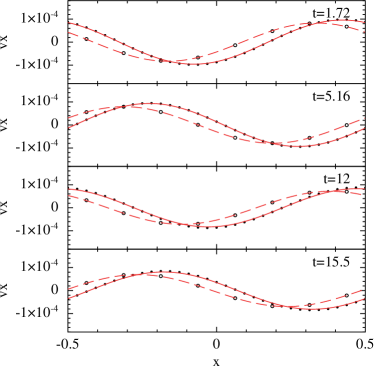
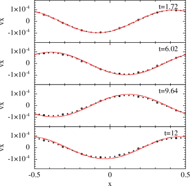
Figure 5: Time evolution of the gas (stars) and dust (open circles) components in the dustywave test with $\rho_{\rm D}/\rho_{\rm G}=0.01$. Dashed (dust) and solid (gas) lines represent the analytical solutions for the gas and dust components respectively. Left panels correspond to a low drag regime with $\delta t/t_{s}\approx 10^{-2}$ ($K_{\rm const}=0.1$), while right panels correspond to a high drag regime with $\delta t/t_{s}\approx 10$ ($K_{\rm const}=100$). A total of 32 gas particles and 8 dust particles have been used in both cases. Because of the relatively low fraction of momentum being transferred between the dust and gas phases, overdissipation has a negligible impact on the simulation, even if an arbitrarily small number of dust particles are used. The error norms for the $K_{\rm const}=0.1$ case at $t=15.5$ are $L1=2.9\times 10^{-2}$, $L2=3.2\times 10^{-2}$, and $L\infty=4.7\times 10^{-2}$, while the error norms for the $K_{\rm const}=100$ case at $t=12$ are $L1=7.3\times 10^{-2}$, $L2=8.4\times 10^{-2}$, and $L\infty=1.25\times 10^{-1}$.

It is also interesting to check whether the method can reproduce the properties of the dust and gas mixture in the so-called terminal velocity approximation (see for example Laibe & Price (2014a) and references therein). When dust and gas are strongly coupled, the dust reaches a constant relative velocity with respect to the gas, which is small but still finite. Such a relative velocity is proportional to the pressure gradient and the stopping time $t_{\rm s}$. One can see this by using

$$\mathcal{D}_{\rm t,G}\textbf{v}_{\rm G}(t,\textbf{r}_{\rm G})=\lim_{\delta t\rightarrow 0}\frac{{\bf v}_{\rm G}(t+\delta t,{\bf r}_{\rm G})-{\bf v}_{\rm G}(t,{\bf r}_{\rm G})}{\delta t}$$ (72)

$$=\lim_{\delta t\rightarrow 0}\sum_{\rm k}^{Dust}\frac{m_{\rm k}}{\delta t\rho_{\rm k}}\left[-(1-\xi)\frac{\nabla P_{\rm j}}{\rho_{\rm j}}\delta t+\xi(\textbf{v}_{\rm kj}\cdot\hat{\textbf{r}}_{\rm kj})\hat{\textbf{r}}_{\rm kj}\right]W(r_{\rm kj})$$

where we have introduced

$$\xi\equiv\frac{1-e^{-\delta t/t_{\rm s}}}{1+\rho_{\rm D}{\rho_{\rm G}}}$$ (73)

to simplify the notation. Now, in order to reach the terminal velocity, pressure gradient and drag forces must balance each other, leading to

$$0 =\sum_{\rm k}^{Dust}\frac{m_{\rm k}}{\delta t\rho_{\rm k}}\lim_{\delta t\rightarrow 0}\left[-(1-\xi)\frac{\nabla P_{\rm j}}{\rho_{\rm j}}\delta t+\xi(\textbf{v}_{\rm kj}\cdot\hat{\textbf{r}}_{\rm kj})\hat{\textbf{r}}_{\rm kj}\right]W(r_{\rm kj})$$ (74)

$$=\sum_{\rm k}^{Dust}\frac{m_{\rm k}}{\rho_{\rm k}}\left[-\frac{\nabla P_{\rm j}}{\rho_{\rm j}}+\frac{1}{t_{\rm s}}(\textbf{v}_{\rm kj}\cdot\hat{\textbf{r}}_{\rm kj})\hat{\textbf{r}}_{\rm kj}\right]W(r_{\rm kj})$$

which is simply the SPH equivalent of

$$\textbf{v}_{\rm DG}(t,\textbf{r}_{\rm G})=t_{\rm s}\frac{\nabla P_{\rm G}}{\rho_{\rm G}}$$ (75)

2.3 Dust evolution in the non-linear regime

The procedure followed in section 2.1 can be extended to the non-linear drag regimes as long as an approximate analytic solution can be found for the time evolution of the dust grains. For example, in a full non-linear regime (equations 8 and 11), a procedure analogous to the one in section 2.1 can be followed. In such a regime, the equations of motion of the dust and gas components can always be expressed as

$$\mathscr{D}_{\rm t,D}\textbf{v}_{\rm D}(t,\textbf{r}_{\rm D})=-\frac{K^{\rm St}_{\rm s}}{\hat{m}_{\rm D}}\rho_{\rm G}|\textbf{v}_{\rm DG}(t,\textbf{r}_{\rm D})|\textbf{v}_{\rm DG}(t,\textbf{r}_{\rm D}),$$ (76)

$$\mathcal{D}_{\rm D}\textbf{v}_{\rm G}(t,\textbf{r}_{\rm G})=\frac{K^{\rm St}_{\rm s}}{\hat{m}_{\rm D}}\rho_{\rm G}|\textbf{v}_{\rm DG}(t,\textbf{r}_{\rm G})|\textbf{v}_{\rm DG}(t,\textbf{r}_{\rm G}),$$ (77)

where $K_{\rm s}^{\rm St}\equiv\frac{1}{2}C_{\rm D}\pi s^{2}$. In this case, the chosen equations for a pair of arbitrary dust and gas fluid elements located at points $\textbf{r}_{\rm D}$ and $\textbf{r}_{\rm G}$ are

$$\textbf{v}_{\rm D}(t+\delta t,\textbf{r}_{\rm D}) =\textbf{v}_{\rm D}(t,\textbf{r}_{\rm D})$$ (78)

$$-\left(\frac{1-\frac{1}{1+\delta t/t_{\rm s}}}{1+\rho_{\rm D}/\rho_{\rm G}}\right)\textbf{v}_{\rm DG}(t,\textbf{r}_{\rm D}),$$

$$\textbf{v}_{\rm G}(t+\delta t,\textbf{r}_{\rm G}) =\textbf{v}_{\rm G}(t,\textbf{r}_{\rm G})$$ (79)

$$+\frac{\rho_{\rm D}}{\rho_{\rm G}}\left(\frac{1-\frac{1}{1+\delta t/t_{\rm s}}}{1+\rho_{\rm D}/\rho_{\rm G}}\right)\textbf{v}_{\rm DG}(t,\textbf{r}_{\rm G}),$$

$$u_{\rm G}(t+\delta t,\textbf{r}_{\rm G}) =u_{\rm G}(t,\textbf{r}_{\rm G})$$ (80)

$$+\frac{1}{2}\frac{\rho_{\rm D}}{\rho_{\rm G}}\left(\frac{1-\frac{1}{1+2\delta t/t_{\rm s}}}{1+\rho_{\rm D}/\rho_{\rm G}}\right)\textbf{v}^{2}_{\rm DG}(t,\textbf{r}_{\rm G}),$$

where

$$t_{\rm s}\equiv\frac{\hat{m}_{\rm D}}{K_{\rm s}^{\rm St}\rho_{\rm G}(1+\rho_{\rm D}/\rho_{\rm G})|\textbf{v}_{\rm DG}|}.$$ (81)

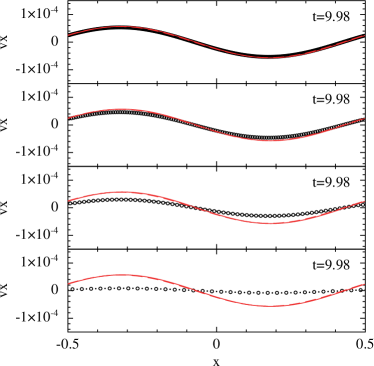
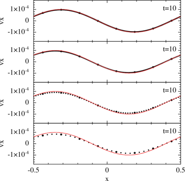
Figure 6: Comparison of the gas and dust velocities for several different resolutions in the dustywave test for a high drag regime ($K_{\rm const}=100$). From top to bottom a total of 256, 128, 64, and 32 particles have been used for the gas component. Left figure corresponds to a $\rho_{\rm D}/\rho_{\rm G}=1$ case with equal numbers of gas and dust particles, while right figure corresponds to a $\rho_{\rm D}/\rho_{\rm G}=0.01$, case with only 8 dust particles. In complete agreement with Laibe & Price (2012a,b) an excess of dissipation is found for low resolutions. However, for low dust-to-gas ratios, overdissipation effects becomes much less important even if a very low resolution is used.

By using SPH discretization, equations 78, 79 and 80 become

$$\textbf{v}^{\rm i}_{\rm D}(t+\delta t,\textbf{r}_{\rm i}) =\textbf{v}^{\rm i}_{\rm D}(t,\textbf{r}_{\rm i})$$ (82)

$$-\nu\sum_{\rm k}^{\rm gas}\frac{m_{\rm k}}{\rho_{\rm k}}\frac{1-\frac{1}{1+\delta t/t^{\rm i}_{\rm s}}}{1+\rho_{\rm i}/\rho_{\rm k}}(\textbf{v}_{\rm ik}\cdot\hat{\textbf{r}}_{\rm ik})\hat{\textbf{r}}_{\rm ik}W(|\textbf{r}_{\rm ik}|,h_{\rm k}),$$

$$\textbf{v}^{\rm j}_{\rm G}(t+\delta t,\textbf{r}_{\rm j}) =\textbf{v}^{\rm j}_{\rm G}(t,\textbf{r}_{\rm j})$$ (83)

$$+\nu\sum_{\rm k}^{\rm dust}\frac{m_{\rm k}}{\rho_{\rm j}}\frac{1-\frac{1}{1+\delta t/t^{\rm k}_{\rm s}}}{1+\rho_{\rm k}/\rho_{\rm j}}(\textbf{v}_{\rm kj}\cdot\hat{\textbf{r}}_{\rm kj})\hat{\textbf{r}}_{\rm kj}W(|\textbf{r}_{\rm kj}|,h_{\rm j}),$$

$$u^{\rm j}_{\rm G}(t+\delta t,\textbf{r}_{\rm j}) =u^{\rm j}_{\rm G}(t,\textbf{r}_{\rm j})$$ (84)

$$+\frac{\nu}{2}\sum_{\rm k}^{\rm dust}\frac{m_{\rm k}}{\rho_{\rm j}}\frac{1-\frac{1}{1+2\delta t/t^{\rm k}_{\rm s}}}{1+\rho_{\rm k}/\rho_{\rm j}}(\textbf{v}_{\rm kj}\cdot\hat{\textbf{r}}_{\rm kj})^{2}W(|\textbf{r}_{\rm kj}|,h_{\rm j}),$$

where in this case, an additional SPH summation is necessary to calculate $t^{\rm i}_{\rm s}$, since it depends on the relative velocity of the components at the dust particle location.

3 Numerical tests

To perform most of the numerical tests, the dragging algorithm was implemented in a purpose-built SPH code. The code included self-consistent $\rho$ and $h$ calculation, grad-h terms (Springel & Hernquist, 2002; Monaghan, 2002), and Riemann solver-like artificial viscosity with thermal conductivity whenever neeeded (Monaghan, 1997). To perform the Sedov test, the dragging algorithm was implemented into a well tested three-dimensional SPH code. For the sake of conciseness, the exact details of the SPH code will not be presented here, but the interested reader is referred to Ayliffe et. al (2012).

Figure 7: Results of the gas (stars) and dust (open circles) components of a shock-tube test with $\rho_{\rm G}/\rho_{\rm D}=1$ and 569 particles per phase. The left panels correspond to a constant drag regime with $K_{\rm s,const}/\hat{m}_{\rm D}=2$, whilst the right panels correspond to a non-linear regime (equations 8 and 11) with $K^{\rm St}_{\rm s}/\hat{m}_{\rm D}=2$. Dotted lines correspond to the long-term stationary solution of the problem, and have been added only as a guide. It has to be stressed out that no analytical solution exists for the transient case in this problem.

3.1 DUSTYBOX test in the Epstein regime

The dustybox test (Laibe & Price, 2011) was performed in order to prove the capacity of the method to reproduce the expected asymptotic behaviour of the drag force. A set of $20^{3}$ dust and $20^{3}$ gas particles with homogeneous densities $\rho_{\rm G}$ and $\rho_{\rm D}$ are placed in a periodic box with an initial velocity $\textbf{v}_{\rm D}=1$ and $\textbf{v}_{\rm G}=0$. In order to construct the initial model, particles are evenly distributed along a cubic lattice with $-0.5\leq x,y,z\leq 0.5$. The dust lattice is shifted, with respect to the gas, by half of the gas particles separation in each direction. The mass of each SPH particle is equal to

$$\centering m=\frac{V\rho}{N},\@add@centering$$ (85)

where $V$ is the computational domain volume, and $N$ the number of particles in each phase. An isothermal equation of state is adopted ($P=c_{\rm s}^{2}\rho_{\rm G}$), and in this case no artificial viscosity is used. The physical units of the problem are chosen such that $\rho_{\rm G}=10^{-9}$ g cm^-3, $\hat{\rho}_{\rm D}=3$  g cm^-3, $v_{\rm therm}=c_{\rm s}=10^{5}$ cm s^-1. These are the appropriate conditions for a dust particle at the mid-plane of a protoplanetary disk at 1 AU from the central star (see for example Armitage (2010)). The computational domain comprises a total volume of 1 cubic AU, and the total mass of gas inside the domain is $3.4\times 10^{30}$ g. The integration time-step $\delta t$ is calculated by finding the minimum value, for all gas particles, of

$$\delta t=\left(\frac{h}{c_{\rm s}}\right),$$ (86)

and

$$\delta t=0.1\left(\frac{h}{|\textbf{a}|}\right)^{1/2},$$ (87)

where $h$ is the SPH particle smoothing length and a is the gas particle acceleration. Since the pressure gradient is zero, the exact solution for equation (4) is easy to find in this case

$$\textbf{v}_{\rm DG}(t) =\textbf{v}_{\rm DG}(0)e^{-(t/t_{\rm s})},$$ (88)

allowing a direct comparison of the results obtained. In Fig. 1 the time evolution of the velocity of a single SPH dust particle is presented for several different values of the dust grain size $s$. Left figure corresponds to a case with $\rho_{\rm D}/\rho_{\rm G}=1$ while right figure corresponds to a case with $\rho_{\rm D}/\rho_{\rm G}=0.01$. As can be seen, irrespectively of the dust grain size, the correct terminal velocity between gas and dust components is reached in all cases. Whenever the gas integration time step becomes smaller than the dust stopping time, the algorithm is capable of following the velocity decay of the dust component towards its limiting velocity. If the dust stopping time becomes much smaller than the gas integration time step, the algorithm simply tries to put both components on their barycentric velocity, right from the start. If under any circumstance, resolving the velocity decay becomes essential, one can always artificially decrease the gas integration time-step by reducing the gas Courant time condition (equation 86) by an arbitrary factor. In Fig. 2 time evolution of the dust component velocity in the three-dimensional $\rho_{\rm D}/\rho_{\rm G}=0.01$, $s=1$ mm case is shown, for different values of the gas integration time step. As can be seen, since the stopping time is much shorter than the gas integration time-step ($t_{\rm s}\approx 4.5\times 10^{-5}$ yrs), an artificially reduced gas integration time-step is needed to start resolving the dust component velocity decay.

In order to better appreciate the precision of the adopted approximation, in Fig. 3, the relative errors in the $\rho_{\rm D}/\rho_{\rm G}=0.01$ test with $s=1$ m (left plot) and $s=1$ mm (right plot) are presented, for several different kernels. We test the standard $M_{4}$ cubic spline kernel (Monaghan, 1992), the $M_{6}$ quintic spline kernel, and the double hump cubic kernel (Fulk & Quinn, 1996; Laibe & Price, 2012a). As can be seen, the correct terminal velocity is obtained, irrespectively of the used kernel, with very high precision (the relative error between the numerical and analytical results is $\lesssim 10^{-4}\%$). The greatest departures from the analytical solution are obtained during the velocity decay phase. In this phase, only the double hump kernel keeps errors under acceptable limits. A similar result was also found by Laibe & Price (2012a) in their study. One can also see from the right plot of Fig. 3, that the normalization condition (equation 49), helps to reduce the errors further. If the double hump kernel is used in conjunction with the normalization condition, the maximum relative error is $\lesssim 1\%$ in all the tested cases. This is a very important results, since it shows that the trajectories of dust particles of arbitrary size can be accurately calculated, in a protoplanetary-like environment, without the need for excessive resolution.

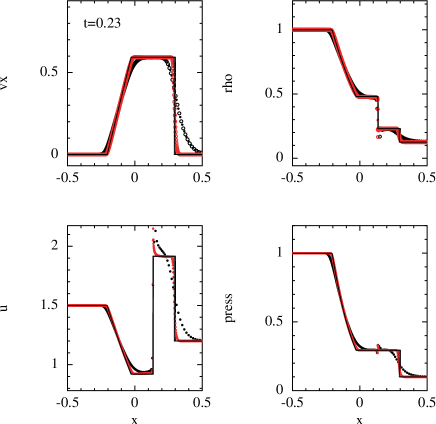
Figure 8: In the left plot, the $\rho_{\rm D}/\rho_{\rm G}=1$ shock-tube results in a high non-linear (equations 8 and 11) drag case with $K^{\rm St}_{\rm s}/\hat{m}_{\rm D}=100$ for two different resolutions; 256 particles per phase (red) and 2048 particles per phase (black). Results clearly converge towards the theoretical solution of the problem with the increase in particle resolution. Error norms for the velocity solution in the high resolution case are $L1=5.8\times 10^{-3}$, $L2=2.5\times 10^{-2}$ and $L\infty=5.1\times 10^{-1}$. In the right plot, a highly dragged case with $K^{\rm St}_{\rm s}/\hat{m}_{\rm D}=100$ with $\rho_{\rm D}/\rho_{\rm G}=0.01$ is presented for the non-linear regime. 569 gas and 50 dust particles have been used. As can be seen, despite the low number of dust particles used, no evidence of overdissipation is found.

3.2 DUSTYWAVE test

The second test performed was the study of the propagation of a sound wave in a dust-gas mixture in a constant drag regime, also known as the dustywave test (Laibe & Price, 2011). This can be done by setting the drag coefficients on a single grain, in the Epstein regime, to be equal to

$$K^{\rm E}_{\rm s}=\frac{K_{\rm s,const}}{\rho_{\rm G}}.$$ (89)

As a consequence, the equations of motion for the dust and gas components become

$$\mathcal{D}_{\rm t,D}\textbf{v}_{\rm D}(t,\textbf{r})=-\frac{K_{\rm s,const}}{\hat{m}_{\rm D}}\textbf{v}_{\rm DG}(t,\textbf{r})=-\frac{K_{\rm const}}{\rho_{\rm D}}\textbf{v}_{\rm DG}(t,\textbf{r}),$$ (90)

$$\mathcal{D}_{\rm t,G}\textbf{v}_{\rm G}(t,\textbf{r}) =\frac{K_{\rm s,const}}{\hat{m}_{\rm D}}\frac{\rho_{\rm D}}{\rho_{\rm G}}\textbf{v}_{\rm DG}(t,\textbf{r})$$ (91)

$$=-\frac{K_{\rm const}}{\rho_{\rm G}}\textbf{v}_{\rm DG}(t,\textbf{r}),$$

where we have introduced the drag coefficient per unit volume $K_{\rm const}\equiv K_{\rm s,const}\rho_{\rm D}/\hat{m}_{\rm D}$. This is a particularly interesting problem, because as in the previous case, it possesses an analytic solution (Laibe & Price, 2011). To set up the test, an ensemble of dust and gas particles with homogeneous densities $\rho_{\rm D}$ and $\rho_{\rm G}$ are evenly distributed over a periodic one-dimensional domain $-0.5\leq x\leq 0.5$. Particle masses are assigned in the same way as in the previous section. No artificial viscosity is used in this case in order to avoid introducing non-physical energy dissipation in the test. The integration time-step $\delta t$ is again calculated by finding the minimum value given by equations 86 and 87. An isothermal equation of state $P=c^{2}_{\rm s}\rho_{\rm G}$ with $c_{\rm s}=1$ is used in this case. In order to create the waves, a sinusoidal perturbation is introduced for each particle, both in position and velocity

$$x_{\rm p}=x-\delta_{x}\cos(2\pi x),$$ (92)

$$v_{\rm x,p}=-\delta_{v}\sin(2\pi x),$$ (93)

where $x$ is the original position of each particle, and $\delta_{v}=10^{-4}$, so that the velocity perturbation of the wave is $\delta v/c_{\rm s}=10^{-4}$. The spatial perturbation $\delta_{x}$ will be different for every resolution, and is selected in each case so that the density perturbation of the wave is always $\delta\rho/\rho=10^{-4}$. After introducing the perturbation, the propagation of the resulting sound wave within the domain is followed. As previously mentioned, we used the predictor-corrector integrator for this test, since it gives better long-term energy and momentum conservation.

Figure 9: Comparison of the $\rho_{\rm D}/\rho_{\rm G}=1$ shock tube test result with an explicit two-fluid approach (left plot) and our semi-implicit method (right plot) for a very high drag regime with $K_{\rm s,const}/\hat{m}_{\rm D}=10^{6}$. The resolution is the same in both cases; a total of 569 particles per phase. The semi-implicit method is capable of generating a much better solution, even without satisfying the resolution criteria $h<c_{\rm s}t_{\rm s}$. The explicit method requires many more integration time steps to reach the same moment in time, due to the Courant condition of the dust. Because of the error committed due to the lack of resolution at every step, a very high deviation from the analytical solution is found. The semi-implicit method, on the contrary, being only limited by the gas Courant condition, largely avoids this problem.

In Fig. 4, four different snapshots of the time evolution of the sound wave velocity in a $\rho_{\rm D}=1$, $\rho_{\rm G}=1$ case with $\delta t/t_{\rm s}\approx 10^{-3}$ ($K_{\rm const}=1$) (left panel), and $\delta t/t_{\rm s}\approx 10^{-1}$ ($K_{\rm const}=100$) (right panel), are presented. In Fig. 5, four different snapshots of the time evolution of the sound wave velocity in a $\rho_{\rm D}=0.01$, $\rho_{\rm G}=1$ case with $\delta t/t_{\rm s}\approx 10^{-2}$ ($K_{\rm const}=0.1$) (left panel), and $\delta t/t_{\rm s}\approx 10$ ($K_{\rm const}=100$) (right panel), are presented. As can be seen, a good agreement with the analytical solutions has been obtained in both cases. In order to quantify the deviation from the analytical solution several error norms are calculated (see figure captions)

$$L_{1}=\frac{1}{Nf_{\rm max}}\sum_{\rm i}^{N}(f_{\rm i}-f_{\rm exact}),$$ (94)

$$L_{2}=\left[\frac{1}{N}\left(f^{2}_{\rm max}\sum_{\rm i}^{N}(f_{\rm i}-f_{\rm exact})^{2}\right)\right]^{1/2},$$ (95)

$$L_{\infty}=\frac{1}{f_{\rm max}}{\rm max}_{\rm i}|f_{\rm i}-f_{\rm exact}|,$$ (96)

where $f_{\rm max}$ is the maximum value of the exact solution in the plotted region, $f_{\rm exact}$ is the analytical solution for the $i$-th point of the plot, and $N$ is the number of plotted points (http://users.monash.edu.au/dprice/$\sim$splash/userguide/). As previously mentioned, one of the most important characteristics of dust and gas mixtures is that the local sound speed modification as a function of the dust/gas fraction (equation 71). Since the analytical solutions seen in Fig. 4 and  5 take into account such a modification, the test confirms the capacity of the algorithm to reproduce this feature of dust/gas mixtures.

The results of Figs. 4 and  5 also confirm that, whenever the amount of momentum transferred between the phases is small compared with the total momentum of the gas, an arbitrarily low number of dust particles can be used. Both in the lower drag case of Fig. 4, and in Fig. 5 only 8 dust particles per wavelength are necessary to obtain reasonable results. Unfortunately, as can be seen in Fig. 6, a certain excess of energy dissipation by drag in the high drag regime becomes unavoidable. This is not a new phenomena and was already found by Laibe & Price (2012a, b) in their simulations. The SPH two fluid scheme needs a minimum resolution ($h<c_{\rm s}t_{\rm s}$) in order to correctly resolve the small position and velocity differences between the dust and gas phases, otherwise overdissipation becomes unavoidable. However, because our method treats only the gas as a fluid, and not the dust, this resolution criterion must only be satisfied by the gas component, not the dust. In Fig. 6, the effect of particle resolution is investigated in the high drag regime for two different dust-to-gas ratios. From top to bottom a total of 256, 128, 64 and 32 gas particles have been used. In the left panel of Fig. 6 a $\rho_{\rm D}/\rho_{\rm G}=1$ case with $K_{\rm const}=100$ is presented. In this case, equal numbers of gas and dust particles have been used. In the right panel of Fig. 6 a $\rho_{\rm D}/\rho_{\rm G}=0.01$ case with $K_{\rm const}=100$ is presented. In this case only 8 dust particles have been used. As can be seen, and in complete agreement with the minimum resolution condition, only the ones with a minimum number of $256$ gas and dust particles is capable of matching the expected solution in the $\rho_{\rm D}/\rho_{\rm G}=1$ case. However, in the $\rho_{\rm D}/\rho_{\rm G}=0.01$ case, overdissipation effects become much less dramatic, even with a very low gas and dust particle resolution. This is important, since most astrophysical applications have low dust-to-gas ratios. It is also important to note that the present method is less dissipative than the previous ones, because we need to perform many fewer integration time-steps, in order to evolve the simulation to a given time. In the present method, the interpolation error is only committed once per gas integration time step, in contrast with explicit or implicit methods where the error can be committed hundreds or thousands of times per gas integration time step. In fact, in earlier versions of the present method an iterative procedure was tried in order to achieve a higher precision in the final relative velocities between the components, but instead it resulted in a degree of overdissipation comparable to the one using a standard integration method.

3.3 Shocks in a dust-gas mixture

The next two tests are the shock tube test, and the Sedov blast test (Sedov, 1959). They were both performed in order to test the behaviour of the scheme, in the presence of strong density and pressure gradients. Since equation (16) will only be valid as long as no big changes in the density or the pressure gradient occur during the integration time-step, these experiments are critical to prove the usefulness of the method. In these experiments, thermal energy plays an essential role in the evolution of the system, so this time an adiabatic equation of state with $P=(\gamma-1)u\rho_{\rm G}$ and $\gamma=5/3$ is used. Also, to correctly model the shocks, Monaghan (1997) artificial viscosity is used in both cases with coefficients $\alpha=2$ and $\alpha_{\rm u}=1$ for the thermal conduction parameter. The signal velocities are $\textbf{v}_{\rm sig}=c_{\rm ij}-\textbf{v}_{\rm ij}\cdot\hat{\textbf{r}}_{\rm ij}$ and $\textbf{v}_{\rm sig,u}=|\textbf{v}_{\rm ij}\cdot\hat{\textbf{r}}_{\rm ij}|$ respectively. The time-step $\delta t$ is calculated in both cases by finding the minimum value for all gas particles between

$$\delta t=\frac{h}{|\textbf{v}_{\rm sig}|},$$ (97)

and

$$\delta t=0.1\left(\frac{h}{|\textbf{a}|}\right)^{0.5},$$ (98)

Figure 10: Particle density as a function of radius in the Sedov blast test in the $\rho_{\rm G}/\rho_{\rm D}=0.01$, and $\delta t/t_{s}\approx 1$ ($K_{\rm s,const}/\hat{m}_{\rm D}=100$) case. The dotted line corresponds to the self-similar solution of the gas-only Sedov problem and has been added as an approximate guide. Uppermost panels correspond to the solution obtained with the present algorithm and the lowermost panels correspond to the result obtained using an explicit integrator. Left plots correspond to the gas component, while right plots correspond to the dust component.

where a is the SPH gas particle acceleration. Note that if additional forces affecting both phases (like radiation pressure for example) were introduced in the simulation, condition 98 should also be taken into account for the dust particles. In these tests, the more restrictive conditions will occur at the shock front. To set up the shock tube test, an ensemble of particles with $\rho_{\rm L,G}=\rho_{\rm L,D}=1.0$, $\rho_{\rm R,G}=\rho_{\rm R,D}=0.125$, $P_{\rm L}=1.0$, $P_{\rm R}=0.1$, are evenly distributed in a one-dimensional bounded domain $-0.5\leq x\leq 0.5$. To model the density jump, a different number of particles is used at each side of the discontinuity. In particular, since it is a one-dimensional case

$$\frac{N_{\rm left}}{N_{\rm right}}=\left(\frac{\rho_{\rm left}}{\rho_{\rm right}}\right)N,$$ (99)

where $N$ is the total number of particles. Particle masses are calculated as in the previous sections.

Fig. 7, presents the results for two weakly dragged cases in a constant drag regime. The left panel represents a case with $K_{\rm s,const}/\hat{m}_{\rm D}=2$, while the right panel represents non linear drag regime (equations 8 and 11) with $K^{\rm St}_{\rm s}/\hat{m}_{\rm D}=2$. Despite not having an analytical solution for the transient phase, in both figures, the long-term analytical solution of the problem has been added (dotted line) as a guideline. In both cases, the obtained solution compares very favourably with the results previously obtained by Laibe & Price (2012a, b) through the use of explicit/implicit methods. In the left panel of Fig. 8, a strongly dragged case with $K_{\rm s}^{\rm St}/\hat{m}_{\rm D}=100$ is presented for two different resolutions in the non-linear regime. In this case, the analytical solution is known (solid line), and as can be seen, it is well matched by the numerical results if enough resolution is used. In the right panel of Fig. 8 the same case is presented for a $\rho_{\rm D}/\rho_{\rm G}=0.01$ case with 569 gas and 50 dust particles. As can be seen, despite the reduced dust resolution, the correct result is obtained and there is no evidence of overdissipation.

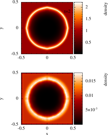
Figure 11: Cross sections of the mid-plane gas (top panel) and dust (lower panel) densities in the Sedov blast test for a extremely strong dragged case with $K_{\rm s,const}/\hat{m}_{\rm D}=10^{20}$. Such a calculation would be impossible with an explicit time step.

It is also very interesting to compare the results obtained using the semi-implicit method, with those obtained with an explicit integration scheme, for a very high drag regime with $K_{\rm s,const}/\hat{m}_{\rm D}=10^{6}$. As can be seen in Fig. 9, whereas excess dissipation in the explicit calculation gives an incorrect solution, our semi-implicit method avoids the problem. As previously mentioned, the source of overdissipation in the semi-implicit method comes from the incapacity of the algorithm to estimate the local barycentric velocity, due to the lack of resolution. However, and in contrast with an ordinary explicit method, if the semi-implicit method is used, the error in the barycentric velocity estimation is only committed once per gas integration time-step. On the contrary, if an explicit method is used, due to the Courant condition of the drag interaction, the error in the estimation of the drag acceleration is committed a lot more times per gas integration time-step, leading to a very poor result. This effect will also occur if a conventional implicit integration scheme is used (e.g. Laibe & Price, 2012b). Finally, in the uppermost panels of Fig. 10 the result of a Sedov blast test with $\rho_{\rm D}=0.01$, $\rho_{\rm G}=1$, and $\delta t/t_{s}\approx 1$ ($K_{\rm s,const}/\hat{m}_{\rm D}=100$) is presented. In this case, the gas integration time-step is set by the Courant time condition at the shock front. In the test, a total of $2\times 50^{3}$ particles are evenly distributed in a three-dimensional Cartesian grid with $-0.5\leq x,y,z\leq 0.5$. Particle masses are calculated as in the previous sections. The dust grid is displaced with respect to the gas one by half of the gas particle separation in each direction. To model the explosion a total thermal energy of $10^{-3}$ code units is distributed over the particles inside a certain radius ($r<2h$). As a comparison, the Sedov blast test performed with an ordinary explicit integration scheme, is also presented in the lower panels of Fig. 10. As can be seen, there are no significant differences.

Table 1: Computational time increase factors as a function of the drag strength in the Sedov test. The computational time of each simulation with the explicit method is divided by the computational time of the semi-implicit method. In the semi-implicit method, since the time-step of the simulation is exclusively determined by the gas Courant time condition, and the dust-to-gas ratio is small, no noticeable extra computational effort is needed if the drag strength is increased.

$K_{\rm s,const}/\hat{m}_{\rm D}$	Explicit/semi-implicit computational time
$10^{2}$	10
$10^{3}$	200
$10^{4}$	1500

Again, in this case, no evidence of the resolution limitation has been found, due to the lower density ratio between the gas and dust components. Since the typical gas-to-dust ratios in the interstellar medium are very similar to the ones used in the Sedov test, we expect the method to be useful in realistic astrophysical simulations. Additionally, we have used this test to compare the computational time of the method, with that of a traditional explicit integration. In table 1, a comparison of the computational time for several different drag strengths, is presented for both cases. In each case, the computational time spent by each simulation is divided by the computational time of the semi-implicit method in the $K_{\rm s,const}/\hat{m}_{\rm D}=100$ case. As can be seen, as the drag strength is increased, the explicit integrator computational time is increased, by several orders of magnitude, with respect to the computational time spent by semi-implicit method for $K_{\rm s,const}/\hat{m}_{\rm D}=100$. On the contrary, the computational time of the semi-implicit method remains stable, since the integration time-step is exclusively determined by the gas Courant condition, and is independent of the drag strength. As can be seen in Fig. 11, arbitrarily large values for the drag coefficient can be used. This value would be completely prohibitive in any two-fluid explicit integration method.

3.4 Dust settling in a gaseous disk in the Epstein regime.

The final test performed was the mid-plane settling of dust particles in a one-dimensional vertical section of an isothermal disk with $P=c^{2}_{\rm s}\rho_{\rm G}$ and $c_{\rm s}=1$. To set up the test, 100 gas and 100 dust particles, with $\rho_{\rm D}=0.01$ and $\rho_{\rm G}=1$, are evenly distributed over a one-dimensional domain ($-2<z<2$). Particle masses are assigned following the same procedure as in the previous sections. An external acceleration $a_{\rm ext,D}=a_{\rm ext,G}=-\Omega^{2}z$ is used to simulate the vertical component of the gravitational field from the star at the centre of the disk, where $\Omega$ is the angular frequency. (see Appendices A and B for a detailed explanation about how to implement external forces in the integration scheme). No boundaries have been used, and since one does not expect shocks to be important, the use of artificial viscosity is avoided. The evolution equations of the system are given by

$$\mathcal{D}_{\rm t,D}v_{\rm D}=-\frac{K^{\rm E}_{\rm s}}{\hat{m}_{\rm D}}\rho_{\rm G}\left(v_{\rm D}-v_{\rm G}\right)-\Omega^{2}z,$$ (100)

$$\mathcal{D}_{\rm t,G}v_{\rm G}=\frac{K_{\rm s}^{\rm E}}{\hat{m}_{\rm D}}\rho_{\rm D}\left(v_{\rm D}-v_{\rm G}\right)-\Omega^{2}z-\frac{1}{\rho_{\rm G}}\left(\frac{\partial P}{\partial z}\right).$$ (101)

In order for the system to relax, the gas particles are evolved under gravitational and pressure forces, until the hydrostatic equilibrium condition is attained. Whenever hydrostatic equilibrium is reached, equations 100 and 101 can be solved

$$0=-K_{\rm s}^{\rm E}\left(\frac{\rho_{\rm G}}{\hat{m}_{\rm D}}\right)\left(v_{\rm D}-v_{\rm G}\right)-\Omega^{2}z,$$ (102)

$$0=K_{\rm s}^{\rm E}\left(v_{\rm D}-v_{\rm G}\right)-\Omega^{2}z-\frac{c_{\rm s}^{2}}{\rho_{\rm G}}\left(\frac{\partial\rho_{\rm G}}{\partial z}\right),$$ (103)

giving the gas hydrostatic density profile:

$$\rho_{\rm G}(z) \approx\rho_{\rm G}(0)e^{-\Omega^{2}z^{2}/(2c^{2}_{\rm s})},$$ (104)

which is valid as long as $\rho_{\rm G}\gg\rho_{\rm D}$. In Fig. 12, the initial gas density profile of the isothermal disk is presented. As can be seen, the gas perfectly reproduces a Gaussian density profile with $\rho_{\rm G}(0)=1.622$, $c_{\rm s}=0.98$ and $\Omega=1$. After gas relaxation, drag forces are switched on, and evolution is started again. If the drag coefficient $K_{\rm s}^{\rm E}/\hat{m}_{\rm D}$ is high enough, dust particles reach a limiting velocity, given by the solution of equations 102 and 103.

$$v_{\rm D}(z)-v_{\rm G}(z)=-\left(\frac{\Omega^{2}\hat{m}_{\rm D}}{K_{\rm s}^{\rm E}\rho_{\rm G}(0)}\right)ze^{\Omega^{2}z^{2}/(2c_{\rm s}^{2})}.$$ (105)

In Fig. 13, the dust component velocity as a function of $z$ is presented for two cases ($K_{\rm s}^{\rm E}/\hat{m}_{\rm D}=10$ and $K_{\rm s}^{\rm E}/\hat{m}_{\rm D}=100$). As can be seen, the correct limiting velocity of the dust component is reached in both cases. Because $\rho_{\rm D}/\rho_{G}=0.01$, the momentum transferred between the dust and gas phases is rather small, and the gas component remains very close to the hydrostatic equilibrium. As can be seen in the $K_{\rm s}^{\rm E}/\hat{m}_{\rm D}=100$ case (right plot), dust particles almost instantaneously reach its limiting velocity. On the contrary, if $K_{\rm s}^{\rm E}/\hat{m}_{\rm D}=10$ (left plot), particles need more time to reach the limiting velocity and the transitory state can be seen for $\mid z\mid>1.2$. In order to check whether the algorithm is capable of correctly reproducing such a transitory regime, the velocity as a function of $z$ for a single SPH dust particle can be compared with the numerical solution of equations 100 and 101. In Fig. 14 the evolution of a single SPH dust particle is plotted for three different $K_{\rm s}^{\rm E}$ values. Circles represent the velocity of the particle, for different time steps, as it falls down towards the disk mid-plane. Dashed lines represent the numerical solution of equations 100 and 101 for each case, while solid lines represent the limiting velocity for each case as given by equation 105. If $K_{\rm s}^{\rm E}/\hat{m}_{\rm D}=0.01$, the particle does not have time to reach the limiting velocity, and simply suffers velocity damping while it oscillates around the disk mid-plane. As can be seen, a perfect agreement is achieved with the theoretical behaviour. If $K_{\rm s}^{\rm E}/\hat{m}_{\rm D}=10$, the dust particle reaches the limiting velocity at $z\simeq-1.2$, in perfect agreement with the numerical solution of equations 100 and 101, and explaining the global velocity profile of the dust component (as seen in Fig. 13). For $K_{\rm s}^{\rm E}/\hat{m}_{\rm D}=100$, although the theoretical solution is approximately obtained, some oscillations of the particle velocity can be observed. Such oscillations occur due to the low number of gas particles present in the outermost parts of the disk. If a higher resolution simulation is performed (1000 gas particles), the oscillations disappear, and the velocity of the dust particle closely matches the analytical solution.

Figure 12: Initial gas density profile of the relaxed disk as a function of z. A total of 100 gas particles have been used to model the vertical disk profile. Dots correspond to the gas particles whereas the dashed line corresponds to a Gaussian profile, as predicted by equation 104.

Figure 13: Velocity of the dust component as a function of $z$ in the dust settling test. Dots correspond to the gas particles, while open circles correspond to the dust particles. The left plot corresponds to a $K^{\rm E}_{\rm s}=0.1$ case, whereas the right plot corresponds to a $K^{\rm E}_{\rm s}=1.0$ case. The dashed line corresponds to the stationary solution of the problem in each case, as shown in equation 105. In the $K^{\rm E}_{\rm s}=0.1$ case, due to the weakness of the drag force, the outermost dust particles ($|z|>1.2$) are still in the transient state.

Figure 14: Velocity of a single dust particle as a function of $z$ for different $K^{\rm E}_{\rm s}$ values in the dust settling test. Circles correspond to the particle velocity at different time steps. Dashed lines correspond to the numerical solution of equations 100 and 101, while solid lines represent the limiting velocity for each case as given by equation 105. As can be seen, the higher $K^{\rm E}_{\rm s}$ is, the sooner the limiting velocity is reached, as expected. In the $K^{\rm E}_{\rm s}=1$ case, some oscillations of the dust particle velocity are found in the outermost part of the disk, due to the low number of gas particles. If a second simulation with 1000 gas and 1000 dust particles is performed (low right plot), the trajectory of the dust particle becomes free from oscillations, and closely matches the analytical solution.

4 Conclusions

A new method has been proposed to avoid explicit integration of the time evolution equations of small dust grains in the two fluid SPH approach. Through the use of semi-analytic solutions for the decay of the gas and dust relative velocity, the present method has been able to reproduce all the features of the previous two fluid SPH approach of Laibe & Price (2012a, b), with the advantage of a considerable gain in computational time in strong drag regimes. Due to its strictly dissipative nature, the velocity changes induced by the drag force can be estimated without the need for explicit acceleration recalculations or iterative procedures, even when the stopping time becomes much shorter than the gas evolutionary time-scale. The method is numerically stable, and always provides convergence towards the analytical solutions as the resolution is increased.

The method has also been capable of reproducing the correct behaviour of the drag force for all regimes. In the weak drag regime, the method is theoretically equivalent to a standard explicit integration, both in accuracy and computational efficiency, as long as strong gradients are not present in the immediate neighbourhood of dust particles. In the high drag regime, the method is capable of reproducing all the expected features of dust/gas mixtures. The results obtained in the test cases are completely analogous to those found by Laibe & Price (2012a, b) through the use of standard explicit and implicit methods.

In agreement with previous studies (Laibe & Price, 2012a, b), a resolution limit has been found for the method in the dustywave experiment. For high drag regimes with dust-to-gas ratios of order unity, the resolution should exceed $h<c_{\rm s}t_{\rm s}$ in order to avoid overdissipation. However, in the shock tube experiment, our method avoids the effects of overdissipation, which until now has been considered to be one of the main limitations of the two-fluid SPH approach. Furthermore, it has also been demonstrated that for low drag regimes, and even for high drag regimes with low dust-to-gas ratios, the number of dust particles present in the simulation becomes irrelevant, and the accuracy of the solution is only dependent on having sufficient gas resolution. Since in the vast majority of astrophysical applications the dust-to-gas ratio is expected to be rather low, only a good gas resolution will be necessary to avoid overdissipation. However, special attention must be payed to this limitation, since it will be very difficult to completely avoid overdissipation in complex global simulations, especially if one expects abrupt changes in the dust-to-gas ratios.

Appendix A Runge-Kutta-Fehlberg integrator

In order to capture both the gas and dust evolution described by equations 1, 2, 3, 4, and 5, the dust-gas drag equations must be coupled with an explicit hydrodynamical integrator. Combination with an integrator incorporating the gas pressure gradients is needed. One chosen integrator is a second order Runge-Kutta-Fehlberg scheme and the combined scheme can be summarized as follows

$$\tilde{\textbf{v}}^{t+1/2}_{\rm D} =\textbf{v}^{t}_{\rm D}+\textbf{a}_{\rm ext,D}^{\rm t}\delta t/2,$$ (106)

$$\tilde{\textbf{v}}^{t+1/2}_{\rm G} =\textbf{v}^{t}_{\rm G}-\left(\frac{\mathbf{\nabla}P}{\rho_{\rm G}}\right)_{t}\delta t/2+\textbf{a}_{\rm ext,G}^{\rm t}\delta t/2,$$

$$\textbf{v}^{t+1/2}_{\rm D} =\tilde{\textbf{v}}^{t+1/2}_{\rm D}-\xi(\tilde{\textbf{v}}^{t+1/2}_{\rm D}-\tilde{\textbf{v}}^{t+1/2}_{\rm G}),$$

$$\textbf{v}^{t+1/2}_{\rm G} =\tilde{\textbf{v}}^{t+1/2}_{\rm G}+\frac{\rho_{\rm D}}{\rho_{\rm G}}\xi(\tilde{\textbf{v}}^{t+1/2}_{\rm D}-\tilde{\textbf{v}}^{t+1/2}_{\rm G}),$$

$$\textbf{r}^{t+1/2}_{\rm D} =\textbf{r}^{t}_{\rm D}+\textbf{v}^{t}_{\rm D}\delta t/2,$$

$$\textbf{r}^{t+1/2}_{\rm G} =\textbf{r}^{t}_{\rm G}+\textbf{v}^{t}_{\rm G}\delta t/2,$$

for the first half of the time-step, and

$$\tilde{\textbf{v}}^{t+1}_{\rm D} =\textbf{v}^{t}_{\rm D}+\frac{1}{256}\textbf{a}_{\rm ext,D}^{\rm t}\delta t+\frac{255}{256}\textbf{a}_{\rm ext,D}^{t+1/2}\delta t,$$ (107)

$$\tilde{\textbf{v}}^{t+1}_{\rm G} =\textbf{v}^{t}_{\rm G}-\frac{1}{256}\left(\frac{\mathbf{\nabla}P}{\rho_{\rm G}}\right)_{t}\delta t-\frac{255}{256}\left(\frac{\mathbf{\nabla}P}{\rho_{\rm G}}\right)_{t+1/2}\delta t$$

$$+\frac{1}{256}\textbf{a}_{\rm ext,G}^{\rm t}\delta t+\frac{255}{256}\textbf{a}_{\rm ext,G}^{t+1/2}\delta t,$$

$$\textbf{v}^{t+1}_{\rm D} =\tilde{\textbf{v}}^{t+1}_{\rm D}-\xi(\tilde{\textbf{v}}^{t+1}_{\rm D}-\tilde{\textbf{v}}^{t+1}_{\rm G}),$$

$$\textbf{v}^{t+1}_{\rm G} =\tilde{\textbf{v}}^{t+1}_{\rm G}+\frac{\rho_{\rm D}}{\rho_{\rm G}}\xi(\tilde{\textbf{v}}^{t+1}_{\rm D}-\tilde{\textbf{v}}^{t+1}_{\rm G}),$$

$$\textbf{r}^{t+1}_{\rm D} =\textbf{r}^{t}_{\rm D}+\frac{1}{256}\textbf{v}^{t}_{\rm D}\delta t+\frac{255}{256}\textbf{v}^{t+1}_{\rm D}\delta t,$$

$$\textbf{r}^{t+1}_{\rm G} =\textbf{r}^{t}_{\rm G}+\frac{1}{256}\textbf{v}^{t}_{\rm G}\delta t+\frac{255}{256}\textbf{v}^{t+1}_{\rm G}\delta t,$$

for the full time-step. We have introduced the dust and gas components external accelerations $\textbf{a}_{\rm ext,D}$ and $\textbf{a}_{\rm ext,G}$, in order to account for forces like gravity, physical viscosity or radiation pressure. This method relies on the possibility of considering pressure and drag forces as separable interactions. As the performed tests have shown, it seems to be a good assumption.

Another particularly useful property of the present method is its capacity to predict the correct modified sound speed of the dust/gas mixture, as a function of the dust/gas ratio. By substituting the pre-dragged quantities $\tilde{\textbf{v}}^{\rm G}$ and $\tilde{\textbf{v}}^{\rm D}$ and the expression for the $\xi$ parameter into the $\textbf{v}^{\rm G}$ and $\textbf{v}^{\rm D}$ equations, one can convert the two-step method into an equivalent one-step method given by the set of equations for the first half of the time-step

$$\textbf{v}^{t+1/2}_{\rm D} =\textbf{v}^{t}_{\rm D}+\textbf{a}^{\rm t}_{\rm ext,D}\delta t/2-\frac{\rho_{\rm G}}{\rho^{*}}\left(\textbf{v}^{t}_{\rm DG}+\textbf{a}^{t}_{\rm ext,DG}\delta t/2\right)$$ (108)

$$-\left(\frac{\mathbf{\nabla}P}{\rho^{*}}\right)_{t}\delta t/2,$$

$$\textbf{v}^{t+1/2}_{\rm G} =\textbf{v}^{t}_{\rm G}+\textbf{a}^{\rm t}_{\rm ext,G}\delta t/2+\frac{\rho_{\rm D}}{\rho^{*}}\left(\textbf{v}^{t}_{\rm DG}+\textbf{a}^{t}_{\rm ext,DG}\delta t/2\right)$$

$$-\left(\frac{\mathbf{\nabla}P}{\rho^{**}}\right)_{t}\delta t/2,$$

$$\textbf{r}^{t+1/2}_{\rm D} =\textbf{r}^{t}_{\rm D}+\textbf{v}^{t}_{\rm D}\delta t/2,$$

$$\textbf{r}^{t+1/2}_{\rm G} =\textbf{r}^{t}_{\rm G}+\textbf{v}^{t}_{\rm G}\delta t/2,$$

where $\textbf{v}^{t}_{\rm DG}\equiv\textbf{v}^{t}_{\rm D}-\textbf{v}^{t}_{\rm G}$, $\textbf{a}^{t}_{\rm DG}\equiv\textbf{a}^{t}_{\rm D}-\textbf{a}^{t}_{\rm G}$ and

$$\textbf{v}^{t+1}_{\rm D} =\textbf{v}^{t}_{\rm D}+\frac{1}{256}\textbf{a}^{\rm t}_{\rm ext,D}\delta t+\frac{255}{256}\textbf{a}^{\rm t+1/2}_{\rm ext,D}\delta t$$ (109)

$$-\frac{1}{256}\left(\frac{\mathbf{\nabla}P}{\rho^{*}}\right)_{t}\delta t-\frac{255}{256}\left(\frac{\mathbf{\nabla}P}{\rho^{*}}\right)_{t+1/2}\delta t$$

$$-\frac{\rho_{\rm G}}{\rho^{*}}\left(\textbf{v}^{t}_{\rm DG}+\frac{1}{256}\textbf{a}^{\rm t}_{\rm ext,DG}\delta t+\frac{255}{256}\textbf{a}^{\rm t+1/2}_{\rm ext,DG}\delta t\right),$$

$$\textbf{v}^{t+1}_{\rm G} =\textbf{v}^{t}_{\rm G}+\frac{1}{256}\textbf{a}^{\rm t}_{\rm ext,G}\delta t+\frac{255}{256}\textbf{a}^{\rm t+1/2}_{\rm ext,G}\delta t$$

$$-\frac{1}{256}\left(\frac{\mathbf{\nabla}P}{\rho^{**}}\right)_{t}\delta t-\frac{255}{256}\left(\frac{\mathbf{\nabla}P}{\rho^{**}}\right)_{t+1/2}\delta t$$

$$+\frac{\rho_{\rm D}}{\rho^{*}}\left(\textbf{v}^{t}_{\rm DG}+\frac{1}{256}\textbf{a}^{\rm t}_{\rm ext,DG}\delta t+\frac{255}{256}\textbf{a}^{\rm t+1/2}_{\rm ext,DG}\delta t\right),$$

for the full time-step, where we have defined

$$\rho^{*} \equiv\frac{\rho_{\rm D}+\rho_{\rm G}}{1-e^{-\delta t/t_{\rm s}}},$$ (110)

$$\rho^{**} \equiv\frac{\rho_{\rm D}+\rho_{\rm G}}{1+\left(\frac{\rho_{\rm D}}{\rho_{\rm G}}\right)e^{-\delta t/t_{\rm s}}}.$$

As we can see, in this set of equations, dust can be no longer considered pressureless. It suffers an acceleration due to pressure gradient, and possesses an effective density $\rho^{*}$. This result can be understood if one realizes that a purely dissipative force does not always lead to a velocity decrease. Because drag is a purely dissipative force, it will always lead to a decrease in the relative velocity between dust and gas components. But sometimes, the only way to decrease such a relative velocity is to accelerate the dust component. Also, the effective densities $\rho^{*}$ and $\rho^{**}$ can be understood as the effective inertial response of the dust and gas components to the effective pressure terms. The weaker the drag force is, the higher the pressure gradient must be to accelerate the dust component. If $\delta t/t_{\rm s}\ll 1$, $\rho^{*}\rightarrow\infty$, $\rho^{**}\rightarrow\rho_{\rm G}$, and the equations for the change in velocity of the dust and gas components become

$$\textbf{v}^{t+1/2}_{\rm D} =\textbf{v}^{t}_{\rm D}+\textbf{a}^{\rm t}_{\rm ext,D}\delta t/2,$$ (111)

$$\textbf{v}^{t+1/2}_{\rm G} =\textbf{v}^{t}_{\rm G}-\left(\frac{\mathbf{\nabla}P}{\rho_{\rm G}}\right)_{t}\delta t/2+\textbf{a}^{\rm t}_{\rm ext,G}\delta t/2,$$

for the first half time-step and

$$\textbf{v}^{t+1}_{\rm D} =\textbf{v}^{t+1/2}_{\rm D}+\frac{1}{256}\textbf{a}^{\rm t}_{\rm ext,D}\delta t+\frac{255}{256}\textbf{a}^{\rm t+1/2}_{\rm ext,D}\delta t,$$ (112)

$$\textbf{v}^{t+1}_{\rm G} =\textbf{v}^{t+1/2}_{\rm G}-\frac{1}{256}\left(\frac{\mathbf{\nabla}P}{\rho_{\rm G}}\right)_{t}\delta t-\frac{255}{256}\left(\frac{\mathbf{\nabla}P}{\rho_{\rm G}}\right)_{t+1/2}\delta t$$

$$+\frac{1}{256}\textbf{a}^{\rm t}_{\rm ext,G}\delta t+\frac{255}{256}\textbf{a}^{\rm t+1/2}_{\rm ext,G}\delta t,$$

for the full time-step. The effective dust density term $\rho^{*}$ has become infinitely big, so the dust does not respond at all to the pressure gradient terms. That is, gas and dust decouple, and gas evolves as a single component fluid with sound speed $c_{\rm s}$. If, on the contrary, $\delta t/t_{\rm s}\gg 1$, $\rho^{*}\rightarrow\rho_{\rm D}+\rho_{\rm G}$, $\rho^{**}\rightarrow\rho_{\rm D}+\rho_{\rm G}$, and the equations for the change in velocity of the dust and gas components become this time

$$\textbf{v}^{t+1/2}_{\rm D} =\frac{\rho_{\rm D}\textbf{v}_{\rm D}^{t}+\rho_{\rm G}\textbf{v}_{G}^{t}}{\rho_{\rm D}+\rho_{\rm G}}-\left(\frac{\mathbf{\nabla}P}{\rho_{\rm D}+\rho_{\rm G}}\right)_{t}\delta t/2$$ (113)

$$+\frac{\rho_{\rm D}\textbf{a}_{\rm ext,D}^{t}+\rho_{\rm G}\textbf{a}_{\rm ext,G}^{t}}{\rho_{\rm D}+\rho_{\rm G}}\delta t/2,$$

$$\textbf{v}^{t+1/2}_{\rm G} =\frac{\rho_{\rm D}\textbf{v}_{\rm D}^{t}+\rho_{\rm G}\textbf{v}_{G}^{t}}{\rho_{\rm D}+\rho_{\rm G}}-\left(\frac{\mathbf{\nabla}P}{\rho_{\rm D}+\rho_{\rm G}}\right)_{t}\delta t/2$$

$$+\frac{\rho_{\rm D}\textbf{a}_{\rm ext,D}^{t}+\rho_{\rm G}\textbf{a}_{\rm ext,G}^{t}}{\rho_{\rm D}+\rho_{\rm G}}\delta t/2,$$

for the first half time-step and

$$\textbf{v}^{t+1}_{\rm D} =\frac{\rho_{\rm D}\textbf{v}_{\rm D}^{t}+\rho_{\rm G}\textbf{v}_{G}^{t}}{\rho_{\rm D}+\rho_{\rm G}}-\left(\frac{1}{256}\right)\left(\frac{\mathbf{\nabla}P}{\rho_{\rm D}+\rho_{\rm G}}\right)_{t}\delta t$$ (114)

$$-\frac{255}{256}\left(\frac{\mathbf{\nabla}P}{\rho_{\rm D}+\rho_{\rm G}}\right)_{t+1/2}\delta t$$

$$+\frac{1}{255}\frac{\rho_{\rm D}\textbf{a}_{\rm ext,D}^{t}+\rho_{\rm G}\textbf{a}_{\rm ext,G}^{t}}{\rho_{\rm D}+\rho_{\rm G}}\delta t$$

$$+\frac{255}{256}\frac{\rho_{\rm D}\textbf{a}_{\rm ext,D}^{t+1/2}+\rho_{\rm G}\textbf{a}_{\rm ext,G}^{t+1/2}}{\rho_{\rm D}+\rho_{\rm G}}\delta t,$$

$$\textbf{v}^{t+1}_{\rm G} =\frac{\rho_{\rm D}\textbf{v}_{\rm D}^{t}+\rho_{\rm G}\textbf{v}_{G}^{t}}{\rho_{\rm D}+\rho_{\rm G}}-\frac{1}{256}\left(\frac{\mathbf{\nabla}P}{\rho_{\rm D}+\rho_{\rm G}}\right)_{t}\delta t-$$

$$-\frac{255}{256}\left(\frac{\mathbf{\nabla}P}{\rho_{\rm D}+\rho_{\rm G}}\right)_{t+1/2}\delta t$$

$$+\frac{1}{255}\frac{\rho_{\rm D}\textbf{a}_{\rm ext,D}^{t}+\rho_{\rm G}\textbf{a}_{\rm ext,G}^{t}}{\rho_{\rm D}+\rho_{\rm G}}\delta t$$

$$+\frac{255}{256}\frac{\rho_{\rm D}\textbf{a}_{\rm ext,D}^{t+1/2}+\rho_{\rm G}\textbf{a}_{\rm ext,G}^{t+1/2}}{\rho_{\rm D}+\rho_{\rm G}}\delta t,$$

for the full time-step. Both effective density terms $\rho^{*}$ and $\rho^{**}$ become equal, so both dust and gas components evolve as a single component fluid, with the total mass of the mixture being advected. However, and since only the gas component can produce real pressure, they travel with a modified sound speed $\hat{c}_{\rm s}=c_{\rm s}/\sqrt{1+\rho_{\rm D}/\rho_{\rm G}}$, exactly as predicted by theory (see for example Marble (1970)). As can be seen in equations A9, both phases adopt in this regime the barycentric velocity in just one time-step, as it corresponds to a case where $\delta t/t_{\rm s}\gg 0$.

Despite being particularly useful to visualize the behaviour of dust and gas mixtures, and to show that the effective sound speed of the mixture is the expected one in the strong drag regime, we still recommend using the two-step method given by equations A1 and A2. It is clearly technically easier to implement into a pre-existing SPH code.

Appendix B Predictor-corrector integrator

The second chosen integrator was a modification of the predictor-corrector scheme of Serna et al. (1995) and it can be summarized as follows

$$\tilde{\textbf{v}}^{t+1/2}_{\rm D} =\textbf{v}^{t}_{\rm D}+\textbf{a}^{\rm t}_{\rm ext,D}\delta t,$$ (115)

$$\tilde{\textbf{v}}^{t+1/2}_{\rm G} =\textbf{v}^{t}_{\rm G}-\left(\frac{\mathbf{\nabla}P}{\rho_{\rm G}}\right)_{t}\delta t+\textbf{a}^{\rm t}_{\rm ext,G}\delta t,$$

$$\textbf{v}^{t+1/2}_{\rm D} =\tilde{\textbf{v}}^{t+1/2}_{\rm D}-\xi(\tilde{\textbf{v}}^{t+1/2}_{\rm D}-\tilde{\textbf{v}}^{t+1/2}_{\rm G}),$$

$$\textbf{v}^{t+1/2}_{\rm G} =\tilde{\textbf{v}}^{t+1/2}_{\rm G}+\frac{\rho_{\rm D}}{\rho_{\rm G}}\xi(\tilde{\textbf{v}}^{t+1/2}_{\rm D}-\tilde{\textbf{v}}^{t+1/2}_{\rm G}),$$

$$\textbf{r}^{t+1/2}_{\rm D} =\textbf{r}^{t}_{\rm D}+(\textbf{v}^{t+1/2}_{\rm D}+\textbf{v}^{t}_{\rm D})\delta t/2,$$

$$\textbf{r}^{t+1/2}_{\rm G} =\textbf{r}^{t}_{\rm G}+(\textbf{v}^{t+1/2}_{\rm G}+\textbf{v}^{t}_{\rm G})\delta t/2,$$

for the predictor phase and

$$\tilde{\textbf{v}}^{t+1}_{\rm D} =\textbf{v}^{t+1/2}_{\rm D}+\left[\textbf{a}_{\rm ext,D}^{t+1/2}-\textbf{a}_{\rm ext,D}^{t}\right]\delta t/2,$$ (116)

$$\tilde{\textbf{v}}^{t+1}_{\rm G} =\textbf{v}^{t+1/2}_{\rm G}-\left[\left(\frac{\mathbf{\nabla}P}{\rho_{\rm G}}\right)_{t+1/2}-\left(\frac{\mathbf{\nabla}P}{\rho_{\rm G}}\right)_{t}\right]\delta t/2+\left[\textbf{a}_{\rm ext,G}^{t+1/2}-\textbf{a}_{\rm ext,G}^{t}\right]\delta t/2,$$

$$\textbf{v}^{t+1}_{\rm D} =\tilde{\textbf{v}}^{t+1}_{\rm D}-\xi\left[(\tilde{\textbf{v}}^{t+1}_{\rm D}-\tilde{\textbf{v}}^{t+1}_{\rm G})-(\textbf{v}^{t+1/2}_{\rm D}-\textbf{v}^{t+1/2}_{\rm G})\right],$$

$$\textbf{v}^{t+1}_{\rm G} =\tilde{\textbf{v}}^{t+1}_{\rm G}+\frac{\rho_{\rm D}}{\rho_{\rm G}}\xi\left[(\tilde{\textbf{v}}^{t+1}_{\rm D}-\tilde{\textbf{v}}^{t+1}_{\rm G})-(\textbf{v}^{t+1/2}_{\rm D}-\textbf{v}^{t+1/2}_{\rm G})\right],$$

$$\textbf{r}^{t+1}_{\rm D} =\textbf{r}^{t+1/2}_{\rm D}+(\textbf{v}^{t+1}_{\rm D}-\textbf{v}^{t+1/2}_{\rm D})\delta t/3,$$

$$\textbf{r}^{t+1}_{\rm G} =\textbf{r}^{t+1/2}_{\rm G}+(\textbf{v}^{t+1}_{\rm G}-\textbf{v}^{t+1/2}_{\rm G})\delta t/3,$$

for the corrector phase.

References

Armitage (2010) Armitage P. J.,2010,
Cambridge University Press
Ayliffe et. al (2012) Ayliffe B. A.,
Laibe G., Price D. J., Bate M. R, 2011, MNRAS, 423, 1450
Bate (1995) Bate M., 1995, PhD thesis,
Univ. Cambridge
Fehlberg (1968) Fehlberg E., Low-order
classical Runge-Kutta formulas with step size control and their application to
some heat transfer problems, NASA Technical Report 315
Whipple (1972) Whipple, F.L., 1972, From
plasma to planet, ed A. Elvius, Wiley, London, p.211
Wetzstein (2009) Wtezstein M., Nelson A. F.,
Naab T., Burkert A., 2009, ApJS, 184, 298