Gyratonic pp-waves and their impulsive limit

Abstract

We investigate a class of gravitational pp-waves which represent the exterior vacuum field of spinning particles moving with the speed of light. Such exact spacetimes are described by the original Brinkmann form of the pp-wave metric including the often neglected off-diagonal terms. We put emphasis on a clear physical and geometrical interpretation of these off-diagonal metric components. We explicitly analyze several new properties of these spacetimes associated with the spinning character of the source, such as rotational dragging of frames, geodesic deviation, impulsive limits and the corresponding behavior of geodesics.

PACS class 04.20.Jb, 04.30.-w, 04.30.Nk, 04.30.Db

MSC class 83C15, 83C35

Keywords: Impulsive gravitational waves, pp-waves, gyratons.

1 Introduction

In the present work we will study mathematical and physical properties of the family of spacetimes described by the (so called) pp-wave metric

$${\rm d}s^{2}=\delta_{ij}\,{\rm d}x^{i}\,{\rm d}x^{j}-2\,{\rm d}u\,{\rm d}r+2\,a_{i}(u,x^{j})\,{\rm d}u\,{\rm d}x^{i}+H(u,x^{j})\,{\rm d}u^{2}\,,$$ (1)

which was introduced by Brinkmann in 1925 [1]. It is now a well-known fact that these pp-waves belong to the larger Kundt family of spacetimes [2, 3] which admit a nontwisting, nonshearing and nonexpanding geodesic null congruence generated by the vector field $\mbox{\boldmath${\partial}$}_{r}$, the coordinate ${r\in(-\infty,\infty)}$ being the corresponding affine parameter. For pp-waves such a vector field (representing a repeated principal null direction of the Weyl tensor) is covariantly constant, and all the metric functions are independent of $r$. Moreover, since for the metric (1) the transverse Riemannian space spanned by the spatial coordinates $x^{i}$ on each wave-surface ${u=\,}$const. is flat, these pp-waves also belong to the important class of VSI spacetimes for which all (polynomial) curvature scalar invariants vanish [4]. In fact, those metrics (1) that are Ricci-flat are “universal spacetimes” in the sense that they solve the vacuum field equations of all gravitational theories with Lagrangian constructed from the metric, the Riemann tensor and its derivatives of arbitrary order [5, 6], for example of quadratic gravity.

Although the family of pp-wave spacetimes has been thoroughly studied for many decades and became a “textbook” prototype of exact gravitational waves in Einstein’s general relativity (and its various extensions), there still remain some interesting aspects of the metric (1) which deserve attention. In particular, here we concentrate on the physical interpretation and consequences of the off-diagonal metric functions $a_{i}(u,x^{j})$, where ${\,i,j=2,3\,}$ in four-dimensional spacetimes. In vacuum regions it is a standard and common procedure to completely remove these functions by a gauge (coordinate) transformation. However, such a freedom is generally only local and completely ignores the global (topological) properties of the spacetimes. By neglecting the metric functions $a_{i}(u,x^{j})$ in (1), an important physical attribute of the spacetime is eliminated, namely the possible rotational character of the source of the gravitational waves—its internal spin/helicity.

This interesting fact was first noticed in 1970 by Bonnor [7, 8] who studied both the interior and the exterior field of a “spinning null fluid” in the class of axially symmetric pp-wave spacetimes (see section 18.5 of [3] for a review). In the interior region the energy-momentum tensor was phenomenologically described by the radiation density $T{{}_{uu}=\varrho}$ and by the components ${T_{ui}=j_{i}}$ representing the spinning character of the source, encoded in the corresponding angular momentum. Spacetimes with such localized spinning sources, which are moving at the speed of light, were independently rediscovered in 2005 by Frolov and his collaborators who emphasized their possible physical application as a model of a particle and thus called them “gyratons”. These pp-wave-type gyratons were subsequently investigated in greater detail and also generalized to higher dimensions, supergravity, and various nonflat backgrounds in a wider Kundt class which may also include a cosmological constant or an additional electromagnetic field [9, 10, 11, 12, 13, 14, 15, 16, 17, 18].

In this contribution we complement and extend the previous studies by explicitly investigating various physical and mathematical properties of these spacetimes which have not been looked at before. Thereby we put our emphasis on a clear geometrical and physical interpretation of the off-diagonal metric functions and various specific effects associated with the gyrating nature of the source.

However, our first aim is to give a compact review of the topic using a unified formalism. In particular, after presenting the metric and the curvature quantities in section 2, we completely integrate the field equations in the vacuum region in section 3, before turning to the delicate point of gauge issues in subsection 4.1. To approach the topic in this order allows us to uncover the physical and geometrical meaning of all the integration functions introduced in section 3. Indeed, the whole section 4 is devoted to an in-depth analysis and interpretation of the properties of the spacetimes (1). After securing the fact that in general it is necessary to keep the off-diagonal terms in the metric (subsection 4.1) we use these metric functions in subsection 4.2 to express the relevant physical parameters of the spacetimes—energy and angular momentum—in a transparent way. In subsection 4.3 we introduce a natural orthonormal interpretation frame for any geodesic observer and its associated null frame. After studying their behavior under gauge transformations we employ these frames in subsection 4.4 to analyze the dragging effect exerted on the spacetime by the gyratonic source. We derive the Newman–Penrose field scalars in subsection 4.5 and determine the Petrov type of the spacetimes. In section 5 we further employ the interpretation frame to analyze the geodesic deviation in an invariant manner. We explicitly derive the two polarization wave-amplitudes describing the relative motion of test particles, and in subsection 5.1 we specialize to the case of the simplest gyraton which is the axially symmetric one constructed from the Aichelburg–Sexl solution in [9]. In section 6 we briefly analyze geodesic motion in general gyratonic pp-waves before turning to a deeper discussion of impulsive limits in this class of spacetimes (section 7). Here we resolve the delicate matter of the possible coupling of the energy and the angular momentum density profiles. Finally, in section 8 we discuss the geodescic equation in impulsive gyratonic pp-waves deriving a completeness result for these spacetimes.

2 The metric

In our analysis we will concentrate on four-dimensional pp-wave spacetimes (1), assuming that the flat transverse 2-space spanned by the spatial coordinates ${x^{2},x^{3}}$ is topologically a plane. The gyratonic sources are considered to be localized along (a part of) the axis ${x^{2}=0=x^{3}}$, or in a small cylindrical region around this axis. It is thus convenient to introduce polar coordinates by the usual transformation

$$x^{2}=\rho\,\cos\varphi\,,\quad x^{3}=\rho\,\sin\varphi\,,$$ (2)

where ${\rho\in[0,\infty)}$ and the angular coordinate $\varphi$ takes the full range ${\varphi\in[0,2\pi)}$ eliminating “cosmic strings” and similar defects along the axis ${\rho=0}$. With the identification

$$a_{2}=-\frac{J}{\rho}\,\sin\varphi\,,\quad a_{3}=\frac{J}{\rho}\,\cos\varphi\,,$$ (3)

implying ${g_{u\rho}=0}$ and ${g_{u\varphi}=J}$, the metric (1) takes the form

$${\rm d}s^{2}={\rm d}\rho^{2}+\rho^{2}\,{\rm d}\varphi^{2}-2\,{\rm d}u\,{\rm d}r+2\,J(u,\rho,\varphi)\,{\rm d}u\,{\rm d}\varphi+H(u,\rho,\varphi)\,{\rm d}u^{2}\,.$$ (4)

Of course, for consistency, both the metric functions $J$ and $H$ must be $2\pi$-periodic in $\varphi$. In particular, if the functions $J$ and $H$ only depend on the transverse radial coordinate $\rho$ and the retarded time ${u\in(-\infty,\infty)}$, the spacetimes are axially symmetric.

The nonzero Christoffel symbols for the metric (4) are

$$\Gamma^{r}_{uu}=-\frac{1}{2}H_{,u}+\frac{1}{2\rho^{2}}\,J(2J_{,u}-H_{,\varphi})\,,\qquad\Gamma^{r}_{u\rho}=-\frac{1}{2}H_{,\rho}+\frac{1}{2\rho^{2}}JJ_{,\rho}\,,$$

$$\Gamma^{r}_{u\varphi}=-\frac{1}{2}H_{,\varphi}\,,\qquad\Gamma^{r}_{\rho\varphi}=\frac{1}{2\rho}(2J-\rho J_{,\rho})\,,\qquad\Gamma^{r}_{\varphi\varphi}=-J_{,\varphi}\,,$$

$$\Gamma^{\rho}_{uu}=-\frac{1}{2}H_{,\rho}\,,\qquad\Gamma^{\rho}_{u\varphi}=-\frac{1}{2}J_{,\rho}\,,\qquad\Gamma^{\rho}_{\varphi\varphi}=-\rho\,,$$

$$\Gamma^{\varphi}_{uu}=\frac{1}{2\rho^{2}}(2J_{,u}-H_{,\varphi})\,,\qquad\Gamma^{\varphi}_{u\rho}=\frac{1}{2\rho^{2}}J_{,\rho}\,,\qquad\Gamma^{\varphi}_{\rho\varphi}=\frac{1}{\rho}\,,$$ (5)

the nontrivial Riemann curvature components are

$$R_{u\rho\rho\varphi}=\frac{1}{2\rho}(\rho J_{,\rho\rho}-J_{,\rho})\,,\qquad R_{u\varphi\rho\varphi}=\frac{1}{2}J_{,\rho\varphi}\,,$$

$$R_{u\rho u\rho}=-\frac{1}{2}H_{,\rho\rho}+\frac{1}{4\rho^{2}}(J_{,\rho})^{2}\,,$$

$$R_{u\rho u\varphi}=-\frac{1}{2\rho}(\rho H_{,\rho\varphi}-H_{,\varphi}-\rho J_{,u\rho}+2J_{,u})\,,$$

$$R_{u\varphi u\varphi}=-\frac{1}{2}(H_{,\varphi\varphi}+\rho H_{,\rho})+J_{,u\varphi}+\frac{1}{4}(J_{,\rho})^{2}\,,$$ (6)

and the Ricci tensor components read

$$R_{uu}=-\frac{1}{2}\,\triangle H+2\omega^{2}+\frac{1}{\rho^{2}}\,J_{,u\varphi}\,,$$

$$R_{u\rho}=\frac{1}{\rho}\,\omega_{,\varphi}\,,\qquad R_{u\varphi}=-\rho\,\omega_{,\rho}\,,$$ (7)

where

$$\triangle H\equiv H_{,\rho\rho}+\frac{1}{\rho}\,H_{,\rho}+\frac{1}{\rho^{2}}H_{,\varphi\varphi}$$ (8)

is the 2D flat Laplace operator and, for convenience, the function $\omega$ was defined as

$$\omega(u,\rho,\varphi)\equiv\frac{J_{,\rho}}{2\rho}\,.$$ (9)

In Cartesian coordinates, i.e., for the metric form (1), these quantities are given by

$$\Gamma^{r}_{uu}=-\textstyle{\frac{1}{2}}H_{,u}+\delta^{ij}\Big{(}a_{i,u}-\textstyle{\frac{1}{2}}H_{,i}\Big{)}a_{j}\,,\qquad\Gamma^{r}_{ui}=-\textstyle{\frac{1}{2}}H_{,i}+\textstyle{\frac{1}{2}}\delta^{jk}(a_{j,i}-a_{i,j})\,a_{k}\,,$$

$$\Gamma^{r}_{ij}=-\textstyle{\frac{1}{2}}(a_{i,j}+a_{j,i})\,,\qquad\Gamma^{i}_{uu}=\delta^{ij}\Big{(}a_{j,u}-\textstyle{\frac{1}{2}}H_{,j}\Big{)}\,,\qquad\Gamma^{i}_{uj}=\textstyle{\frac{1}{2}}\delta^{ik}(a_{k,j}-a_{j,k})\,,$$ (10)

$$R_{uiuj}=-\textstyle{\frac{1}{2}}H_{,ij}+\textstyle{\frac{1}{2}}(a_{i,uj}+a_{j,ui})+\delta^{kl}a_{[i,k]}\,a_{[j,l]}\,,$$ (11)

$$R_{ukij}=\textstyle{\frac{1}{2}}(a_{j,i}-a_{i,j})_{,k}\,,$$

$$R_{uu}=-\textstyle{\frac{1}{2}}\delta^{ij}H_{,ij}+\delta^{ij}a_{j,ui}+\textstyle{\frac{1}{2}}\delta^{ij}\delta^{kl}(a_{i,k}-a_{k,i})\,a_{j,l}\,,$$

$$R_{ui}=\textstyle{\frac{1}{2}}\delta^{jk}(a_{j,i}-a_{i,j})_{,k}\,,$$ (12)

respectively.

3 Integrating the field equations

In this section we integrate Einstein’s equations in the vacuum region outside the gyratonic matter source, whose energy-momentum tensor we phenomenologically prescribe to be given by the radiation density $T{{}_{uu}=\varrho}$ and by the terms ${T_{ui}=j_{i}}$ representing the spinning character of the gyraton (the remaining components of ${T_{\alpha\beta}}$ are zero) [7, 8, 9, 10, 11, 12, 13, 14, 15, 16, 17, 18]. When ${j_{i}=0}$, ${T_{\alpha\beta}}$ reduces to the standard energy-momentum tensor ${T_{\alpha\beta}=\varrho\,k_{\alpha}k_{\beta}}$ of pure radiation propagating with the speed of light along the principal null direction ${\mbox{\boldmath$k$}=\mbox{\boldmath${\partial}$}_{r}}$.

First, it follows from (2) that the Ricci scalar $R$ vanishes. The Einstein field equations ${R_{\alpha\beta}-\frac{1}{2}R\,g_{\alpha\beta}=8\pi\,T_{\alpha\beta}}$ (with vanishing cosmological constant) can thus be written as

$$\omega_{,\varphi}=8\pi\rho\,j_{\rho}\,,\qquad\omega_{,\rho}=-\frac{8\pi}{\rho}\,j_{\varphi}\,,$$ (13)

$$\triangle\,H=4\,\omega^{2}+\frac{2}{\rho^{2}}\,J_{,u\varphi}-16\pi\varrho\,.$$ (14)

In general, by specifying the gyratonic matter source $j_{i}$ one can first integrate equations (13) to obtain $\omega$, and hence $J$ using (9). Subsequently, prescribing also the radiation density $\varrho$ the metric function $H$ is obtained by solving (14).

In the vacuum region outside the source, i.e., assuming ${j_{i}=0=\varrho}$, we employ the following procedure to obtain a large class of physically interesting explicit solutions. First, from (13) we immediately conclude that $\omega$ must be a function of $u$ only, and using (9) we thus obtain the general solution for $J$ in the form

$$J=\omega(u)\,\rho^{2}+\chi(u,\varphi)\,,$$ (15)

where ${\chi(u,\varphi)}$ is any function, $2\pi$-periodic in $\varphi$. It is convenient to write

$$H=\omega^{2}(u)\,\rho^{2}+2\,\omega(u)\,\chi(u,\varphi)+H_{0}(u,\rho,\varphi)\,,$$ (16)

since the terms involving $\omega(u)$ in $J$ and $H$ correspond to rigid rotation (they can be generated by the gauge (22), (23) for ${f_{,u}=\omega}$, see below). Substituting (15), (16) into the remaining field equation (14) we obtain

$$\triangle\,H_{0}=\rho^{-2}\,\Sigma\,,\qquad\hbox{where}\qquad\Sigma(u,\varphi)\equiv 2(\chi_{,u\varphi}-\omega\,\chi_{,\varphi\varphi})\,.$$ (17)

A general solution of this Poisson equation can be obtained by Green’s function method.

The simplest class of solutions occurs when the function $\chi$ is independent of the angular coordinate $\varphi$, i.e., ${\chi=\chi(u)}$. In such a case ${\Sigma=0}$ and the problem is reduced just to obtain a general homogeneous solution $H_{0}$,

$$\triangle\,H_{0}=0\,.$$ (18)

In this way, any solution $H_{0}$ of the Laplace equation (18) in the flat 2-space (and, of course, their superpositions) generates via (16) a particular metric function $H$ representing a possible gyratonic source in the family of pp-wave spacetimes. A general solution to the Laplace equation (18) can conveniently be written by introducing an auxiliary complex variable ${\zeta\equiv\rho\,e^{{\rm i}\,\varphi}=x^{2}+{\rm i}\,x^{3}}$ in the complete transverse plane, so that the equation becomes ${(H_{0})_{,\zeta\bar{\zeta}}=0}$. Its solution can be expressed in the form ${H_{0}=F(u,\zeta)+\bar{F}(u,\bar{\zeta})}$ where $F$ is an arbitrary function of $u$ and $\zeta$, holomorphic in $\zeta$. The physically most interesting case is given by a combination

$$F(u,\zeta)=\sum_{m=2}^{\infty}\alpha_{m}(u)\,\zeta^{m}-\mu(u)\log\zeta+\sum_{m=1}^{\infty}\beta_{m}(u)\,\zeta^{-m}\,,$$ (19)

which involves many previously studied non-gyratonic pp-wave solutions. Namely, the term ${\alpha_{2}}$ represents well-known plane gravitational waves [19, 2, 3], the higher-order polynomial terms ${\alpha_{3},\alpha_{4},\ldots}$ correspond to non-homogenous pp-waves which exhibit chaotic behaviour of geodesics [20, 21, 22, 23], the exceptional logarithmic term is the Aichelburg–Sexl-type solution [24] (possibly extended [25]), while the inverse-power terms ${\beta_{1},\beta_{2},\ldots}$ stand for pp-waves generated by sources with multipole structure moving along the axis [26, 27, 28, 10, 29].

By putting ${\alpha_{m}(u)=\frac{1}{2}A_{m}(u)\,e^{-{\rm i}\,m\,\varphi^{\prime}_{m}(u)}}$ and ${\beta_{m}(u)=\frac{1}{2}B_{m}(u)\,e^{{\rm i}\,m\,\varphi_{m}(u)}}$, where $A_{m}$, $B_{m}$, $\varphi^{\prime}_{m}$, $\varphi_{m}$ are real functions of $u$, the solution of (18) corresponding to (19) reads

$$H_{0}(u,\rho,\varphi)=\sum_{m=2}^{\infty}A_{m}(u)\,\rho^{m}\cos[m(\varphi-\varphi^{\prime}_{m}(u))]$$

$$\hskip 71.13188pt-2\mu(u)\log\rho+\sum_{m=1}^{\infty}B_{m}(u)\,\rho^{-m}\cos[m(\varphi-\varphi_{m}(u))]\,.$$ (20)

The functions ${A_{m}(u),B_{m}(u)}$ give the amplitudes of the $m$-components, while ${\varphi^{\prime}_{m}(u),\varphi_{m}(u)}$ determine their phases. Observe that the $u$-dependence of ${\varphi^{\prime}_{m}(u),\varphi_{m}(u)}$ enables one to prescribe an arbitrary polarization to any component of the field. The component $A_{m}(u)$ represents a solution growing as $\rho^{m}$, while the component $B_{m}(u)$ describes a multipole solution of order $m$, with the monopole solution represented by $\mu(u)$ in (3), see also [10]. Indeed, it can be shown that the source of the $m^{\rm th}$ mode is proportional to the $m^{\rm th}$ derivative of the Dirac delta function $\delta(\rho)$ with respect to $\rho$ [26, 27].

4 Physical interpretation

As a next step we will analyze the geometrical and physical meaning of the functions $\omega(u)$ and $\chi(u,\varphi)$ in expressions (15), (16) for the vacuum metric coefficients $J$ and $H$ of (4).

We start by evaluating the components of the Riemann tensor (2) for the explicit solutions (15) and (16). The only nonvanishing ones are

$$R_{u\rho u\rho}=-\frac{1}{2}(H_{0})_{,\rho\rho}\,,$$

$$R_{u\rho u\varphi}=-\frac{1}{2\rho}\Big{(}\rho\,(H_{0})_{,\rho\varphi}-(H_{0})_{,\varphi}+2(\chi_{,u}-\omega\,\chi_{,\varphi})\Big{)}\,,$$ (21)

$$R_{u\varphi u\varphi}=-\frac{1}{2}\Big{(}(H_{0})_{,\varphi\varphi}+\rho(H_{0})_{,\rho}-\Sigma\Big{)}\,.$$

The spacetimes are thus regular everywhere, except possibly at ${\rho=0}$ and the singularities of the specific solution $H_{0}$.

When ${\chi=\chi(u)}$ implying ${\Sigma=0}$, $H_{0}$ is given by (18), in particular (3). In the case of spinning multipole particles represented by the terms $\mu$ or ${B_{m}}$, a curvature singularity occurs at ${\rho=0}$ where the sources of the field are located. For the components $A_{m}$ the curvature singularities occur at infinity (${\rho=\infty}$) which means that these pp-wave spacetimes are not asymptotically flat. It is also interesting to observe that the function $\chi_{,u}(u)$ explicitly occurs in (4), causing a curvature singularity on the axis ${\rho=0}$. On the other hand, the function $\omega(u)$ does not occur in the spacetime curvature since ${\chi_{,\varphi}=0}$. Moreover, in this vacuum case, $\omega(u)$ can always be removed by a suitable gauge, as we shall see in the next subsection.

4.1 Gauge freedom

We now concentrate on the central issue of the possible removing of the off-diagonal term $J(u,\varphi,\rho)$ in the metric (4), or equivalently of the terms $a_{i}(u,x^{j})$ in (1), see relation (3).

First, we consider the gauge freedom

$$\varphi=\tilde{\varphi}+f(u)\,,$$ (22)

resulting in

$$\tilde{J}=J+f_{,u}\,\rho^{2}\,,\qquad\tilde{H}=H+2Jf_{,u}+f_{,u}^{2}\,\rho^{2}\,.$$ (23)

Using definition (9) we immediately conclude that the function $\omega(u)$ is gauged as ${\tilde{\omega}=\omega+f_{,u}}$. With an appropriate choice of $f(u)$ we can thus generate any function $\omega(u)$ in $J$, or remove it by choosing ${f_{,u}=-\omega}$. Geometrically, these terms represent just the rigid rotation of the spacetime, where $\omega(u)$ is the corresponding angular velocity at different values of $u$. Without loss of generality, by a suitable gauge we may thus set ${\,\omega=0\,}$ in $J$ and $H$ to simplify the metric functions (15), (16) in the vacuum region to

$$J \!=\! \chi(u,\varphi)\,,$$ (24)

$$H \!=\! H_{0}(u,\rho,\varphi)\,.$$ (25)

In such a most natural “corotating” choice of the gauge, $J$ becomes manifestly independent of the radial coordinate $\rho$, corresponding to ${\omega=0}$, see (9).

As the second step, we employ another gauge freedom of the metric (1), namely

$$r=\tilde{r}+g(u,x^{i})\,,$$ (26)

which implies

$$\tilde{a}_{i}=a_{i}-g_{,i}\,,\qquad\tilde{H}=H-2g_{,u}\,.$$ (27)

To achieve ${\tilde{a}_{i}=0}$ for ${\,i,j=2,3\,}$, the function $g$ must be a potential of $a_{i}$, i.e., ${a_{i}=g_{,i}}$. A necessary condition for this is that the integrability conditions

$$2\,\Omega_{ij}\equiv a_{j,i}-a_{i,j}=g_{,ji}-g_{,ij}=0$$ (28)

are satisfied. It is very convenient to express these quantities and relations using differential forms defined on the transverse 2-space (spanned by ${x^{2},x^{3}}$), namely the 1-form  $a$, and the 2-form $\Omega$ as

$$\mbox{\boldmath$a$}\equiv a_{i}\,\textbf{d}x^{i}\,,\qquad\mbox{\boldmath$\Omega$}\equiv\frac{1}{2}\,\textbf{d}\mbox{\boldmath$a$}=\frac{1}{2}\,\Omega_{ij}\,\textbf{d}x^{i}\wedge\textbf{d}x^{j}\,.$$ (29)

The integrability conditions (28) then translate to

$$2\,\mbox{\boldmath$\Omega$}=\textbf{d}\mbox{\boldmath$a$}=0\,.$$ (30)

It is useful to express the 1-form  $a$ in polar coordinates using (2) and (3) where ${J(u,\rho,\varphi)}$ is the metric function in (4). This leads to the simple expression

$$\mbox{\boldmath$a$}=J\,\textbf{d}\varphi\,,\qquad\hbox{which implies}\quad\mbox{\boldmath$\Omega$}=\frac{1}{2}\,J_{,\rho}\,\textbf{d}\rho\wedge\textbf{d}\varphi=\omega\,\rho\,\textbf{d}\rho\wedge\textbf{d}\varphi\,,$$ (31)

see (9), so that the integrability conditions (28) turn into the simple single equation

$$J_{,\rho}=0\,.$$ (32)

Moreover, as we have seen above in (24) this condition can be assumed to hold without loss of generality in the entire vacuum region. So by the Poincaré lemma, the closed form $a$ is locally exact, i.e., locally in the vacuum region there exists a suitable function $g$ such that ${\mbox{\boldmath$a$}=\textbf{d}g}$. In view of (27), the corresponding gauge transformation (26) then explicitly removes all the components $\tilde{a}_{i}$ from the metric of the form (1), that is ${\mbox{\boldmath$a$}=0}$.

However, since we have assumed the source to be located along (a part of) the axis the vacuum region is not contractible and hence the closed form $a$ is not globally exact, which means that even in the vacuum region we cannot globally remove the off-diagonal terms in the metric. Clearly, the properties of possible gyratons are related to the cohomology of the vacuum region.

Summing up, when considering pp-wave spacetimes with gyratonic sources located along $\rho=0$ it is not only preferable but in fact necessary to keep the off-diagonal terms in the metric and employ them to express the relevant physical parameter (namely the angular momentum of the source) in the most efficient way which we will do next. To this end we consider the contour integral

$$\oint_{C}\mbox{\boldmath$a$}=\oint_{C}a_{i}\,\textbf{d}x^{i}=\oint_{C}J\,\textbf{d}\varphi\,,$$ (33)

where $C$ is an arbitrary contour in the transverse 2-space running around the axis ${\rho=0}$ (once and counterclockwise). In fact, by (30) it is independent of the choice of the contour $C$ in the vacuum region, and it is also gauge-independent with respect to (27).

4.2 Energy and angular momentum of the source

Now, following previous works of Bonnor and Frolov with collaborators [7, 9], we will relate the metric functions $H$ and $J$ to the principal physical properties of the source, namely its total energy and angular momentum. In particular, we will prove that the integral (33) directly determines the angular momentum density of the gyratonic source.

In the linearized theory when the gravitational field is weak the total mass-energy $M$ and total angular momentum $J^{\mu\nu}$ (relative to the origin of coordinates) on the spacelike hypersurface of constant time $t$ are given by [30]

$$M\equiv\int\!\!\!\int\!\!\!\int T^{tt}\,{\rm d}x{\rm d}y{\rm d}z\,,\qquad J^{\mu\nu}\equiv\int\!\!\!\int\!\!\!\int(x^{\mu}T^{\nu t}-x^{\nu}T^{\mu t})\,{\rm d}x{\rm d}y{\rm d}z\,,$$ (34)

respectively, where ${x^{\mu}=(t,x,y,z)}$ are Minkowski background coordinates. In this section it is assumed that the energy-momentum tensor $T_{\mu\nu}$ of the source is localized in a cylindrical region of radius $R$ around the axis ${\rho=0}$, with a finite length $L$ in the $z$-direction, as shown in figure 1. As is standard, we assume that the cylindrical source region is matched to the external vacuum region in a $C^{1}$-way.

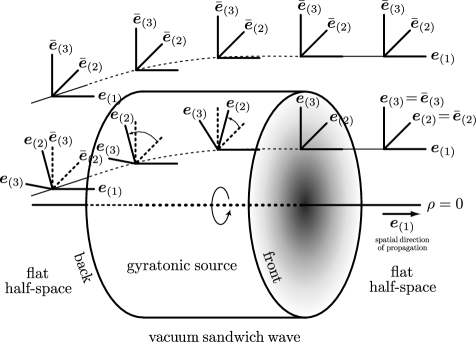
Figure 1: Schematic picture of the localized gyratonic source generating a vacuum sandwich gravitational wave. It also indicates the dragging effect which causes the parallelly propagated interpretation Cartesian frames ${\{\mbox{\boldmath$e$}_{(1)},\mbox{\boldmath$e$}_{(2)},\mbox{\boldmath$e$}_{(3)}\}}$ to rotate inside the gyraton with the angular velocity ${\dot{u}\,\omega(u,\rho,\varphi)}$ with respect to the background frames ${\{\bar{\mbox{\boldmath$e$}}_{(1)},\bar{\mbox{\boldmath$e$}}_{(2)},\bar{\mbox{\boldmath$e$}}_{(3)}\}}$. In the region outside the source it is always possible to set ${\omega=0}$.

For negligible metric functions $H$ and $a_{i}$ the metric (1) approaches flat Minkowski space with the coordinates ${u={\textstyle\frac{1}{\sqrt{2}}}(t-z)}$, ${r={\textstyle\frac{1}{\sqrt{2}}}(t+z)}$, ${x^{2}=x}$, ${x^{3}=y}$. The nontrivial gyratonic components are $T{{}_{uu}=\varrho}$ and ${T_{ui}=j_{i}}$, yielding $T{{}^{tt}=\frac{1}{2}\varrho}$, ${T^{xt}=-{\textstyle\frac{1}{\sqrt{2}}}\,j_{x}}$ and ${T^{yt}=-{\textstyle\frac{1}{\sqrt{2}}}\,j_{y}}$. Since $t$ is fixed we can substitute ${{\rm d}z}$ by ${-\sqrt{2}\,{\rm d}u}$ in which, however, the negative sign is effectively compensated by the fact that the boundary value ${z=0}$ corresponds to ${u={\textstyle\frac{1}{\sqrt{2}}}t}$ while ${z=L}$ corresponds to ${u={\textstyle\frac{1}{\sqrt{2}}}(t-L)<{\textstyle\frac{1}{\sqrt{2}}}t}$. Therefore,

$$M={\textstyle\frac{1}{\sqrt{2}}}\int\!\!\!\int\!\!\!\int\varrho\,{\rm d}x{\rm d}y{\rm d}u\,,\qquad J^{xy}=\int\!\!\!\int\!\!\!\int(yj_{x}-xj_{y})\,{\rm d}x{\rm d}y{\rm d}u\,.$$ (35)

The function

$${\cal M}(u)={\textstyle\frac{1}{\sqrt{2}}}\int\!\!\!\int_{S}\varrho\,{\rm d}x{\rm d}y\,,$$ (36)

where the surface integral is taken over the disc $S$ of radius $R$ in the transverse space, thus represents the mass-energy density of the source as a function of the retarded time $u$ such that ${M=\int\!{\cal M}(u)\,{\rm d}u}$, while the angular momentum density of the gyratonic source is given by

$${\cal J}(u)=\int\!\!\!\int_{S}(yj_{x}-xj_{y})\,{\rm d}x{\rm d}y\,,$$ (37)

so that ${J^{xy}=\int\!{\cal J}(u)\,{\rm d}u\,}$.

It is now seen from the field equation (14) that the mass-energy density ${\cal M}(u)$ of the source is determined by the metric function $H$, namely by the surface integral of ${\triangle\,H}$ in the transverse space (in the gauge ${\omega=0}$ and for ${J_{,\varphi}=0}$).

Interestingly, the angular momentum density ${\cal J}(u)$ is directly determined by the contour integral of the metric function $J$ or, equivalently, $a_{i}$. Indeed, expressing (37) in polar coordinates and employing the second field equation (13) it becomes

$${\cal J}(u)=-\int\!\!\!\int_{S}j_{\varphi}\,\rho\,{\rm d}\rho\,{\rm d}\varphi=\frac{1}{8\pi}\int_{0}^{2\pi}\!\!\Big{(}\int_{0}^{R}\omega_{,\rho}\,\rho^{2}{\rm d}\rho\Big{)}\,{\rm d}\varphi\,.$$ (38)

Using integration by parts and assuming that ${\omega\rho^{2}}$ vanishes at ${\rho=0}$, the inner integral can be rewritten as

$$\omega(R)\,R^{2}-2\int_{0}^{R}\omega\,\rho\,{\rm d}\rho\,.$$ (39)

However, ${\omega(R)=0}$ because on the cylindrical boundary ${\rho=R}$ of the gyratonic source the metric function $J$ and its derivative ${J_{,\rho}=2\omega\rho}$, cf. (9), are continuously joined to the external vacuum region in which ${\omega=0}$ everywhere (using the gauge freedom removing the rigid rotation). We thus obtain

$${\cal J}(u)=-\frac{1}{4\pi}\int\!\!\!\int_{S}\omega\,\rho\,{\rm d}\rho\,{\rm d}\varphi\,,$$ (40)

which can be reexpressed in a geometric way using expression (31) for the 2-form $\Omega$ as

$${\cal J}(u)=-\frac{1}{4\pi}\int\!\!\!\int_{S}\omega\,\rho\,\textbf{d}\rho\wedge\textbf{d}\varphi=-\frac{1}{4\pi}\int\!\!\!\int_{S}\mbox{\boldmath$\Omega$}\,.$$ (41)

Now, employing (29) and the Stokes theorem we obtain

$${\cal J}(u)=-\frac{1}{8\pi}\int\!\!\!\int_{S}\textbf{d}\mbox{\boldmath$a$}=-\frac{1}{8\pi}\oint_{C}\mbox{\boldmath$a$}\,,$$ (42)

where ${C=\partial S}$ is the outer contour. Therefore, the gauge-independent contour integral (33) directly determines the angular momentum density of the gyratonic source.

Moreover, from (41) we conclude that if ${\mbox{\boldmath$\Omega$}=0}$ everywhere in the whole spacetime, the integrals (33) vanish for any closed contour $C$ and there is no gyraton. The presence of the gyraton is identified by ${\mbox{\boldmath$\Omega$}\not=0}$ in some region, for example along (a part of) the axis. This necessarily implies ${{\cal J}(u)\not=0}$, so that the angular momentum is nonvanishing.

In particular, for the simplest gyraton [7, 8, 10, 9, 15] located at ${\rho=0}$ given by ${J=J(u)}$ only, we have ${\mbox{\boldmath$a$}=J(u)\,\textbf{d}\varphi}$ in the external vacuum region. This closed form $a$ is not globally exact, hence it can not be globally removed and ${{\cal J}(u)=-\frac{1}{4}J(u)}\not=0$ for any loop $C$ around ${\rho=0}$ as in (33). Hence, the source is gyrating.

4.3 Interpretation frame

To support this conclusion—and to enable a further analysis—it is convenient to introduce a suitable interpretation orthonormal frame ${\{\mbox{\boldmath$e$}_{a}(\tau)\}}$. At any point along an arbitrary (future-oriented) timelike geodesic ${\gamma(\tau)}$, where $\tau$ is the proper time, this defines an observer’s framework in which physical measurements are made and interpreted. The timelike vector is identified with the velocity vector of the observer, ${\mbox{\boldmath$e$}_{(0)}=\mbox{\boldmath$u$}}$, while ${\mbox{\boldmath$e$}_{(1)},\mbox{\boldmath$e$}_{(2)},\mbox{\boldmath$e$}_{(3)}}$ are perpendicular spacelike unit vectors which form its local Cartesian basis in the hypersurface orthogonal to $u$, ${\mbox{\boldmath$e$}_{a}\cdot\mbox{\boldmath$e$}_{b}\equiv g_{\alpha\beta}\,e_{a}^{\>\alpha}e_{b}^{\>\beta}=\hbox{diag}(-1,1,1,1)}$. It is also convenient to introduce an associated null frame ${\{\mbox{\boldmath$k$},\mbox{\boldmath$l$},\mbox{\boldmath$e$}_{(2)},\mbox{\boldmath$e$}_{(3)}\}}$ by the relations

$$\mbox{\boldmath$k$}={\textstyle\frac{1}{\sqrt{2}}}(\mbox{\boldmath$u$}+\mbox{\boldmath$e$}_{(1)})\,,\quad\mbox{\boldmath$l$}={\textstyle\frac{1}{\sqrt{2}}}(\mbox{\boldmath$u$}-\mbox{\boldmath$e$}_{(1)})\,.$$ (43)

Thus $k$ and $l$ are future-oriented null vectors, while $\mbox{\boldmath$e$}_{(i)}$ for ${\,i=2,3\,}$ are spatial unit vectors orthogonal to them: ${\mbox{\boldmath$k$}\cdot\mbox{\boldmath$l$}=-1}$, ${\mbox{\boldmath$e$}_{(i)}\cdot\mbox{\boldmath$e$}_{(j)}=\delta_{ij}}$, ${\mbox{\boldmath$k$}\cdot\mbox{\boldmath$k$}=0=\mbox{\boldmath$l$}\cdot\mbox{\boldmath$l$}}$, ${\mbox{\boldmath$k$}\cdot\mbox{\boldmath$e$}_{(i)}=0=\mbox{\boldmath$l$}\cdot\mbox{\boldmath$e$}_{(i)}}$. In view of definition (43), the spatial vector ${\mbox{\boldmath$e$}_{(1)}=\sqrt{2}\,\mbox{\boldmath$k$}-\mbox{\boldmath$u$}}$ is privileged, and we will refer to it as the longitudinal vector. The vectors ${\mbox{\boldmath$e$}_{(2)},\mbox{\boldmath$e$}_{(3)}}$ will be called the transverse vectors.

For the pp-wave metric (1) such an interpretation null frame, adapted to any geodesic observer with the four-velocity ${\mbox{\boldmath$u$}=\dot{r}\,\mbox{\boldmath${\partial}$}_{r}+\dot{u}\,\mbox{\boldmath${\partial}$}_{u}+\dot{x}^{2}\,\mbox{\boldmath${\partial}$}_{x^{2}}+\dot{x}^{3}\,\mbox{\boldmath${\partial}$}_{x^{3}}}$, reads

$$k \!=\! \frac{1}{\sqrt{2}\,\dot{u}}\,\mbox{\boldmath${\partial}$}_{r}\,,$$

$$l \!=\! \bigg{(}\sqrt{2}\,\dot{r}-\frac{1}{\sqrt{2}\,\dot{u}}\,\bigg{)}\,\mbox{\boldmath${\partial}$}_{r}+\sqrt{2}\,\dot{u}\,\mbox{\boldmath${\partial}$}_{u}+\sqrt{2}\,\dot{x}^{2}\,\mbox{\boldmath${\partial}$}_{x^{2}}+\sqrt{2}\,\dot{x}^{3}\,\mbox{\boldmath${\partial}$}_{x^{3}}\,,$$

$$\mbox{\boldmath$e$}_{(i)} \!=\! \bigg{(}a_{k}+\frac{\dot{x}^{j}}{\dot{u}}\delta_{jk}\bigg{)}e_{(i)}^{\>k}\,\mbox{\boldmath${\partial}$}_{r}+e_{(i)}^{\>2}\,\mbox{\boldmath${\partial}$}_{x^{2}}+e_{(i)}^{\>3}\,\mbox{\boldmath${\partial}$}_{x^{3}}\,,$$ (44)

where ${\,\delta_{kl}\,e_{(i)}^{\>k}\,e_{(j)}^{\>l}=\delta_{ij}\,}$, and the dot denotes differentiation with respect to $\tau$. In view of (2) or (2) it immediately follows that ${\dot{u}=\,}$const. along any geodesic. Notice that $k$ is proportional to the privileged null vector field $\mbox{\boldmath${\partial}$}_{r}$ which is covariantly constant. Its spatial projection is oriented along the longitudinal vector ${\mbox{\boldmath$e$}_{(1)}}$, which thus represents the propagation direction of gravitational waves and the gyratonic source, whereas ${\mbox{\boldmath$e$}_{(2)}}$, ${\mbox{\boldmath$e$}_{(3)}}$ span the transverse 2-space at any $\tau$.

Let us investigate the behaviour of the interpretation frame under the gauge (22), ${\varphi=\tilde{\varphi}+f(u)}$ with ${f_{,u}=-\omega}$, followed by the gauge (26). The latter, expressed in polar coordinates with ${\rho=\tilde{\rho}}$, takes the form ${r=\tilde{r}+g(u,\tilde{\varphi})}$, implying ${\tilde{J}=J-g_{,\tilde{\varphi}}\,}$ and ${\tilde{H}=H-2g_{,u}\,}$. Using the relations (2), (3), and taking the most convenient choice

$$e_{(2)}^{\>2}=\cos\varphi\,,\quad e_{(2)}^{\>3}=\sin\varphi\,,\qquad\qquad e_{(3)}^{\>2}=-\sin\varphi\,,\quad e_{(3)}^{\>3}=\cos\varphi$$ (45)

in (4.3), we obtain

$$k \!=\! \frac{1}{\sqrt{2}\,\dot{u}}\,\mbox{\boldmath${\partial}$}_{\tilde{r}}\,,$$ (46)

$$l \!=\! \bigg{(}\sqrt{2}\,{\dot{\tilde{r}}}-\frac{1}{\sqrt{2}\,\dot{u}}\,\bigg{)}\,\mbox{\boldmath${\partial}$}_{\tilde{r}}+\sqrt{2}\,\dot{u}\,\mbox{\boldmath${\partial}$}_{u}+\sqrt{2}\,\dot{\rho}\,\mbox{\boldmath${\partial}$}_{\rho}+\sqrt{2}\,\dot{\tilde{\varphi}}\,\mbox{\boldmath${\partial}$}_{\tilde{\varphi}}\,,$$ (47)

$$\mbox{\boldmath$e$}_{(2)} \!=\! \frac{\dot{\rho}}{\dot{u}}\,\mbox{\boldmath${\partial}$}_{\tilde{r}}+\mbox{\boldmath${\partial}$}_{\rho}\,,$$ (48)

$$\mbox{\boldmath$e$}_{(3)} \!=\! \bigg{(}\,\frac{\tilde{J}}{\rho}+\rho\,\frac{\dot{{\tilde{\varphi}}}}{\dot{u}}\,\bigg{)}\,\mbox{\boldmath${\partial}$}_{\tilde{r}}+\frac{1}{\rho}\,\mbox{\boldmath${\partial}$}_{\tilde{\varphi}}\,,$$ (49)

where

$$\tilde{J}=J-\omega\,\rho^{2}-g_{,\tilde{\varphi}}\,.$$ (50)

This gives the interpretation frame adapted to the polar coordinates of the metric (4), for which ${\,\mbox{\boldmath${\partial}$}_{\rho}\,}$ and ${\,\frac{1}{\rho}\,\mbox{\boldmath${\partial}$}_{\tilde{\varphi}}\,}$ are the natural radial and axial unit vectors in the transverse space. The form of the interpretation frame is clearly gauge invariant, with the physical part of the off-diagonal metric function determined by (50). In fact, we can always fix the most suitable gauge of coordinates (and thus the “canonical” frame) in such a way that $\tilde{J}$ does not contain the rigid rotation and the trivial part generated by the potential $g$.

For static geodesic observers with ${\dot{\rho}=0=\dot{\tilde{\varphi}}}$, the expressions (48), (49) simplify to

$$\,\mbox{\boldmath$e$}_{(2)}=\mbox{\boldmath${\partial}$}_{\rho}\,,\qquad\mbox{\boldmath$e$}_{(3)}=\frac{1}{\rho}\,(\tilde{J}\,\mbox{\boldmath${\partial}$}_{\tilde{r}}+\mbox{\boldmath${\partial}$}_{\tilde{\varphi}})\,.$$ (51)

Interestingly, the single function $\tilde{J}$ directly enters (only) the expressions (49) or (51) for the axial vector $\mbox{\boldmath$e$}_{(3)}$, distinguishing thus the usual pp-wave case ${\tilde{J}=0}$ from the case ${\tilde{J}\not=0}$ that involves the spinning gyraton source. Indeed, for the simplest gyraton [7, 10, 9] given by ${\tilde{J}=\chi(u)\not=0}$, the invariant contour integral (33) around ${\rho=0}$ gives the angular momentum density ${{\cal J}(u)=-\frac{1}{4}\,\chi(u)}$, see the end of subsection 4.2.

4.4 Analysis of the dragging effect

Now we will demonstrate that the off-diagonal metric functions $a_{i}$ in (1), or equivalently the function $J$ in (4), directly encode the rotational “dragging” effect of the spinning source on the spacetime. To this end we employ the canonical orthonormal frame ${\{\mbox{\boldmath$e$}_{a}\}}$ adapted to a (timelike) geodesic observer and the associated null frame ${\{\mbox{\boldmath$k$},\mbox{\boldmath$l$},\mbox{\boldmath$e$}_{(2)},\mbox{\boldmath$e$}_{(3)}\}}$. Using their mutual relation (43), we can prove that the interpretation null frame (4.3) is parallelly transported along a timelike geodesic $\gamma(\tau)$ in the spacetime (1) if, and only if,

$$\frac{{\rm d}e_{(i)}^{\>k}}{{\rm d}\tau}={\Omega^{\,k}}_{l}\,e_{(i)}^{\>l}\,,$$ (52)

${i,k,l=2,3\,}$, in which ${{\Omega^{\,k}}_{l}}$ are elements of the antisymmetric ${2\times 2}$ matrix

$${\Omega^{\,k}}_{l}(\tau)\equiv\dot{u}\,\delta^{kj}\,\Omega_{jl}\,,$$ (53)

where ${\,\Omega_{jl}=\frac{1}{2}(a_{l,j}-a_{j,l})}$ are the components of the 2-form ${\mbox{\boldmath$\Omega$}=\frac{1}{2}\textbf{d}\mbox{\boldmath$a$}}$, see (28), (29). The only nontrivial matrix element is ${{\Omega}^{\,2}_{\ 3}=-{\Omega}^{\,3}_{\ 2}\,}$, so that ${{\Omega}^{\,2}_{\ 3}(\tau)={\dot{u}}\,\Omega_{23}=\frac{1}{2}\,\dot{u}\,(a_{3,2}-a_{2,3})}$, evaluated along $\gamma(\tau)$, where ${\dot{u}=\,}$const. Moreover, using (2), (3), (9) we see that

$$\Omega_{23}=\frac{J_{,\rho}}{2\rho}=\omega(u,\rho,\varphi)\,.$$ (54)

To prove (52), we use the fact that the vector $k$ is covariantly constant and thus parallely transported, and therefore ${\mbox{\boldmath$l$}=\sqrt{2}\,\mbox{\boldmath$u$}-\mbox{\boldmath$k$}}$ is also parallelly transported. It only remains to ensure that $\frac{{\rm D}e_{(i)}^{\>\mu}}{{\rm d}\tau}=0$ for ${\,i=2,3\,}$. By using (4.3), (2) we obtain ${\frac{{\rm D}e_{(i)}^{\>u}}{{\rm d}\tau}=0}$. The spatial components yield the condition (52), (53). Finally, from the derivative of the condition ${\mbox{\boldmath$u$}\cdot\mbox{\boldmath$e$}_{(i)}=0\,}$ it follows that ${\,g_{\alpha\beta}\,u^{\alpha}\frac{{\rm D}e_{(i)}^{\>\beta}}{{\rm d}\tau}=0}$. Since ${\frac{{\rm D}e_{(i)}^{\>u}}{{\rm d}\tau}=0=\frac{{\rm D}e_{(i)}^{\>k}}{{\rm d}\tau}}$ we obtain ${\,g_{\alpha r}\,u^{\alpha}\frac{{\rm D}e_{(i)}^{\>r}}{{\rm d}\tau}=-\dot{u}\frac{{\rm D}e_{(i)}^{\>r}}{{\rm d}\tau}=0\Rightarrow\frac{{\rm D}e_{(i)}^{\>r}}{{\rm d}\tau}=0}$, which completes the argument (recalling that when ${\dot{u}=0}$ the geodesic cannot be timelike).

If ${\mbox{\boldmath$\Omega$}=0}$ everywhere in the spacetime, the metric functions $a_{i}$ can be globally removed by (26) and (27), hence there is no gyraton. From (52), (53) it then follows that the coefficients ${e_{(i)}^{\>k}}$ of the parallelly propagated interpretation frame are just constants. It is thus natural to consider a reference Cartesian basis ${\bar{\mbox{\boldmath$e$}}_{(2)}}$, ${\bar{\mbox{\boldmath$e$}}_{(3)}}$ given by the simplest choice ${{\bar{e}}_{(i)}^{\>k}=\delta_{i}^{k}}$. The corresponding null reference frame ${\{\mbox{\boldmath$k$},\mbox{\boldmath$l$},\bar{\mbox{\boldmath$e$}}_{(2)},\bar{\mbox{\boldmath$e$}}_{(3)}\}}$, where

$$\bar{\mbox{\boldmath$e$}}_{(i)} \!\equiv\! \bigg{(}a_{i}+\delta_{ij}\frac{\dot{x}^{j}}{\dot{u}}\bigg{)}\,\mbox{\boldmath${\partial}$}_{r}+\mbox{\boldmath${\partial}$}_{x^{i}}\,,$$ (55)

is parallelly propagated along all timelike geodesics in any non-gyratonic pp-wave spacetime and, in particular, in Minkowski background (with the usual choice ${a_{i}=0}$).

It is possible (and useful) to introduce the reference frame (55) along any geodesic in the general pp-wave spacetime with a gyraton encoded by nontrivial functions $a_{i}$. Of course, it remains parallelly propagated in the flat Minkowski regions in front and behind the sandwich/impulsive wave. Interestingly, this is also true in the vacuum region outside the gyratonic source (after removing the global rigid rotation function $\omega(u)$ by a suitable gauge (22), cf. the canonical choice allowed by (50)), as indicated in figure 1. On the other hand, inside the gyratonic source the metric components $a_{i}$ are such that ${\mbox{\boldmath$\Omega$}\not=0}$. The reference frame (55) thus does not propagate parallelly in the source region of the spacetime because the right-hand side of (52) is nonzero. Instead, it is the frame ${\{\mbox{\boldmath$k$},\mbox{\boldmath$l$},\mbox{\boldmath$e$}_{(2)},\mbox{\boldmath$e$}_{(3)}\}}$ given by (4.3) that is parallelly transported, provided (52) is satisfied.

Because both the bases ${{\bar{\mbox{\boldmath$e$}}_{(2)}},\bar{\mbox{\boldmath$e$}}_{(3)}}$ and ${\mbox{\boldmath$e$}_{(2)},\mbox{\boldmath$e$}_{(3)}}$ in the transverse 2-space are normalized to be perpendicular unit vectors, they must be related by a linear transformation

$$\mbox{\boldmath$e$}_{(i)}={A^{\,j}}_{i}\,\bar{\mbox{\boldmath$e$}}_{(j)}\,,$$ (56)

where ${\,{A^{\,j}}_{i}(\tau)\,}$ are elements of an orthonormal ${2\times 2}$ matrix. The antisymmetric matrix ${{{\Omega}^{\,k}}_{l}(\tau)}$ introduced in (53) is thus the angular velocity of rotation of the parallelly transported interpretation basis $\mbox{\boldmath$e$}_{(i)}$, given by (4.3), with respect to the reference basis $\bar{\mbox{\boldmath$e$}}_{(k)}$, introduced in (55). Indeed, for ${{\bar{e}}_{(j)}^{\>k}=\delta_{j}^{k}}$ it follows from (56) that ${e_{(i)}^{\>k}={A^{\,k}}_{i}}$. Differentiating this relation with respect to $\tau$ and using (52) we get ${\frac{{\rm d}}{{\rm d}\tau}{A^{\,k}}_{i}={\Omega^{\,k}}_{j}\,{A^{\,j}}_{i}}$. Multiplication by the inverse matrix ${{(A^{-1})^{\,i}}_{l}={(A^{T})^{\,i}}_{l}}$ yields

$${\Omega}^{\,k}_{\ l}={\big{(}\,{\textstyle\frac{{\rm d}}{{\rm d}\tau}}A\,\big{)}^{\,k}}_{i}\,{\big{(}\,A^{T}\,\big{)}^{\,i}}_{l}\,.$$ (57)

It is well known [31, 32] that this is the antisymmetric angular velocity matrix corresponding to the rotation described by $A$.

This enables us to physically interpret the metric component $J$ in the pp-wave metric (4): inside the gyratonic source it causes the “rotation dragging effect” on parallelly propagated frames, as shown in figure 1. Specifically, the parallelly transported frame (4.3) rotates in the 2-space spanned by ${\mbox{\boldmath$e$}_{(2)},\mbox{\boldmath$e$}_{(3)}}$ with the angular velocity of rotation ${{\Omega}^{\,2}_{\ 3}(\tau)={\dot{u}}\,\omega\Big{(}u(\tau),\rho(\tau),\varphi(\tau)\Big{)}}$, where ${\omega=J_{,\rho}/2\rho\,}$. Such rotation is measured with respect to the background reference frame ${\{\mbox{\boldmath$k$},\mbox{\boldmath$l$},\bar{\mbox{\boldmath$e$}}_{(2)},\bar{\mbox{\boldmath$e$}}_{(3)}\}}$, where ${\mbox{\boldmath$k$},\mbox{\boldmath$l$}}$ are the same as in (4.3) while ${\bar{\mbox{\boldmath$e$}}_{(2)},\bar{\mbox{\boldmath$e$}}_{(3)}}$ are defined in (55), which is the most natural choice when ${J=0}$.

Since we are primarily interested in impulsive or sandwich pp-waves which have compact supports (finite duration), the frames ${\bar{\mbox{\boldmath$e$}}_{(i)}}$ are well defined both “in front” and “behind” the wave, see figure 1. Moreover, when the gyratonic source is localized in a cylindrical region of radius $R$ around ${\rho=0}$, the vacuum region outside such a source globally admits the parallelly transported frame ${\{\mbox{\boldmath$k$},\mbox{\boldmath$l$},\bar{\mbox{\boldmath$e$}}_{(2)},\bar{\mbox{\boldmath$e$}}_{(3)}\}}$. It forms the reference frame of distant observers, with respect to which the parallelly transported frame (4.3) inside the source rotates.

Within the gyratonic source it follows from (13) that

$$\omega(u,\rho,\varphi)=-8\pi\int\frac{j_{\varphi}}{\rho}\,{\rm d}\rho\,.$$ (58)

At any fixed $u$ and $\varphi$, the function $\omega$ is depending on $\rho$, so that the angular velocity ${{\dot{u}}\,\omega}$ depends on the radial distance from the axis. It is thus a differential rotation which (in contrast to the rigid one) cannot be removed by a gauge. For the Bonnor solution [7] there is ${\omega\propto(R-\rho)}$ inside the cylindrical gyratonic source, i.e., $\omega$ linearly decreases to zero at its outer boundary ${\rho=R}$, and ${\omega=0}$ everywhere in the external vacuum region. This is fully consistent with the integrability conditions (28) for the 2-form ${\mbox{\boldmath$\Omega$}=\omega\,\rho\,\textbf{d}\rho\wedge\textbf{d}\varphi}$, see (31). Such conditions are obviously valid in the external vacuum region ${\rho\geq R}$, but inside the gyratonic source ${0\leq\rho<R}$ there is ${\mbox{\boldmath$\Omega$}\not=0}$, and by (41) the gyratonic source has a nonvanishing angular momentum density given by ${{\cal J}(u)\not=0}$.

4.5 The field scalars

To determine the algebraic structure of the general spacetime (4), it is important to evaluate the nontrivial Newman–Penrose scalars which are components of the gravitational and gyratonic matter fields in a suitable null frame. We employ the frame

$$k \!=\! \mbox{\boldmath${\partial}$}_{r}\,,$$ (59)

$$l \!=\! \mbox{\boldmath${\partial}$}_{u}+{\textstyle\frac{1}{2}}H\,\mbox{\boldmath${\partial}$}_{r}\,,$$ (60)

$$m \!=\! {\textstyle\frac{1}{\sqrt{2}}}(\mbox{\boldmath$e$}_{(2)}+{\rm i}\,\mbox{\boldmath$e$}_{(3)})={\textstyle\frac{1}{\sqrt{2}}}\Big{(}\,\mbox{\boldmath${\partial}$}_{\rho}+\frac{{\rm i}\,}{\rho}\,(\mbox{\boldmath${\partial}$}_{\varphi}+J\,\mbox{\boldmath${\partial}$}_{r})\Big{)}\,,$$ (61)

which is a particular case of (46)–(49) with ${\dot{\rho}=0=\dot{\varphi}}$, ${\dot{u}=\frac{1}{\sqrt{2}}}$, where we have dropped the tildes. Projecting the Weyl tensor components (using (2), (2) and ${R=0}$) we obtain

$$\Psi_{4}=-\frac{1}{4}\bigg{(}H_{,\rho\rho}-\frac{1}{\rho}H_{,\rho}-\frac{1}{\rho^{2}}H_{,\varphi\varphi}\bigg{)}-\frac{1}{2\rho^{2}}\,J_{,u\varphi}$$

$$\hskip 31.29802pt+\frac{{\rm i}\,}{2\rho^{2}}\bigg{(}\rho H_{,\rho\varphi}-H_{,\varphi}-\rho J_{,u\rho}+2J_{,u}\bigg{)}\,,$$ (62)

$$\Psi_{3}=-\frac{1}{2\sqrt{2}}\bigg{(}\,\frac{1}{\rho}\,\omega_{,\varphi}+{\rm i}\,\omega_{,\rho}\bigg{)}=-\frac{4\pi}{\sqrt{2}}\bigg{(}\,j_{\rho}-\frac{{\rm i}\,}{\rho}\,j_{\varphi}\bigg{)}\,,$$ (63)

while the nonvanishing Ricci tensor components read

$$\Phi_{22}=-\frac{1}{4}\,\triangle H+\omega^{2}+\frac{1}{2\rho^{2}}\,J_{,u\varphi}\,,$$ (64)

$$\Phi_{12}=-\bar{\Psi}_{3}\,,$$ (65)

generalizing the results presented in section 18.5 of [3]. The spacetime inside the gyratonic source is thus of Petrov type III. Notice the interesting fact that the gyrating matter component $\Phi_{12}$ is uniquely connected to the gravitational field component $\Psi_{3}$. In particular, they vanish simultaneously, so that the spacetime is of type N if, and only if, there is no gyratonic matter in the given region. In such a case, the only nontrivial Newman–Penrose scalars are $\Psi_{4}$ and $\Phi_{22}$ (representing pure radiation matter field).

Moreover, in the vacuum region outside the gyratonic source the field equations (13), (14) with ${j_{i}=0=\varrho}$ guarantee that ${\Phi_{12}=0=\Phi_{22}}$ and ${\Psi_{3}=0}$. The gravitational field is of type N with the scalar $\Psi_{4}$, which simplifies using (15)–(17) to

$$\Psi_{4}=-\frac{1}{2}\,(H_{0})_{,\rho\rho}+\frac{{\rm i}\,}{2\rho^{2}}\Big{(}\,\rho\,(H_{0})_{,\rho\varphi}-(H_{0})_{,\varphi}+2(\chi_{,u}-\omega\,\chi_{,\varphi})\Big{)}\,.$$ (66)

It can be observed that the real part of this curvature component is given by the second derivative of the function $H_{0}$ in the radial direction $\rho$, while the imaginary part is determined by its derivative in the angular direction $\varphi$ and the specific derivatives of $\chi$.

5 Geodesic deviation

Further physical properties of the gyratonic pp-wave spacetimes can be obtained by studying the specific deviation of nearby (timelike) geodesics. Such relative motion of free test particles is described by the equation of geodesic deviation [30]. To obtain invariant results, we employ the natural orthonormal frame introduced in subsection 4.3. As summarized, e.g., in [33], the geodesic deviation equation then takes the form

$$\ddot{Z}^{(\rm{i})}=R^{(\rm{i})}_{\ \>(0)(0)(\rm{j})}\,Z^{(\rm{j})}\,,$$ (67)

where ${Z^{(\rm{i})}(\tau)\equiv\mbox{\boldmath$e$}^{(\rm{i})}\cdot\mbox{\boldmath$Z$}\,}$ for ${\,\rm{i},\rm{j}=1,2,3\,}$ are spatial (Cartesian) frame components of the separation vector $\mbox{\boldmath$Z$}(\tau)$ determining the relative spatial position of two test particles, the physical relative acceleration is given by ${\ddot{Z}^{(\rm{i})}(\tau)\equiv\mbox{\boldmath$e$}^{(\rm{i})}\cdot\Big{(}\frac{{\rm D}^{2}}{{\rm d}\tau^{2}}\mbox{\boldmath$Z$}\Big{)}}$, and the relevant frame components of the Riemann tensor are ${R^{(\rm{i})}_{\ \>(0)(0)(\rm{j})}=R_{(\rm{i})(0)(0)(\rm{j})}\equiv R_{\mu\alpha\beta\nu}\,e^{\mu}_{(\rm{i})}u^{\alpha}u^{\beta}e^{\nu}_{(\rm{j})}}$.

In view of (4) with (18), the only nontrivial components ${R_{(\rm{i})(0)(0)(\rm{j})}}$ in the reference frame (46)–(49) where ${\mbox{\boldmath$e$}_{(0)}=\mbox{\boldmath$u$}={\textstyle\frac{1}{\sqrt{2}}}(\mbox{\boldmath$k$}+\mbox{\boldmath$l$})}$, simplified by the gauge (22), (26), are ${R_{(2)(0)(0)(2)}=-R_{(3)(0)(0)(3)}\equiv{\cal A}_{+}}$, ${R_{(2)(0)(0)(3)}\equiv{\cal A}_{\times}}$, in which

$${\cal A}_{+} \!=\! \frac{1}{2}\,\dot{u}^{2}\,(H_{0})_{,\rho\rho}\,,$$

$${\cal A}_{\times} \!=\! \frac{1}{2}\,\dot{u}^{2}\frac{1}{\rho^{2}}\Big{(}\,\rho\,(H_{0})_{,\rho\varphi}-(H_{0})_{,\varphi}+2(\chi_{,u}-\omega\,\chi_{,\varphi})\Big{)}\,.$$ (68)

Recall that ${\omega=0}$ in the vacuum region outside the gyratonic source. The invariant equation of geodesic deviation (67) in the interpretation frame, evaluated along the chosen timelike geodesic ${\gamma(\tau)}$, thus takes the explicit form

$$\ddot{Z}^{(1)} \!=\! 0\,,$$

$$\ddot{Z}^{(2)} \!=\! {\cal A}_{+}\,Z^{(2)}+{\cal A}_{\times}\,Z^{(3)}\,,$$ (69)

$$\ddot{Z}^{(3)} \!=\! {\cal A}_{\times}\,Z^{(2)}-{\cal A}_{+}\,Z^{(3)}\,,$$

where the functions ${{\cal A}_{+}}$ and ${{\cal A}_{\times}}$ obviously determine the two “+” and “$\times$” polarization amplitudes of the transverse gravitational waves propagating along ${\mbox{\boldmath$e$}_{(1)}}$, respectively.

It is now straightforward to calculate the explicit forms of these wave amplitudes for the large family of exact solutions (3) when ${\chi=\chi(u)}$:

$${\cal A}_{+} \!=\! \dot{u}^{2}\,\Bigg{[}\,\frac{\mu(u)}{\rho^{2}}\hskip 8.53581pt+\frac{1}{2}\sum_{m=1}^{\infty}m(m+1)\,\frac{B_{m}(u)}{\rho^{m+2}}\,\cos\Big{[}m\Big{(}\varphi-\varphi_{m}(u)\Big{)}\Big{]}$$ (70)

$$\hskip 60.60437pt+\frac{1}{2}\sum_{m=2}^{\infty}m(m-1)\,A_{m}(u)\,\rho^{m-2}\cos\Big{[}m\Big{(}\varphi-\varphi^{\prime}_{m}(u)\Big{)}\Big{]}\Bigg{]}\,,$$

$${\cal A}_{\times} \!=\! \dot{u}^{2}\,\Bigg{[}\,\frac{\chi_{,u}(u)}{\rho^{2}}+\frac{1}{2}\sum_{m=1}^{\infty}m(m+1)\,\frac{B_{m}(u)}{\rho^{m+2}}\,\sin\Big{[}m\Big{(}\varphi-\varphi_{m}(u)\Big{)}\Big{]}$$ (71)

$$\hskip 60.60437pt-\frac{1}{2}\sum_{m=2}^{\infty}m(m-1)\,A_{m}(u)\,\rho^{m-2}\sin\Big{[}m\Big{(}\varphi-\varphi^{\prime}_{m}(u)\Big{)}\Big{]}\Bigg{]}\,.$$

The first terms $\mu$ and $\chi_{,u}$ in each amplitude represent the gravitational field of axially symmetric “extended” Aichelburg–Sexl solution [24, 25] with an ultrarelativistic monopole gyratonic source located along the axis ${\rho=0}$, which we will describe in more detail in the next subsection 5.1. The terms $B_{m}$ correspond to asymptotically flat pp-wave solutions with multipole gyratonic sources located along ${\rho=0}$ [26, 27, 10, 28]. For example, the gyrating dipole source is given by the profile function $B_{1}$ and $\chi_{,u}$. The gravitational field of the plane wave is described by $A_{2}$, in which case the wave amplitudes ${\cal A}_{+}$ and ${\cal A}_{\times}$ are independent of the radial coordinate $\rho$. Non-homogeneous pp-waves with directional curvature singularities at ${\rho=\infty}$ (where ${{\cal A}_{+}}$, ${{\cal A}_{\times}}$ diverge) are given by higher-order terms $A_{m}$ with ${m=3,4,\ldots}$ [20, 21, 22, 23]. With ${\chi_{,u}\not=0}$ we obtain their gyrating versions which manifest themselves in the amplitude ${\cal A}_{\times}$ of geodesic deviation (5).

5.1 The axially symmetric case

The simplest vacuum pp-wave solution with a gyratonic source is the axially symmetric one. It can be written in the form (4) with the metric functions (24) and (25) independent of the angular coordinate $\varphi$. Since the only axially symmetric solution of (18) is ${H=H_{0}=-2\,\mu(u)\,\log\rho}$, see (3), we are thus left with

$$J(u)=\chi(u)\,,\qquad H(u,\rho)=-2\,\mu(u)\,\log\rho\,.$$ (72)

The case ${\,J=0\,}$ represents the “extended” Aichelburg–Sexl solution because in the distributional limit when ${\mu(u)\to\delta(u)}$ we obtain the spacetime [24] describing the specific impulsive gravitational wave generated by a nonrotating ultrarelativistic monopole point source located at ${\rho=0=u}$.

The case ${\,J\not=0\,}$ describes the Frolov–Fursaev gyraton investigated in [9]. There is a curvature singularity at ${\rho=0}$ whenever ${\mu\not=0}$. This can be immediately seen from the gravitational wave amplitudes (70), (71), which for (72) simplify considerably to

$${\cal A}_{+}=\dot{u}^{2}\,\frac{\mu}{\rho^{2}}\,,\qquad{\cal A}_{\times}=\dot{u}^{2}\,\frac{\chi_{,u}}{\rho^{2}}\,.$$ (73)

Moreover, we conclude that the functions $\mu(u)$ and $\chi_{,u}(u)$ directly determine the “+” and “$\times$” polarization amplitudes of the gravitational waves, respectively, as seen by the transverse deviations (5) between the geodesic observers. Interestingly, both these physically relevant functions in the metric coefficients $H$ and $J$ (determining the energy and angular momentum density of the null source) are thus directly observable by a detector of gravitational waves as the disctinct polarization states. For the non-spinning Aichelburg–Sexl source, the corresponding gravitational pp-wave is purely “+” polarized since in the case ${\chi_{,u}=0}$ there is ${{\cal A}_{\times}=0}$.

Notice that for (72) the mass-energy density (36) of the source can be explicitly evaluated. Using (14) we obtain ${\varrho=-\frac{1}{16\pi}\triangle\,H=\frac{1}{8\pi}\,\mu\,\triangle\,\log\rho=\frac{1}{4}\,\mu\,\delta^{(2)}}$, so that

$${\cal M}(u)={\textstyle\frac{1}{4\sqrt{2}}}\,\mu(u)\,.$$ (74)

The metric function $\mu(u)$ thus directly determines the mass-energy density ${\cal M}(u)$ of the gyratonic source. Since the source propagates with the speed of light, its rest mass must be zero which means that ${{\cal M}(u)=\frac{1}{4\sqrt{2}}\,\mu(u)}$ also equals to the density of momentum while ${{\cal J}(u)=-\frac{1}{4}\,\chi(u)}$ is the density of angular momentum of the gyraton.

6 Geodesics

In this part we are going to analyze geodesics ${u\not=\,}$const. in gyratonic pp-waves. Since all Christoffel symbols (2) of the form $\Gamma^{u}_{\alpha\beta}$ vanish we may choose $u$ as an affine parameter. Setting $\dot{u}=1$ we arrive at the following set of equations for the metric (4):

$$\ddot{r}-\frac{1}{2}H_{,u}+\frac{1}{2\rho^{2}}J(2J_{,u}-H_{,\varphi})-(H_{,\rho}-\frac{1}{\rho^{2}}JJ_{,\rho})\dot{\rho}-H_{,\varphi}\dot{\varphi}+\frac{1}{\rho}(2J-\rho J_{,\rho})\dot{\rho}\,\dot{\varphi}-J_{,\varphi}\dot{\varphi}^{2}=0\,,$$

$$\ddot{\rho}-\rho\,\dot{\varphi}^{2}-\frac{1}{2}H_{,\rho}-J_{,\rho}\,\dot{\varphi}=0\,,$$ (75)

$$\ddot{\varphi}+\frac{2}{\rho}\,\dot{\rho}\,\dot{\varphi}+\frac{1}{2\rho^{2}}\,(2J_{,u}-H_{,\varphi})+\frac{1}{\rho^{2}}\,J_{,\rho}\,\dot{\rho}=0\,,$$

where ${\dot{\,}=\frac{{\rm d}}{{\rm d}u}\,}$. The equation for $r$ is clearly decoupled and can be simply integrated once the rest of the system has been solved. Applying the vacuum field equations and the gauge leading to the form (24), (25), the transverese part simplifies to

$$\ddot{\rho}-\rho\,\dot{\varphi}^{2}-\frac{1}{2}H_{0,\rho}=0\,,\qquad\ddot{\varphi}+\frac{2}{\rho}\,\dot{\rho}\,\dot{\varphi}+\frac{1}{\rho^{2}}\Big{(}\chi_{,u}-\frac{1}{2}H_{0,\varphi}\Big{)}=0\,.$$ (76)

In the case of axial symmetry, by (72) the equations further reduce to

$$\ddot{\rho}-\rho\,\dot{\varphi}^{2}+\frac{\mu}{\rho}=0\,,\qquad\ddot{\varphi}+\frac{2}{\rho}\,\dot{\rho}\,\dot{\varphi}+\frac{\chi_{,u}}{\rho^{2}}=0\,.$$ (77)

We observe that the mass-energy density proportional to $\mu(u)$ only occurs in the radial $\rho$-equation, while the derivative $\chi_{,u}$ of the angular momentum density proportional to $\chi(u)$ only appears in the $\varphi$-equation. An analysis of (77) as in [10] shows that positive energy qualitatively exerts an attractive force which leads to a focussing effect of the geodesics. On the other hand, angular momentum exerts a rotational effect on the geodesics. Note that we have already encountered the analogous separation of effects in the geodesic deviation amplitudes (73). Due to the axial symmetry we also have a conserved quantity $\chi_{0}$ associated with the Killing vector $\partial_{\varphi}$ which enables us to rewrite the equations (77) as

$$\ddot{\rho}=-\frac{\mu(u)}{\rho}+\frac{[\,\chi_{0}-\chi(u)]^{2}}{\rho^{3}}\,,\qquad\dot{\varphi}=\frac{\chi_{0}-\chi(u)}{\rho^{2}}\,.$$ (78)

The first term in the equation for radial acceleration $\ddot{\rho}$ represents the focussing due to the positive energy density $\mu(u)$ of the source, while the second term is the nonlinear coupling to its angular momentum. The equation for the speed of rotation $\dot{\varphi}$ clearly involves the influence of the angular momentum density of the source ${{\cal J}(u)}$ proportional to $\chi(u)$, effectively adding to the conserved quantity $\chi_{0}$.

7 Impulsive limit

In [9, 10] impulsive versions of gyratons have been introduced along with their extended versions and have been used prominently in [15]. Here we give a somewhat broader discussion of possible impulsive limits in the class of gyratonic pp-wave spacetimes. We consider the vacuum line element (4) with (24), (25), that is

$${\rm d}s^{2}={\rm d}\rho^{2}+\rho^{2}\,{\rm d}\varphi^{2}-2\,{\rm d}u\,{\rm d}r+2\,\chi(u,\varphi)\,{\rm d}u\,{\rm d}\varphi+H_{0}(u,\rho,\varphi)\,{\rm d}u^{2}\,,$$ (79)

where $\chi(u,\varphi)$ is an arbitrary function while $H_{0}(u,\rho,\varphi)$ is a solution of (17). There are now two distinct cases that have to be treated separately.

7.1 The case ${\Sigma=0}$

With the constraint ${\Sigma(u,\varphi)\equiv 2(\chi_{,u\varphi}-\omega\,\chi_{,\varphi\varphi})=0}$, the remaining vacuum field equation reduces to the Laplace equation ${\triangle\,H_{0}=0}$. In the natural global gauge ${\omega=0}$, the constraint implies that the function $\chi_{,u}$ is independent of $\varphi$, so that ${\chi(u,\varphi)=\chi(u)+\Phi(\varphi)}$. In such a case we see that the field equations put no restriction on the $u$-dependence of $H_{0}$ and $\chi$. In analogy with the usual (non-gyratonic) class of sandwich and impulsive pp-waves in Minkowski space (and corresponding models with a nonvanishing cosmological constant [28, 29]) we now consider the metric functions of the form

$$H_{0}(u,\rho,\varphi)=\tilde{H}_{0}(\rho,\varphi)\,\chi_{H}(u)\,,\qquad\chi(u,\varphi)=J(u,\varphi)=\tilde{\chi}\,\chi_{J}(u)+\Phi(\varphi)\,,$$ (80)

where $\tilde{\chi}$ is a constant and we call the functions $\chi_{H}(u)$ and $\chi_{J}(u)$ profile functions of the energy and angular momentum densities, respectively. Here we assume $\int\!\chi_{H}(u)\,{\rm d}u=1=\int\!\chi_{J}(u)\,{\rm d}u$ but otherwise these functions are completely arbitrary. In particular, these profiles can be choosen independently of each other — we have a complete separation of $\chi_{H}(u)$ and $\chi_{J}(u)$. From (4) it then follows that

$$R_{u\rho u\rho}=-\frac{1}{2}(\tilde{H}_{0})_{,\rho\rho}\,\chi_{H}(u)\,,$$

$$R_{u\rho u\varphi}=-\frac{1}{2\rho}\Big{(}\rho\,(\tilde{H}_{0})_{,\rho\varphi}-(\tilde{H}_{0})_{,\varphi}\Big{)}\,\chi_{H}(u)-\frac{\tilde{\chi}}{\rho}\,{\chi_{J}}_{,u}(u)\,,$$ (81)

$$R_{u\varphi u\varphi}=-\frac{1}{2}\Big{(}(\tilde{H}_{0})_{,\varphi\varphi}+\rho(\tilde{H}_{0})_{,\rho}\Big{)}\,\chi_{H}(u)\,,$$

which in the axisymmetric case (72) with ${\chi_{H}(u)=\mu(u)}$ and ${\chi(u)=\tilde{\chi}\,\chi_{J}(u)}$ reduce to

$$R_{u\rho u\rho}=-\frac{1}{\rho^{2}}\,\mu(u)\,,\quad R_{u\rho u\varphi}=-\frac{1}{\rho}\,\chi_{,u}(u)\,,\quad R_{u\varphi u\varphi}=\mu(u)\,.$$ (82)

We thus observe, that the energy profile $\chi_{H}(u)$ explicitly shows up in the curvature, and so does the angular momentum profile $\chi_{J}(u)$ in term of its derivative ${\chi_{J}}_{,u}(u)$. This is in accordance with (5) where the energy profile determines the amplitude ${\cal A}_{+}$, while the angular momentum profile determines the amplitude ${\cal A}_{\times}$, which then also contains the derivative of the profile. The same effect becomes visible in the only nonvanishing field scalar $\Psi_{4}$ (66), which in the axially symmetric case takes the form

$$\Psi_{4}=-\frac{1}{\rho^{2}}\,\mu(u)+\frac{{\rm i}\,}{\rho^{2}}\,\chi_{,u}(u)\,.$$ (83)

All this suggests that — in accordance with the usual definition of impulsive waves — one may take the energy profile $\chi_{H}(u)$ to be $\delta$-shaped (the Dirac $\delta$ distribution) but one should rather confine oneself with a box-like profile for the angular momentum $\chi_{J}(u)$. Indeed, a $\delta$-shaped angular momentum profile would introduce a $\delta^{\prime}$-term in the curvature, the amplitude ${\cal A}_{\times}$ and the filed scalar $\Psi_{4}$. This seems to be less physical.

Indeed in [9] such a box-shaped profile for both energy and angular momentum densities was considered, i.e., ${\chi_{H}(u)=\chi_{J}(u)=\vartheta_{L}(u)}$ where

$$\vartheta_{L}(u)\equiv\frac{1}{L}\Big{(}\Theta(u)-\Theta(u-L)\Big{)}\,,$$ (84)

in which ${L>0}$ is the “length” of the profile and $\Theta$ denotes the Heaviside step function, see the left part of figure 2.

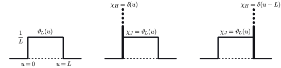
Figure 2: Schematic representation of possible profiles $\chi_{H}(u)$ for energy and $\chi_{J}(u)$ for angular momentum densities: a box-shaped profile $\vartheta_{L}(u)$ for both $\chi_{H}$ and $\chi_{J}$ (left); the choice ${\chi_{H}=\delta(u)}$ with ${\chi_{J}=\vartheta_{L}(u)}$ (middle); alternative choice ${\chi_{H}=\delta(u-L)}$ with ${\chi_{J}=\vartheta_{L}(u)}$ (right).

In [15] the energy profile was changed to be impulsive, more precisely ${\chi_{H}(u)=\delta(u)}$, as shown in the middle part of figure 2, or alternatively ${\chi_{H}(u)=\delta(u-L)}$, see the right part of figure 2. This is possible since arbitrary and independent profile functions $\chi_{H}(u)$ and $\chi_{J}(u)$ can be prescribed in the ${\Sigma=0}$ case.

7.2 The case ${\Sigma\not=0}$

If the metric function ${J=\chi(u,\varphi)}$ nontrivially depends on the angular coordinate $\varphi$ then ${\Sigma\not=0}$ and the field equations naturally lead to a coupling of the profiles. More precisely, the vacuum equation (17) with ${\omega=0}$ then reduces to

$$\triangle H_{0}(u,\rho,\varphi)=\frac{2}{\rho^{2}}\ \chi_{,u\varphi}(u,\varphi),$$ (85)

and the splitting generalizing (80) to admit ${\tilde{\chi}=\tilde{\chi}(\varphi)}$,

$$H_{0}(u,\rho,\varphi)=\tilde{H}_{0}(\rho,\varphi)\,\chi_{H}(u)\,,\qquad\chi(u,\varphi)=\tilde{\chi}(\varphi)\,\chi_{J}(u)+\Phi(\varphi)\,,$$ (86)

gives

$$\triangle\tilde{H}_{0}(\rho,\varphi)\,\chi_{H}(u)=\frac{2}{\rho^{2}}\ \tilde{\chi}_{,\varphi}(\varphi)\,{\chi_{J}}_{,u}(u)\,.$$ (87)

If the supports of $\chi_{H}(u)$ and $\chi_{J}(u)$ are disjoint, then separately ${\triangle\tilde{H}_{0}=0}$ and ${\tilde{\chi}_{,\varphi}=0}$, implying ${\Sigma=0}$. Thus, for solutions with ${\Sigma\not=0}$, both the supports must agree, in which case the box profile (84) in the angular momentum density, ${\chi_{J}(u)=\vartheta_{L}(u)}$, naturally leads to two Dirac deltas in the energy density, namely ${\chi_{H}(u)=\delta(u)-\delta(u-L)}$ (to satisfy the relation ${\chi_{H}(u)\propto{\chi_{J}}_{,u}(u)}$ in (87)), see the left part of figure 3. Assuming (86) we thus obtain an impulse in energy on each edge of the box, one positive and the other negative. Hence, the energy distribution in such a gyratonic source would have a dipole character. Moreover, the corresponding spatial Poisson equation

$$\triangle\tilde{H}_{0}(\rho,\varphi)=\frac{2}{L}\,\frac{\tilde{\chi}_{,\varphi}(\varphi)}{\rho^{2}}\,,$$ (88)

also has to be solved.

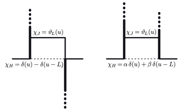
Figure 3: Possible profiles $\chi_{H}(u)$ for energy density in the case of a general $\Sigma$ and the box-shaped angular momentum profile ${\chi_{J}(u)=\vartheta_{L}(u)}$: the natural choice ${\chi_{H}=\delta(u)-\delta(u-L)}$ (left); more general choice ${\chi_{H}=\alpha\,\delta(u)+\beta\,\delta(u-L)}$ (right).

The drawback of the particular solution ${\chi_{H}(u)=\delta(u)-\delta(u-L)}$ is that it involves a negative energy distribution located at ${u=L}$. However, physically more relevant solutions can be constructed by superimposing this particular solution with specific homogeneous solutions proportional to a positive profile $\delta(u-L)$ (and also possibly $\delta(u)$), effectively leading to a general energy density profile function ${\chi_{H}=\alpha\,\delta(u)+\beta\,\delta(u-L)}$ with positive parameters $\alpha$ and $\beta$, see the right part of figure 3.

In fact, as suggested by the referee, more general solution of the linear equation (85) takes the form ${H_{0}=H_{0}^{(h)}(u,\rho,\varphi)+H_{0}^{(p)}(u,\rho,\varphi)}$, where ${\triangle H_{0}^{(h)}=0}$ and ${\triangle H_{0}^{(p)}=2\rho^{-2}\chi_{,u\varphi}\,}$ with the additional requirement

$$\oint H_{0}^{(p)}(u,\rho,\varphi)\,{\rm d}\varphi=0\,.$$ (89)

The corresponding energy profiles ${\chi_{H}^{(h)}(u)}$ and ${\chi_{H}^{(p)}(u)}$ are independent. We can choose ${\chi_{H}^{(h)}(u)}$ in such a way that the energy is positive (the case ${\Sigma=0}$). Due to the additional constraint (89) the energy of the complete solution ${H_{0}=H_{0}^{(h)}+H_{0}^{(p)}}$ remains positive because the contribution from ${H_{0}^{(p)}}$ becomes zero after the $\varphi$-integration.

8 Completeness of geodesics in the impulsive limit

Finally, we analyze the geodesic equations in the impulsive limit of the ${\Sigma=0}$ case, i.e., the models extending those of [15], also discussed in subsection 7.1. Specifically, we consider the metric (79), (80) with

$$\chi_{H}(u)=\alpha\,\delta(u)+\beta\,\delta(u-L)\,,\qquad\chi_{J}(u)=\vartheta_{L}(u)\,,$$ (90)

where the box-profile ${\vartheta_{L}(u)}$ is defined in (84) and $\alpha$, $\beta$ are arbitrary real parameters, indicated in the right part of figure 3. They enable us to set the respective impulsive components to any values (including turning them off). Using (76) we find that the spatial part of the geodesic equations takes the form

$$\ddot{\rho}-\rho\,\dot{\varphi}^{2}-\frac{1}{2}\,\tilde{H}_{0,\rho}(\rho,\varphi)\Big{(}\alpha\,\delta(u)+\beta\,\delta(u-L)\Big{)}=0\,,$$ (91)

$$\ddot{\varphi}+\frac{2}{\rho}\,\dot{\rho}\,\dot{\varphi}+\frac{1}{\rho^{2}}\,\frac{\tilde{\chi}}{L}\Big{(}\delta(u)+\delta(u-L)\Big{)}-\frac{1}{2\rho^{2}}\tilde{H}_{0,\varphi}(\rho,\varphi)\Big{(}\alpha\,\delta(u)+\beta\,\delta(u-L)\Big{)}=0\,.$$ (92)

These equations have a form similar to the geodesic equations in impulsive NP-waves, which have recently been analyzed rigorously in [34, 35]. This is best seen by looking at the geodesic equations in Cartesian coordinates $x^{i}$ of the metric (1), which using (2) are

$${\textstyle\ddot{x}^{i}+\delta^{ij}(a_{j,u}-\frac{1}{2}H_{,j})+\delta^{ik}(a_{k,j}-a_{j,k})\,\dot{x}^{j}=0}\,.$$ (93)

In view of (3), in the present case they are of the form

$$\ddot{x}(u)+G_{1}(x)\,\delta(u)+G_{2}(x)\,\delta(u-L)+G_{3}(x,\dot{x})\,\vartheta_{L}(u)=0\,,$$ (94)

where for simplicity we have collected all dependencies on the spatial variables ${x=(x^{2},x^{3})}$, spanning the transverse plane, in the functions ${G_{1},G_{2},G_{3}}$. In particular, assuming these functions to be smooth, the technical result derived in [34, Lem. A.2] (with minor modifications, namely replacing $F_{1}(x_{\epsilon},\dot{x}_{\epsilon})$ by $F_{1}(x_{\epsilon},\dot{x}_{\epsilon})\Theta_{\epsilon}$) also applies in the present situation and we obtain a completeness result. More precisely, if one regularizes the profile functions replacing $\delta$ by a standard mollifier ${\delta_{\epsilon}(x)\equiv(1/\epsilon)\,\phi(x/\epsilon)}$ ($\phi$ a smooth function supported in $[-1,1]$ with unit integral) and replacing $\Theta$ by ${\Theta_{\epsilon}(x)\equiv\int_{-1}^{x}\phi_{\epsilon}(t)\,{\rm d}t}$ one obtains the following completeness statement: For any geodesic starting long before the shock, say at $u=-1$, there exists an $\epsilon_{0}$ such that it passes the shock region ${u\in[0,L]}$ provided ${\epsilon\leq\epsilon_{0}}$. The geodesics will be straight lines up to ${u=0}$ where they will be refracted with their $r$-component suffering an additional jump. During the support of the angular momentum profile ${u\in[0,L]}$ an angular motion is excerted. Another break occurs at ${u=L}$ and after that the geodesics return to be straight lines.

In the more realistic case where the ${G_{1},G_{2},G_{3}}$ are non-smooth on the axis ${\rho=0}$ (including the Aichelburg–Sexl solution) the result still applies with the exception of those geodesics which are directly heading into the curvature singularity at ${u=0}$, ${\rho=0}$ and those which are refracted to directly hit the singularity at ${u=L}$, ${\rho=0}$. A more detailed analysis of the geodesic motion in these and more general models is subject to current research.

9 Conclusions

We have studied the complete family of pp-waves with flat wavefronts in Einstein’s general relativity. Thereby we have kept all terms in the original Brinkmann form of the metric (1), in particular, the off-diagonal ones ${a_{i}(u,x^{j})\,{\rm d}u\,{\rm d}x^{i}}$. In almost all prior investigations of this famous family of exact spacetimes the functions $a_{2}$ and $a_{3}$ have been ignored because (in any vacuum region) it is always possible locally to set ${a_{i}=0}$ by a suitable gauge. However, it was only Bonnor in 1970 and independently Frolov and his collaborators in 2005 who pointed out the physical significance of these off-diagonal terms. In general, they cannot be removed globally, and in such a case they encode angular momentum. For a localized matter distribution the spacetime metric can be interpreted as the gravitational field of a spinning source moving at the speed of light, called gyraton [9, 10]. Here we have significantly extended and complemented the previous studies [7, 9, 10, 15] explicitly investigating various mathematical, geometrical and physical properties of these spacetimes.

We have fully integrated the vacuum Einstein equations in section 3, yielding the general metric functions $J$ and $H$, see (15) and (16). Then we have used the complete gauge freedom to understand the geometrical and physical meaning of all the integration functions $\omega(u)$, $\chi(u,\varphi)$ and $H_{0}(u,\rho,\varphi)$. We showed that the function $\omega(u)$ represents angular velocity of a rigid rotation of the whole spacetime, which can always be set to zero in the vacuum region by using (22). With ${\omega=0}$ it is then possible to employ the second gauge (26) to set the function ${J=\chi(u,\varphi)}$ to zero since the integrability conditions ${\mbox{\boldmath$\Omega$}=\frac{1}{2}\,J_{,\rho}\,\textbf{d}\rho\wedge\textbf{d}\varphi=0}$ are satisfied, see (31), (32). However, this can be done only locally. In fact, the key $2$-form $\Omega$ is given by ${\mbox{\boldmath$\Omega$}=\frac{1}{2}\,\textbf{d}\mbox{\boldmath$a$}}$, where ${\mbox{\boldmath$a$}\equiv a_{i}\,\textbf{d}x^{i}}$, cf. (29), and in general the closed $1$-form $a$ need not be globally exact. This happens, in particular, if a gyratonic source is located along the axis ${\rho=0}$, so that the external vacuum region is not contractible. Then it is necessary to keep the off-diagonal metric terms even in the vacuum region.

Moreover, as shown in [7, 9] and subsection 4.2, the function $H$ is related to the mass-energy density ${\cal M}(u)$ while $J$ encodes the angular momentum density ${\cal J}(u)$ of the gyratonic source via the gauge-independent contour integral ${{\cal J}(u)=-\frac{1}{8\pi}\oint_{C}\mbox{\boldmath$a$}=-\frac{1}{8\pi}\oint_{C}J\,\textbf{d}\varphi}$, cf. (42), (33). This yields a clear physical interpretation of the metric functions.

To analyze further aspects of the gyratonic sources represented by the metric functions $a_{i}$ that have not been studied before, we introduced in subsection 4.3 a natural orthonormal frame for any geodesics observer and its associated null frame (4.3). After studying their gauge freedom, in subsection 4.4, we analyzed the rotational dragging effect of parallelly propagated frames caused by the spinning gyratonic matter. Specifically, we proved that the angular velocity of the spatial rotation of such frames is given by ${{\Omega}^{\,2}_{\ 3}={\dot{u}}\,\omega(u,\rho,\varphi)}$, where ${\omega=\frac{1}{2}J_{,\rho}/\rho=\frac{1}{2}(a_{3,2}-a_{2,3})}$ is the only nontrivial component of the key 2-form $\Omega$. Therefore, in the external vacuum region there is no such dragging while inside the gyratonic source, where ${\mbox{\boldmath$\Omega$}\not=0}$, we have rotation of frames, see figure 1.

In subsection 4.5 we analyzed the Newman–Penrose scalars (62)–(65). The spacetime inside the source is of Petrov type III, with the gyrating matter component $\Phi_{12}$ coupled to the gravitational component $\Psi_{3}$ so that they (do not) vanish simultaneously. The gravitational field in the exterior vacuum region is thus of type N with $\Psi_{4}$ given by (66).

As a further new application of the interpretation frame, in section 5 we investigated the invariant form of the geodesic deviation. This allows to clearly separate the longitudinal direction, in which the gravitational wave propagates, and the transverse 2-space where its effect on relative motion of test particles is observed (5). We explicitly evaluated the two polarization amplitudes ${{\cal A}_{+}}$ and ${{\cal A}_{\times}}$, see (5), which turn out to be proportional to the real and the imaginary part of $\Psi_{4}$, respectively. In the axisymmetric case with ${J=\chi(u)}$, ${H=-2\,\mu(u)\,\log\rho}$ (the Frolov–Fursaev gyraton constructed from the Aichelburg–Sexl solution), which we have studied in subsection 5.1, the amplitudes are given by ${{\cal A}_{+}=\mu\,\dot{u}^{2}\rho^{-2}}$ and ${{\cal A}_{\times}=\chi_{,u}\,\dot{u}^{2}\rho^{-2}}$. Interestingly, both physical profile functions $\mu(u)$ and $\chi(u)$ of $H$ and $J$ (determining the energy and angular momentum densities) are thus observable by a detector of gravitational waves as distinct “+” and “$\times$” polarization states, with the wave being purely “+” polarized in the absence of a gyraton. It follows from (70), (71) that a similar behavior also occurs for non-axisymmetric gyratons with multipole sources.

It is important to observe that it is the derivative $\chi_{,u}$ of the metric function ${J=\chi(u,\varphi)}$ which appears in the curvature $\Psi_{4}$ and in the wave amplitude ${\cal A}_{\times}$. Moreover, $\chi_{,u}$ directly influences the behavior of geodesics, studied in section 6, namely the axial acceleration $\ddot{\varphi}$. On the other hand, the mass-energy density of the gyraton encoded in ${H=H_{0}(u,\rho,\varphi)}$ determines the radial acceleration $\ddot{\rho}$, causing a focusing of the geodesics.

We have studied impulsive limits of gyratonic pp-waves in section 7. There we emphasized that (unlike in previous works) it is necessary to distinguish the cases $\Sigma=0$ and $\Sigma\not=0$, when solving the Poisson equation (17). If ${\Sigma=0}$ it reduces to the Laplace equation and the field equations put no restriction on the $u$-dependence of $H_{0}$ and $J$. Hence the corresponding profiles $\chi_{H}(u)$ and $\chi_{J}(u)$ of the energy and the angular momentum densities can be chosen independently of each other. Since by (7.1) the curvature is proportional to $\chi_{H}$ and ${\chi_{J}}_{,u}$, it is natural to consider impulsive waves by setting the profile $\chi_{H}(u)$ to be proportional to the Dirac $\delta$ but using a box-like profile $\vartheta_{L}(u)$ for $\chi_{J}(u)$, see (84) and figure 2.

On the other hand, when $\Sigma\not=0$ the supports of $\chi_{H}(u)$ and ${\chi_{J}}_{,u}(u)$ must coincide. In particular, the box $\vartheta_{L}(u)$ in the angular momentum density profile $\chi_{J}(u)$ naturally leads to two Dirac deltas in the energy density, ${\chi_{H}=\delta(u)-\delta(u-L)}$. These two (opposite) impulses on each edge of the box are shown in the left part of figure 3. Physically more relevant solutions can be constructed by superimposing such a particular solution with specific homogeneous solutions. This effectively leads to a general energy density profile ${\chi_{H}=\alpha\,\delta(u)+\beta\,\delta(u-L)}$ with positive parameters $\alpha$ and $\beta$, see the right part of figure 3.

In the final section 8 we analyzed the geodesic equations in the impulsive limit. We considered the ${\Sigma=0}$ case and the generic profiles ${\chi_{H}=\alpha\,\delta(u)+\beta\,\delta(u-L)}$ and ${\chi_{J}=\vartheta_{L}(u)}$ where $\alpha$, $\beta$ are arbitrary constants. We showed that any geodesic starting long before such a wave passes the shock region ${u\in[0,L]}$, considering regularizations of the Dirac deltas and the box by standard smooth mollifiers. In other words, we proved geodesic completeness of impulsive gyratonic pp-wave spacetimes.

References

- [1] H. W. Brinkmann, Einstein spaces which are mapped conformally on each other, Math. Ann. 94, 119–45 (1925).
- [2] H. Stephani, D. Kramer, M. MacCallum, C. Hoenselaers and E. Herlt, Exact Solutions of Einstein’s Field Equations (Cambridge University Press, Cambridge, 2003).
- [3] J. B. Griffiths and J. Podolský, Exact Space-Times in Einstein’s General Relativity (Cambridge University Press, Cambridge, 2009).
- [4] V. Pravda, A. Pravdová, A. Coley and R. Milson, All spacetimes with vanishing curvature invariants, Class. Quantum Grav. 19, 6213–36 (2002).
- [5] A. Coley, G. W. Gibbons, S. Hervik and C. N. Pope, Metrics with vanishing quantum corrections, Class. Quantum Grav. 25, 145017 (2008).
- [6] S. Hervik, V. Pravda and A. Pravdová, Universal spacetimes, arXiv:1311.0234 (2013).
- [7] W. B. Bonnor, Spinning null fluid in general relativity, Int. J. Theor. Phys. 3, 257–66 (1970).
- [8] J. B. Griffiths, Some physical properties of neutrino-gravitational fields, Int. J. Theor. Phys. 5, 141–50 (1972).
- [9] V. P. Frolov and D. V. Fursaev, Gravitational field of a spinning radiation beam pulse in higher dimensions, Phys. Rev. D 71, 104034 (2005).
- [10] V. P. Frolov, W. Israel and A. Zelnikov, Gravitational field of relativistic gyratons, Phys. Rev. D 72, 084031 (2005).
- [11] V. P. Frolov and A. Zelnikov, Relativistic gyratons in asymptotically AdS spacetime, Phys. Rev. D 72, 104005 (2005).
- [12] V. P. Frolov and A. Zelnikov, Gravitational field of charged gyratons, Class. Quantum Grav. 23, 2119–28 (2006).
- [13] V. P. Frolov and F.-L. Lin, String gyratons in supergravity, Phys. Rev. D 73, 104028 (2006).
- [14] M. M. Caldarelli, D. Klemm and E. Zorzan, Supersymmetric gyratons in five dimensions, Class. Quantum Grav. 24, 1341–57 (2007).
- [15] H. Yoshino, A. Zelnikov and V. P. Frolov, Apparent horizon formation in the head-on collision of gyratons, Phys. Rev. D 75, 124005 (2007).
- [16] H. Kadlecová, A. Zelnikov, P. Krtouš and J. Podolský, Gyratons on direct-product spacetimes, Phys. Rev. D 80, 024004 (2009).
- [17] H. Kadlecová and P. Krtouš, Gyratons on Melvin spacetime, Phys. Rev. D 82, 044041 (2010).
- [18] P. Krtouš, J. Podolský, A. Zelnikov and H. Kadlecová, Higher-dimensional Kundt waves and gyratons, Phys. Rev. D 86, 044039 (2012).
- [19] O. R. Baldwin and G. B. Jeffery, The relativity theory of plane waves, Proc. Roy. Soc. A 111, 95–104 (1926).
- [20] J. Podolský and K. Veselý, Chaos in pp-wave spacetimes, Phys. Rev. D 58, 081501 (1998).
- [21] J. Podolský and K. Veselý, Chaotic motion in pp-wave spacetimes, Class. Quantum Grav. 15, 3505–21 (1998).
- [22] J. Podolský and K. Veselý, Smearing of chaos in sandwich pp-waves, Class. Quantum Grav. 16, 3599–618 (1999).
- [23] K. Veselý and J. Podolský, Chaos in a modified Hénon–Heiles system describing geodesics in gravitational waves, Phys. Lett. A 271, 368–76 (2000).
- [24] P. C. Aichelburg and R. U. Sexl, On the gravitational field of a massless particle, Gen. Relativ. Grav. 2, 303–12 (1971).
- [25] G. Lessner, Axially symmetric pp-waves and their interpretation as extended massless particles, Gen. Relativ. Grav. 18, 899–912 (1986).
- [26] J. B. Griffiths and J. Podolský, Null multipole particles as sources of pp-waves, Phys. Lett. A 236, 8–10 (1997).
- [27] J. Podolský and J. B. Griffiths, Boosted static multipole particles as sources of impulsive gravitational waves, Phys. Rev. D 58, 124024 (1998).
- [28] J. Podolský, Non-expanding impulsive gravitational waves, Class. Quantum Grav. 15, 3229–39 (1998).
- [29] Podolský, J. (2002). Exact impulsive gravitational waves in spacetimes of constant curvature, in Gravitation: following the Prague inspiration, eds. O. Semerák, J. Podolský and M. Žofka, (World Scientific), 205–46.
- [30] C. W. Misner, K. S. Thorne and J. A. Wheeler, Gravitation (W. H. Freeman and Co., San Francisco, 1973).
- [31] R. Abraham and J. E. Marsden, Foudations of Mechanics (Addison-Wesley, Reading, 1978).
- [32] J. V. José and E. J. Saletan, Classical Dynamics: A Contemporary Approach (Cambridge University Press, Cambridge, 1998).
- [33] J. Podolský and R. Švarc, Interpreting spacetimes of any dimension using geodesic deviation, Phys. Rev. D 85, 044057 (2012).
- [34] C. Sämann and R. Steinbauer, On the completeness of impulsive gravitational wave spacetimes, Class. Quantum Grav. 29, 245011 (2012).
- [35] C. Sämann and R. Steinbauer, Geodesic completeness of generalized space-times, to appear in Proceedings of the 9th ISAAC-Conference, arXiv:1310.2362.