On-the-fly ab initio semiclassical dynamics: Identifying degrees of freedom essential for emission spectra of oligothiophenes

Abstract

Vibrationally resolved spectra provide a stringent test of the accuracy of theoretical calculations. We combine the thawed Gaussian approximation (TGA) with an on-the-fly ab initio (OTF-AI) scheme to calculate the vibrationally resolved emission spectra of oligothiophenes with up to five rings. The efficiency of the OTF-AI-TGA permits treating all vibrational degrees of freedom on an equal footing even in pentathiophene with $105$ vibrational degrees of freedom, thus obviating the need for the global harmonic approximation, popular for large systems. Besides reproducing almost perfectly the experimental emission spectra, in order to provide a deeper insight into the associated physical and chemical processes, we also develop a novel systematic approach to assess the importance and coupling between individual vibrational degrees of freedom during the dynamics. This allows us to explain how the vibrational line shapes of the oligothiophenes change with increasing number of rings. Furthermore, we observe the dynamical interplay between the quinoid and aromatic characters of individual rings in the oligothiophene chain during the dynamics and confirm that the quinoid character prevails in the center of the chain.

I Introduction

Polythiophenes (T$n$) and their functional derivatives belong among the most studied compounds among $\pi$-conjugated polymers due to their potential in organic electronics,Perepichka and Perepichka (2009); *Mishra:2009; *Perepichka:2005; *Klauk:2006 since they combine remarkable conductivity with excellent thermo- and chemo-stability. Detailed experimental investigations of polythiophenes have shown that their optical properties are closely related to the structure of the polymer backbone: For instance, the $0$–$0$ transition energies are approximately a linear function of $1/n$, where $n$ is the number of thiophene rings in the polymer.Becker et al. (1996); Yang et al. (1997, 1998) Bandgap computations confirmed validity of this semi-empirical rule for short polymers as well as its violation for longer chains.Thémans, Salaneck, and Brédas (1989); Hutchison et al. (2003); *Zade:2006

For a direct comparison with experiments it is, however, crucial to calculate the vibrationally resolved spectra.Jacquemin et al. (2012); Avila Ferrer et al. (2013) Here, we therefore determine the vibrationally resolved emission spectra of oligothiophenes T$n$ with two to five rings, i.e., $n\in{\{2,3,4,5\}}$, since the vibrational line shape is changing drastically in this range of $n$.Becker et al. (1996)

The cost of computing a vibrationally resolved spectrum is much higher than the cost of vertical transition energy calculations since the spectrum calculation requires the knowledge of the involved potential energy surfaces (PESs). As it is often difficult to describe PESs accurately in terms of analytical functions, a popular approach, especially for larger molecules is to approximate the PESs by harmonic potentials with respect to certain reference structures.Biczysko et al. (2011); Tatchen and Pollak (2008); *AvillaFerrer:2012; *Cerezo:2013 The absorption and emission line shapes of dithiophene have been calculated by Stendardo et al.Stendardo et al. (2012) using a double-well potential describing the torsional mode and global harmonic approximation in the remaining degrees of freedom. In order to get a good correspondence with experiment, the authors show that an appropriate choice of these reference structures is essential, e.g., the ground PES reference structure for the emission spectrum calculation is found using symmetry constraints.

Alternative strategy employs trajectory-based methods in combination with an on-the-fly (OTF) ab initio (AI) scheme, in which the required potential energies, forces, and Hessians are computed with an electronic structure package during the dynamics. It is becoming increasingly clear that ab initio semiclassical dynamics provides a powerful spectroscopic tool useful, e.g., for evaluating internal conversion ratesIanconescu, Tatchen, and Pollak (2013) or vibrationally resolved spectra.Tatchen and Pollak (2009); Ceotto et al. (2009a); *Ceotto_AspuruGuzik:2009b; *Ceotto:2011a; *Ceotto:2011b; Wong et al. (2011) Not only do the evolving trajectories provide an intuitive classical-like picture of the underlying physical and chemical processes, but via interference, they also partially account for the most important nuclear quantum effects. The overall computational cost, however, restricts almost all of these methods to small systems.

As a result, one is forced to strike a balance between physical accuracy and computational efficiency. In this spirit, OTF-AI Gaussian wave packet propagation can provide a useful compromise. Within the thawed Gaussian approximation (TGA), the nuclear wave packet is guided by a central classical trajectory, which feels the anharmonicity of the potential, while its width is propagated using the local harmonic approximation.Heller (1975) Hence, the effects of anharmonic or double-well potentials are partially captured by TGA; moreover, the OTF-AI framework obviates the need of an a priori knowledge of the landscape of the final PES. More importantly, due to its moderate computational cost, TGA can treat all vibrational degrees of freedom on an equal footing even in large systems, while in smaller systems, it permits using a more accurate electronic structure description. A well-known shortcoming of the TGA is that it captures accurately only the short-time dynamics and, therefore, only describes the broad spectral features.Heller (1981) Nevertheless, due to interaction with solvent and other phenomena contributing to spectral broadening, the experimental spectra are also typically not fully vibrationally resolved.

Although rewarding, a mere reproduction of an experimental spectrum, no matter how accurate, does not provide a deeper insight into the associated physical and chemical processes; it is a careful analysis of the simulation that can provide such information. The extraction of this essential information, which is often omitted, can be as difficult as the simulation itself, especially for larger molecules. For example, explanation of changes in the vibrational line shape of the spectra due to increasing polymer chain length, which is done here for oligothiophenes, increases drastically the complexity of the analysis. Therefore, in addition to providing an efficient computational protocol for computing vibrationally resolved electronic spectra we also present a systematic approach for extracting the essential information about the underlying dynamics.

II Theory

II.1 Emission spectrum calculation

In the time-dependent approach pioneered by Heller,Heller (1981) the molecular spectrum is determined by the Fourier transform of an appropriate correlation function. Within the electric dipole approximation, time-dependent perturbation theory, and rotating wave approximation, the correlation function required for computing the emission spectrum is

$$C_{\text{em}}(t)\propto\text{Tr}\,\left[\hat{\rho}_{1}(T){\hat{\mu}}_{10}\hat{U}_{0}(-t){\hat{\mu}}_{01}\hat{U}_{1}(t)\right].$$ (1)

Here, $\hat{\rho}_{1}(T)$ is the nuclear density operator in the first excited electronic state ($S_{1}$) at temperature $T$, $\hat{U}_{j}(t)=\text{exp}\left(-i\hat{H}_{j}t/\hbar\right)$ for $j\in\{0,1\}$ denotes the nuclear quantum evolution operator on the $j$th electronic surface $S_{j}$, and ${\hat{\mu}}_{ij}$ is the transition dipole moment operator coupling states $S_{i}$ and $S_{j}$. Within the Franck-Condon approximation and in the low temperature limit, the correlation function (1) becomes

$$C_{\text{em}}(t) \propto\langle\Psi_{\text{init}}|\hat{U}_{0}(-t)\hat{U}_{1}(t)|\Psi_{\text{init}}\rangle$$ (2)

$$=\langle\Psi_{\text{init}}|\hat{U}_{0}(-t)|\Psi_{\text{init}}\rangle e^{-iE_{1}t/\hbar},$$

where $E_{1}$ is the energy of the ground vibrational state of $S_{1}$. Equation (2) statesHeller (1981) that propagation of the ground vibrational state of $S_{1}$ on $S_{0}$ determines the correlation function $C_{\text{em}}(t)$, and hence the spectrum, which is obtained via a Fourier transform

$$\sigma(\omega)=A\omega^{k}\int C_{\text{em}}(t)e^{i\omega t}dt,$$ (3)

where $k=0$ for the line shape and $k=3$ for the emission spectrum. Prefactor $A$ is a constant factor depending on the type of spectra.Lami and Santoro (2011); Biczysko et al. (2011); Avila Ferrer et al. (2013) Since it is constant, in our calculations $A$ was chosen so that the spectra are normalized in the $L^{\infty}$ norm, i.e., the highest spectral peak is of unit intensity.

II.2 Thawed Gaussian Approximation

The celebrated thawed Gaussian approximationHeller (1975); Lee and Heller (1982) of Heller belongs among the earliest practical semiclassical approaches to quantum dynamics. The main idea is exceedingly simple—since a Gaussian wave packet (GWP) evolving in a globally harmonic potential retains its functional form, one expects that propagating a single thawed GWP using a local harmonic approximation for the potential can provide a reasonable approximation in many applications, especially when the dynamics of interst is ultrafast. Although the accuracy of the single GWP description is clearly limited, it can provide the most important information beyond that contained in static calculations employing globally harmonic approximation for the potential.Grossmann (2006); Baranger et al. (2001)

Within TGA, the evolving GWP is assumed in the form

$$\psi^{t}(q)=N^{0}\exp\bigl{\{} -(q-q^{t})^{\mathsf{T}}\cdot A^{t}\cdot(q-q^{t})$$

$$+\frac{i}{\hbar}\bigl{[}p^{t}\cdot(q-q^{t})+\gamma^{t}\bigr{]}\bigr{\}},$$ (4)

where $N^{0}$ is a normalization constant, $x^{t}=(q^{t},\,p^{t})$ denotes the GWP’s phase-space center, $A^{t}$ is a real, symmetric width matrix, and $\gamma^{t}$ represents an overall phase factor. Note that $\gamma^{t}$ is a time-dependent complex number the imaginary part of which guarantees normalization of $\psi^{t}(q)$ for $t\geq 0$. The key ingredient of the method consists in expressing the potential $V(q)$ in the local harmonic approximation (LHA). This in turn yields a time-dependent effective potential

$$V_{\mathrm{eff}}^{t}(q) =V(q^{t})+\nabla V(q^{t})^{\mathsf{T}}\cdot(q-q^{t})$$

$$+\frac{1}{2}(q-q^{t})^{\mathsf{T}}\cdot\nabla^{2}V(q^{t})\cdot(q-q^{t}),$$ (5)

where the potential $V$, gradient $\nabla V$, and Hessian $\nabla^{2}V$ are evaluated at the current coordinate center $q^{t}$ of the evolving GWP at time $t$. As already alluded to above, the second-order Taylor expansion (II.2) ensures that the ansatz (II.2) is plausible even for $t>0$. Denoting by

$$H_{\mathrm{eff}}^{t}\,:=p^{\mathsf{T}}\cdot(G/2)\cdot p+V_{\mathrm{eff}}^{t}$$ (6)

the effective Hamiltonian and inserting the ansatz (II.2) into the TDSE

$$i\hbar\frac{\partial}{\partial t}\psi^{t}(q)=H_{\mathrm{eff}}^{t}\psi^{t}(q),$$

gives equations of motion for $x^{t}$, $A^{t}$, and $\gamma^{t}$:

$$\dot{x^{t}} = \{x,\,H_{\mathrm{eff}}^{t}\},$$ (7a)

$$\dot{A^{t}} = -2i\hbar\,A^{t}\cdot G\cdot A^{t}+\frac{i}{2\hbar}\nabla^{2}V(q^{t}),$$ (7b)

$$\dot{\gamma^{t}} = \mathcal{L}_{\mathrm{eff}}^{t}-\hbar^{2}\,\text{Tr}\bigl{[}G\cdot A^{t}\bigr{]},$$ (7c)

where $$G \mathcal{L}_{\mathrm{eff}}^{t} H_{\mathrm{eff}}^{t} A^{t} P^{t} Z^{t}$$ is the inverse of the mass matrix and denotes Lagrangian dual to . Numerical integration of the classical equations of motion (7a) is easily carried out in a symplectic fashion (see Sec. III). In order to integrate Eq. (7b), we follow the strategyLee and Heller (1982) proposed by Lee and Heller. Within their method, the matrix is factorized using two auxiliary matrices and as

$$A^{t}=\frac{i}{2\hbar}\,P^{t}\cdot\left(Z^{t}\right)^{-1}.$$ (8)

Since this decomposition is clearly not unique, a further constraint is imposed, namely

$$\dot{Z^{t}}=G\cdot P^{t}.$$ (9)

In matrix notation, the unique solution of Eqs. (8) and (9) can be written as

$$\left(\begin{array}[]{c}P^{t}\\ Z^{t}\end{array}\right)=M^{t}\cdot\left(\begin{array}[]{c}P^{0}\\ Z^{0}\end{array}\right),$$ (10)

with initial conditions $Z^{0}=I$ and $P^{0}=2i\hbar\,A^{0}$. The time-dependent matrix $M^{t}:=\partial x^{t}/\partial x^{0}$ is the stability matrix corresponding to the evolving phase-space point $x^{t}$. Finally, by inserting Eqs. (8) and (10) into Eq. (7c), and by employing the matrix identity $\det\exp B=\exp\mathrm{Tr}\,B$, one obtains directly an explicit solution for $\gamma^{t}$ in the form

$$\gamma^{t}=\intop_{0}^{t}\mathcal{L}_{\mathrm{eff}}^{\tau}\,d\tau+\frac{i\hbar}{2}\ln(\det\,Z^{t}).$$ (11)

Note that since the matrix $Z^{t}$ is complex, one has to ensure that a proper branch of the logarithm be taken in order to make $\gamma^{t}$ continuous in time.

II.3 On-the-fly ab initio TGA

In an OTF-AI (or ‘‘direct’’) dynamics, the required potential energy surface is generated consecutively at each propagation step by any of the standard electronic structure packages (see Sec. III). In addition to classical trajectory propagation based only on force evaluation, TGA requires to repeatedly evaluate the Hessian $\nabla^{2}V$ along the evolving trajectory, since $\nabla^{2}V$ is neededBrewer, Hulme, and Manolopoulos (1997) for propagating the stability matrix $M^{t}$.

The evolving GWP is properly defined only in the subspace of the vibrational degrees of freedom of the molecule of interest. Therefore, a germane choice of the coordinate system is essential. We illustrate the procedure employed in the numerical calculations on a specific scenario of two, ground and excited PESs, where the initial GWP corresponding to the ground vibrational state of the excited electronic PES is subsequently propagated on the ground electronic surface. Let us consider a reference equilibrium geometry $\xi_{\mathrm{ref}}$ on the excited PES, where $\xi_{\mathrm{ref}}$ is a vector with $3N$ Cartesian components, with $N$ denoting the number of atoms in the molecule. Any displaced molecular configuration $\xi$, obtained, e.g., by propagation on a different PES, can be related to the normal-mode coordinates $\eta$ as

$$\xi-\xi_{\text{ref}}=G^{\frac{1}{2}}\cdot O\cdot\eta=T\cdot\eta,$$ (12)

with $T:=G^{\frac{1}{2}}\cdot O$ and $O$ denoting the orthogonal matrix that diagonalizes the mass-scaled Cartesian Hessian matrix evaluated at $\xi_{\mathrm{ref}}$, i.e., $T^{\mathsf{T}}\cdot\nabla^{2}V\rvert_{\xi_{\text{ref}}}\cdot T=\Omega^{2}$, where $\Omega=\rm{diag}(\omega_{1},\ldots,\omega_{3N})$ is the diagonal matrix containing the normal-mode frequencies. Note that $\eta$ in Eq. (12) has $3N$ components, i.e., incorporates also the 3 translational and 3 rotational degrees of freedom. The initial values of these displacements are zero and one would like to preserve this constraint also during the dynamics on the ground PES. The translational modes are projected out easily by shifting the center of mass to the origin of the Cartesian frame. Next, in oder to minimize the coupling to the remaining 3 rotational modes, we closely follow the axis-switching procedure devised by Hougen and Watson.Hougen and Watson (1965); Özkan (1990) In this spirit, any displaced configuration $\xi$ is rotated relatively to $\xi_{\mathrm{ref}}$ in order to satisfy Eckart’s conditions:

$$\underset{a=1}{\sum^{N}}m_{a}\,(\mathrm{P}_{a}\cdot\xi_{\text{ref}})\times[\mathrm{P}_{a}\cdot(\Lambda\cdot\xi)]=0.$$ (13)

In Eq. (13), the sum runs over all $N$ atoms, $\Lambda$ is a $3N\times 3N$ block-diagonal matrix, where each of the $N$ blocks is a copy of a $3$-dimensional rotation matrix $R$, and the $3\times 3N$ matrix $\mathrm{P}_{a}$ is defined as $(\mathrm{P}_{a})_{i,j}=\delta_{i,1}\delta_{j,3a-2}+\delta_{i,2}\delta_{j,3a-1}+\delta_{i,3}\delta_{j,3a}$. Application of $\mathrm{P}_{a}$ to a configuration $\xi$ essentially selects coordinates of the $a$th atom. Having minimized the coupling to the rotational modes, one can afford to consider in Eq. (12) only the first $(3N-6)$ columns of the matrix $O$. In that case, the transformation matrix $T$ also reduces to a $3N\times(3N-6)$ form. Kudin and Dymarsky showedKudin and Dymarsky (2005) that the rotation matrix $R$ solving Eq. (13) can be obtained by minimizing the mass-weighted root-mean-square distance of $\xi$ with respect to the reference configuration $\xi_{\mathrm{ref}}$. In practice, this is achieved efficiently, e.g., by employing direct methods based on singular value decomposition or quaternion formalism. Kearsley (1989); *Coutsias:2004

The transformation from the Cartesian to the vibrational normal-mode coordinates is thus performed in three consecutive steps. First, the configuration $\xi$ is shifted to the center-of-mass system. Second, it is rotated to the Eckart frame, and finally it is projected onto the vibrational normal modes, i.e.,

$$\eta=W\cdot\left[\Lambda\cdot\left(\xi-\Delta\right)-\xi_{\text{ref}}\right],$$ (14)

where $W:=T^{\mathsf{T}}\cdot G^{-1}$ and the center-of-mass vector $\Delta$ is defined as

$$\Delta:=\left(\sum_{a=1}^{N}\mathrm{P}_{a}\right)^{\mathsf{T}}\cdot\sum_{a=1}^{N}m_{a}\,\mathrm{P}_{a}\cdot\xi/\sum_{a=1}^{N}m_{a}.$$ (15)

Finally, one also needs to express the Cartesian force $\nabla_{\xi}V$ and the Cartesian Hessian matrix $\nabla_{\xi}^{2}V$ in the $\eta$-coordinates:

$$\nabla_{\eta}V =(W\cdot\Lambda)\cdot\nabla_{\xi}V,$$ (16a)

$$\nabla_{\eta}^{2}V =(W\cdot\Lambda)\cdot\nabla_{\xi}^{2}V\cdot(W\cdot\Lambda)^{\mathsf{T}}.$$ (16b)

II.4 Stability matrix propagation: Symplecticity and effect of Hessian interpolation

The GWP’s center and the accompanying stability matrix $M^{t}$ are propagated classically using the second-order symplectic algorithm.Brewer, Hulme, and Manolopoulos (1997) Propagation of $M^{t}$ is the most expensive part of the entire OTF-AI calculation since it requires knowledge of the Hessian of the PES along the evolving trajectory.

The associated computational costs can be alleviated by employing a Hessian update scheme, within which the Hessian is evaluated directly only once every $s\geq 1$ steps and approximated at the remaining steps with an extrapolation method requiring gradients. Note that these Hessian update schemes are in the context of dynamics typically used for the propagation of the classical trajectory itself, e.g., within the framework of higher-order predictor-corrector schemes (see Refs. Bakken, Millam, and Bernhard Schlegel, 1999; *Hratchian:2005 and Millam et al., 1999; *Lourderaj:2007; *Wu_Zhuang:2010 and references therein). In contrast, in Refs. Ianconescu, Tatchen, and Pollak, 2013, Ceotto, Zhuang, and Hase, 2013, and Zhuang et al., 2013 as well as in the present work, approximative treatment of the Hessian is used only for the propagation of $M^{t}$. However, whereas in Refs. Ianconescu, Tatchen, and Pollak, 2013, Ceotto, Zhuang, and Hase, 2013, and Zhuang et al., 2013 the Hessian update is based on extrapolation, in this work polynomial interpolation of order $b$ is used to obtain the Hessian at intermediate steps. A Hessian extrapolation update scheme would be convenient in cases for which analytical ab initio Hessians are not available, e.g., for absorption spectrum calculation.

Note that our approach requires propagating the full classical trajectory and storing the necessary information regarding the potential first, and interpolating the Hessian later. The TGA GWP is computed in the second pass through the stored data. The advantage of this approach is twofold: First, the independent Hessian calculations in the second pass are easily parallelized. Second, one can perform a global analysis of the trajectory over the entire propagation range (see Subsec. II.5).

As the first test, we check the conservation of the symplectic condition

$${M^{t}}^{\mathsf{T}}\cdot J\cdot M^{t}=J$$ (17)

by the $2D\times 2D$ stability matrix $M^{t}$, where J is the standard symplectic matrix

$$J:=\left(\begin{array}[]{rr}0_{D}&I_{D}\\ -I_{D}&0_{D}\end{array}\right)$$

and $I_{D}$ is the $D$-dimensional identity matrix. The deviation from Eq. (17) is evaluated in terms of the error

$$\epsilon^{t}:=\|{M^{t}}^{\mathsf{T}}\cdot J\cdot M^{t}-J\|_{\text{F}},$$ (18)

where $\|A\|_{\text{F}}:=\sqrt{\rm{Tr}(A^{\mathsf{T}}\cdot A)}=\sqrt{\sum_{i=1}^{2D}\sum_{j=1}^{2D}|A_{ij}|^{2}}$ denotes the Frobenius normGolub and van Loan (1996) of matrix $A$ and the exact stability matrix satisfies

$$\epsilon^{t}=0.$$ (19)

For instance, in the T$2$ calculation, Eq. (19) is well satisfied even for Hessian interpolated from AI values computed only every 2, 4, 8, or 16 steps. For details see Fig. 1(a) in the Supplementary Material.sup It is important to note that any violations of Eq. (19) are due to round-off errors, since in an infinite-precision arithmetics, Eq. (19) would be satisfied even if the true Hessian were replaced by an arbitrary symmetric matrix $\mathcal{H}^{t}$. The only additional requirement is that $M^{t}$ be propagated symplectically,Brewer, Hulme, and Manolopoulos (1997) since the symmetry of $\mathcal{H}^{t}$ is guaranteed by the interpolation algorithm. Incidentally, note that Eq. (19) is much more stringent than the widely used Liouville condition, which only requires conservation of the phase-space volume, expressed by the requirement $\mathop{\text{det}}({M^{t}}^{\mathsf{T}}\!\cdot M^{t})=1$, and automatically follows from symplecticity [Eq. (19)].

The influence of the interpolation procedure with $s>1,\,b\geq 0$ on the GWP evolved with the TGA is quantified in terms of fidelity—a quantity introduced by PeresPeres (1984) to measure sensitivity of quantum dynamics to perturbations. In our setting, the fidelity is defined as the squared magnitude of the time-dependent overlap of GWPs propagated using the TGA with and without interpolation:

$$F_{s,b}(t):=\left|\bigl{\langle}\psi_{1,b}^{t}|\psi_{s,b}^{t}\bigr{\rangle}\right|{}^{2}.$$ (20)

In the T$2$ case, e.g., interpolating every four steps using the second order interpolation ($b=2$) has almost no effect on the propagated GWP, while the OTF-AI calculation is accelerated almost four times [see Fig. 1(b) in the Supplementary Materialsup ].

II.5 Identification of the essential DOFs

Perhaps the greatest advantage of trajectory-based methods is the possibility to visualize the dynamics and directly study its influence on the resulting spectra. However, direct analysis can become quite cumbersome for systems of high dimensionality. Moreover, the dynamical couplings among individual degrees of freedom (DOFs) pose additional complications since all the coupled DOFs must be analyzed simultaneously. In this subsection, we introduce a particular approach for extracting the essential characteristics of the dynamics of a generic system with $D$ vibrational DOFs. To some extent, this method shares common grounds with other ‘‘effective modes’’ techniques aspiring to identify the modes responsible for the main spectral features, e.g., methods tailored for the description of nonadiabatic transitions.Cederbaum, Gindensperger, and Burghardt (2005); *Picconi:2013 However, in contrast to Ref. Cederbaum, Gindensperger, and Burghardt, 2005; *Picconi:2013, the identification of the essential DOFs is here performed on the fly. The ‘‘tool’’ proposed here is used in Subsec. IV.2 for analyzing and interpreting the emission spectra of the oligothiophene T$n$ family.

In order to simplify the discussion below, we introduce the symbol $\mathcal{D}$ to denote the space spanned by all $D$ DOFs. Any subspace of $\mathcal{D}$ is then identified with the subset of indexes of those DOFs that span the given subspace. In this spirit, $\mathcal{D}$ itself is identified with the set $\mathcal{D}=\{1,\,2,\ldots,\,D\}$. Note that the set of normal mode coordinates provide a natural physical realization of $\mathcal{D}$, nevertheless our approach is not limited to this particular choice.

Briefly put, our strategy is as follows. First, we decompose the set $\mathcal{D}$ of all vibrational DOFs into mutually disjoint subsets, where the DOFs in different subsets can be thought of as approximately dynamically independent. Second, we identify the dynamically most important DOFs and then consider only those subsets of $\mathcal{D}$ which contain at least one of these ‘‘important’’ DOFs.

To quantify the coupling between various DOFs, we utilize the stability matrix to measure the information flow among individual DOFs. The “flow” $B_{ij}$ between $i$th and $j$th DOF is then defined as

$$B_{ij}:=\biggl{|}\frac{\beta_{ij}}{\beta_{ii}}\biggr{|},\text{ with }\beta:=\frac{1}{T}\intop_{0}^{T}dt\,\kappa^{\mathsf{T}}\cdot\tilde{M}^{t}\cdot\kappa,$$ (21)

where $\tilde{M}_{ij}^{t}=\lvert M_{ij}^{t}\rvert$ and $\kappa^{\mathsf{T}}=(I_{D},\,I_{D})$ denotes a two-component vector, each component of which is a $D$-dimensional identity matrix. The value of $\beta_{ij}$ is rescaled in Eq. (21) by $1/\beta_{ii}$ in order to make the diagonal elements unital ($B_{ii}=1$), as in uncoupled systems, and to focus solely on the coupling effects among different DOFs ($i\neq j$). For connection to and comparison with the analysis based on the global harmonic model or Duschinsky matrix, we refer to Sec. G of the Supplementary Material.sup

The decomposition of $\mathcal{D}$ into (approximately) dynamically decoupled subsets of DOFs is then constructed by means of the concept of $\varepsilon_{B}$-partitioning:

$$\mathcal{D}=\bigcup_{\alpha=1}^{\bar{c}(\mathcal{D},\,\varepsilon_{B})}\mathcal{D}^{\varepsilon_{B}}_{\alpha},$$ (22)

where $\bar{c}(\mathcal{D},\,\varepsilon_{B})$ denotes the number of mutually disjoint subsets $\mathcal{D}^{\varepsilon_{B}}_{\alpha}$ defined as the maximal connected components of an undirected graph with adjacency matrixChartrand and Zhang (2012)

$$E_{ij}:=\biggl{\{}\begin{array}[]{ll}1&\text{if }\max\bigl{\{}B_{ij},\,B_{ji}\bigr{\}}\geq\varepsilon_{B},\\[6.45831pt] 0&\text{otherwise},\end{array}$$ (23)

with a particular threshold value $\varepsilon_{B}$.

Any nontrivial decomposition (22), where each subset $\mathcal{D}^{\varepsilon_{B}}_{\alpha}$ is interpreted as uncoupled, yields a partially separable dynamics. Depending on the value $\bar{c}(\mathcal{D},\,\varepsilon_{B})$, this separation can significantly reduce computational costs, since the total correlation function can be obtained as a product of individual contributions evaluated independently on each subspace (i.e., subset $\mathcal{D}^{\varepsilon_{B}}_{\alpha}$).

Next, we identify the set $\mathcal{G}^{\varepsilon_{\varrho}}\subseteq\mathcal{D}$ of the dynamically most important DOFs. For this purpose, we employ the relative displacement vector $\varrho$, the $i$th component of which is defined as the maximal relative displacement in the coordinate $\varsigma_{i}$, describing the $i$th DOF, where the maximum is understood to be taken over the total propagation range $[0,\,T]$, i.e.,

$$\varrho_{i}:=\max_{0\leq t\leq T}\bigl{|}\varsigma_{i}^{t}\bigr{|}(A^{0}_{ii}/\ln\,2)^{1/2}\text{ for }1\leq i\leq D.$$ (24)

Here, the scaling factor containing the diagonal element $A^{0}_{ii}$ of the width matrix of the initial GWP ensures that the spread of the nuclear wave function be taken into account: A small displacement of a high-frequency (stiff) mode modulates the correlation function much more than the same displacement of a low-frequency (soft) mode. The set $\mathcal{G}^{\varepsilon_{\varrho}}$ of dynamically most important modes is then defined by

$$i\in\mathcal{G}^{\varepsilon_{\varrho}}\Leftrightarrow\varrho_{i}\geq\varepsilon_{\varrho},$$ (25)

where $\varepsilon_{\varrho}$ is a prescribed threshold value. A particular DOF is thus interpreted as ‘‘dynamically important’’ if the dynamics displaces it sufficiently relative to the width of the initial vibrational state.

Finally, we combine the two ideas, i.e. the decoupling based on the $\varepsilon_{B}$-partitioning [Eq. (22)], and the selection of important modes based on the relative displacement $\varrho$ [Eq. (24)], to form an ‘‘active space’’ $\mathcal{A}^{\varepsilon_{B},\,\varepsilon_{\varrho}}$ comprised of all subsets $\mathcal{D}_{\alpha}^{\varepsilon_{B}}$ containing at least one dynamically important DOF from $\mathcal{G}^{\varepsilon_{\varrho}}$:

$$\mathcal{A}^{\varepsilon_{B},\,\varepsilon_{\varrho}}=\bigcup_{\alpha\in\mathcal{S}}\mathcal{D}^{\varepsilon_{B}}_{\alpha}\text{, with }\mathcal{S}:=\{\beta\!:\,\mathcal{G}^{\varepsilon_{\varrho}}\cap\mathcal{D}_{\beta}^{\varepsilon_{B}}\neq\emptyset\}.$$ (26)

Note that the number $c(\mathcal{D},\,\varepsilon_{B},\,\varepsilon_{\varrho}):=\lvert\mathcal{S}\rvert$ of contributing subsets $\mathcal{D}^{\varepsilon_{B}}_{\alpha}$ is in general smaller than $\bar{c}(\mathcal{D},\,\varepsilon_{B})$ of Eq. (22). In order to obtain a contiguous labeling of the subsets in decomposition (26), we introduce a bijective (but otherwise arbitrary) mapping $l$ between sets $\mathcal{S}$ and $\{1,\ldots,c(\mathcal{D},\,\varepsilon_{B},\,\varepsilon_{\varrho})\}$. This allows to restate Eq. (26) as

$$\mathcal{A}^{\varepsilon_{B},\,\varepsilon_{\varrho}}=\!\!\!\!\bigcup_{\alpha=1}^{c(\mathcal{D},\,\varepsilon_{B},\,\varepsilon_{\varrho})}\!\!\mathcal{A}^{\varepsilon_{B},\,\varepsilon_{\varrho}}_{\alpha}\text{, where }\mathcal{A}^{\varepsilon_{B},\,\varepsilon_{\varrho}}_{\alpha}:=\mathcal{D}^{\varepsilon_{B}}_{l(\alpha)}.$$ (27)

The subsets $\mathcal{A}^{\varepsilon_{B},\,\varepsilon_{\varrho}}_{\alpha}$ are in the following referred to as groups. (Mathematically, these ‘‘groups’’ are just ‘‘sets’’ and should not be confused with a precise mathematical notation of group.)

In summary, individual DOFs are by definition considered to be coupled only within groups the union of which forms the space $\mathcal{A}^{\varepsilon_{B},\,\varepsilon_{\varrho}}$. Each group then contains at least one DOF classified as dynamically important on the basis of the rule (25). The total number of groups $c(\mathcal{D},\,\varepsilon_{B},\,\varepsilon_{\varrho})$ and their structure is mainly determined by the values of the two thresholds $\varepsilon_{\varrho}$ and $\varepsilon_{B}$ which have to be chosen appropriately according to the system and process of interest.

Let us now demonstrate the approach outlined above on one particular example of T$2$, the dithiophene molecule. Since an oligothiophene T$n$ is comprised of

$$N(n)=7n+2$$ (28)

atoms, the space $\mathcal{D}$ is of dimensionality $D(n):=3N(n)-6=21n$, i.e., in the case of T$2$ ($n=2$), there are $42$ vibrational DOFs. To be explicit, these vibrational DOFs are identified with normal-mode coordinates of PES $S_{1}$. Individual modes are in Fig. 1 represented by colored circles with juxtaposed vibrational frequencies. Now, for $\varepsilon_{B}=0.045$, one obtains $4$ subsets in the decomposition (22), i.e., $\bar{c}(\mathcal{D},\,\varepsilon_{B})=4$. Further, we identify the set of important modes $\mathcal{G}$ using rule (25). With threshold value $\varepsilon_{\varrho}=0.6$, we isolate $8$ modes, i.e., $\lvert\mathcal{G}^{\varepsilon_{\varrho}}\rvert=8$. These modes are shown in red color in Fig. 1. Finally, we see that for this choice of the thresholds, we obtain only one group in the decomposition (27) since $\mathcal{G}^{\varepsilon_{\varrho}}\cap\mathcal{D}_{\beta}^{\varepsilon_{B}}\neq\emptyset$ only for $\beta=1$. Thus $c(\mathcal{D},\,\varepsilon_{B},\,\varepsilon_{\varrho})=1$ and the bijective mapping $l$ is merely an identity.

In practical calculations, $\varepsilon_{\varrho}$ and $\varepsilon_{B}$ must be chosen carefully. For high threshold values $\varepsilon_{B}$, one can profit from an approximate separability of the model. However, too high values of either $\varepsilon_{B}$ or $\varepsilon_{\varrho}$ might yield inaccurate results.

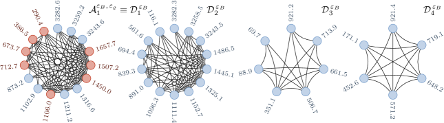
Figure 1: Partitioning of $S_{1}$ normal-mode coordinates of dithiophene T$2$ into approximately independent subsets for the threshold value $\varepsilon_{B}=0.045$ [see Eq. (22)]. Colored circles represent individual modes, i.e., elements of $\mathcal{D}$. The dynamically important modes [Eq. (25)] comprising $\mathcal{G}^{\varepsilon_{\varrho}}$ with the threshold value $\varepsilon_{\varrho}=0.6$ are shown in red. Finally, solid lines represent inter-mode couplings above the threshold $\varepsilon_{B}$. Vibrational frequencies are given in cm^-1.

III Computational details

All ab initio calculations were performed with the Gaussian09 package.Frisch et al. Its output was extracted directly from the checkpoint file. The ground PES $S_{0}$ was handled with the density functional theory (DFT), whereas the first excited singlet PES ($S_{1}$) was described with the time-dependent DFT (TD-DFT). Following the work of Stendardo et al., our TD-DFT calculations were based on the long-range corrected CAM-B3LYP functionalStendardo et al. (2012) with 6-31+G(d,p) basis set. Within this TD-DFT setup, the energy gap between the $S_{0}$ and $S_{1}$ PESs of oligothiophenes is described quite accurately. Although Gaussian09 provides analytical gradients for both DFT and TD-DFT, analytical Hessians are available only for DFT. No symmetry constraints were enforced and the ‘‘fine’’ and ‘‘ultra fine’’ integration grids were used for OTF-AI calculations and geometry optimization, respectively.

In order to find the physically relevant equilibrium geometry of $S_{1}$ for each oligothiophene T$n$, we first performed an $S_{0}$ geometry optimization of the ‘‘all-trans’’ conformer, the rings of which are oriented in an anti conformation with respect to their neighbors. The work by Becker and co-workersBecker et al. (1996) suggests that this is the most stable conformer. The $S_{1}$ geometry optimization was started from this $S_{0}$ equilibrium geometry. It has been well-established that in contrast to the inter-ring twisted $S_{0}$ equilibrium geometry and its shallow potential, $S_{1}$ exhibits a steep, deep, harmonic-like well in the vicinity of its planar equilibrium geometry.Belletete, Leclerc, and Durocher (1994); Becker et al. (1996) The $S_{1}$ equilibrium geometry, shown in the Supplementary Material,sup served as the reference structure for the OTF-AI-TGA dynamics.

Within the OTF-AI-TGA, the GWP was propagated for the total time of $7976\,\text{a.u.}\approx 193\,\text{fs}$ with a time step of $8\,\text{a.u.}\approx 0.2\,\text{fs}$ using the second order symplectic algorithm. The resulting spectra were subjected to a phenomenological (inhomogeneous) Gaussian broadening with half-width at half-maximum (HWHM) of $0.025$$\,\text{eV}\approx 200\,\text{cm}^{-1}$.

IV Results and discussion

IV.1 Comparison with experimental spectra

Our results confirm the utility of the OTF-AI-TGA approach for electronic spectra calculation, since all important features of the experimental spectra are almost perfectly reproduced. Figure 2 demonstrates the agreement with the overall shape, peak intensities, as well as the trend of the spectra to gradually shift towards lower frequencies with increasing number of rings in the molecule. Note that particular experimental conditions, notably the interaction with the solvent (here, ethanol glass at $77\,$K), can produce a shift of the spectrum. However, we disregard this effect since the resulting shift is expected to be small for a broad class of solvents.Becker et al. (1996); Belletete, Leclerc, and Durocher (1994); Chadwick and Kohler (1994) Also, the exact prediction of the spectrum position is partly beyond the level of the ab initio setup employed here (see Sec. III).

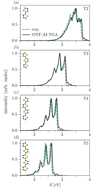
Figure 2: Emission spectra of the oligothiophene T$n$ family for $n\in\{2,3,4,5\}$: Comparison of experimental emission spectra (exp., dashed green line) with the full-dimensional OTF-AI-TGA calculations using all 21$n$ normal modes (solid black line).

Becker et al.Becker et al. (1995) reported a significant red shift of the oligothiophene absorption spectra at low temperatures and attributed this phenomenon to the twisted$\mapsto$planar conformational transition induced by solvent freezing. Interestingly, this shift was not observed in the emission spectra, which suggests that in the whole temperature range it is only the planar conformation that plays a significant role in this process. Even without imposing explicit planarity constraints, no deviations from the planar conformation were observed during the ground-state gas-phase OTF-AI dynamics due to planarity of the initial geometry. This fact makes the comparison of our gas-phase results to the experimental data more legitimate. Finally note that the ab initio ground state equilibrium geometry is twisted in contrast to the equilibrium geometry in ethanol glass at $77\,$K. Therefore, the $n-1$ torsional degrees of freedom connecting the planar and twisted geometries of T$n$ have imaginary frequencies. Since our approach is unable to describe wave-packet splitting, the TGA GWP only spreads along these degrees of freedom (see Supplementary Material,sup Sec. E). However, since we are mainly interested in short-time dynamics, this behavior is qualitatively correct. Hence, the OTF-AI-TGA approach remains in this case robust even for floppy molecules and the question about the ‘‘harmonicity’’ of the system is of much lesser importance due to the employment of the local harmonic approximation. Although the global harmonic approximation is quite adequate for T$n$,Stendardo et al. (2012) small changes of the peak positions and intensities can be observed as compared to OTF-AI-TGA (see Supplementary Material,sup Sec. F).

To facilitate comparison between line-shape spectra of oligothiophenes with different numbers of thiophene rings, the spectra shown in Fig. 3(a) are first $L^{\infty}$ normalized and subsequently shifted so that the ‘‘$\alpha_{0}$-peaks’’ overlap at zero energy. This reveals that the relative peak positions are rather insensitive to $n$, while their prominence is increasing with increasing $n$. The peak at the highest energy (in our notation: $\alpha_{0}$) in the emission spectrum is attributed to the $0$–$0$ transition.Gierschner, Cornil, and Egelhaaf (2007) The position of the $\alpha_{1}$-peak is close to the vertical transition energy $E_{\text{vert}}$, which, in loose terms, justifies its dominance in Fig. 3(a). More detailed classification of individual spectral peaks into the $\alpha,\beta$ groups and their interpretation from the dynamical viewpoint is discussed in Subsec. IV.2.

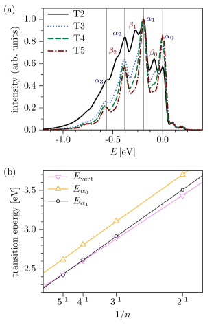
Figure 3: Emission in the oligothiophene T$n$ family for $n\in\{2,3,4,5\}$. (a) $L^{\infty}$-normalized line-shape spectra. To facilitate their comparison, the spectra are shifted independently for each $n$ so that the $\alpha_{0}$ peak appears at zero energy. (b) Dependence of the vertical-transition energy $E_{\text{vert}}$ and positions of the $\alpha_{0}$ and $\alpha_{1}\text{-peaks}$ $(E_{\alpha_{0}},\,E_{\alpha_{1}})$ on $1/n$ (see text for details). Linear fits are denoted with lines.

It has been found experimentally that the $0$–$0$ transition energy $E_{0\text{--}0}$ in the polythiophene family T$n$ is a linear function of $1/n$.Becker et al. (1996); Yang et al. (1997, 1998); Thémans, Salaneck, and Brédas (1989) In accordance with this observation and our identification of $E_{0\text{--}0}$ with $E_{\alpha_{0}}$, we found that $E_{\alpha_{0}}$ is accurately described by the function $E_{\alpha_{0}}(n)\approx(3.58/n+1.91)\,\text{eV}$. Good agreement with the experiment can be directly inferred from Fig. 2. Furthermore, from the ab initio data, we determined in a similar fashion that $E_{\text{vert}}(n)\approx(3.33/n+1.77)\,\text{eV}$. Fits of $E_{\alpha_{0}}$, $E_{\alpha_{1}}$ and $E_{\text{vert}}$ are shown in Fig. 3(b).

Note that the relative intensity of the $\alpha_{0}$-peak, identified with the $0$–$0$ transition, in Fig. 3(a) increases with $n$. This can be related to the fact that the slope of $E_{\alpha_{1}}(n)$ is larger than the slope of $E_{\text{vert}}(n)$ [see Fig. 3(b)], using the following heuristic argument: Neglecting the difference between the $S_{0}$ and $S_{1}$ zero-point energies, the $0$–$0$ transition energy depends solely on the energy gap between these PESs. On the other hand, $E_{\text{vert}}$ is influenced also by the relative displacement of the $S_{0}$ and $S_{1}$ potential minima. Therefore, if $E_{\text{vert}}$ decreases more slowly with increasing $n$ than does the $0$–$0$ transition energy, one can expect a decrease not only in the energy gap between $S_{0}$ and $S_{1}$ PESs but also in the relative displacement of their minima, which, in turn, is responsible for the gain in intensity of the $0$–$0$ transition, i.e., the $\alpha_{0}$-peak. This observation is in agreement with the Huang-Rhys analysis performed by A. Yang et al.Yang et al. (1998) on fluorescence spectra of T$n$ for $n\in\{3,4,5,6\}$.

IV.2 Vibrational analysis

To gain a deeper understanding of the emission spectra shown in Figs. 2 and 3, we employ independently for each oligothiophene T$n$ the analysis proposed in Subsec. II.5 adapted to the normal-mode coordinates of the $S_{1}$ PES of T$n$. To this end, we closely follow the example presented at the end of Subsec. II.5. The normal-mode classification based on decompositions (27) and (29) with $\varepsilon_{B}=0.55$ and $\varepsilon_{\rho}=0.6$ results for all T$n$ in an active space $\mathcal{A}$ comprised of six groups of modes (see Tab. 1). This space is spanned by ten ‘‘active’’ modes (i.e., $\lvert\mathcal{A}\rvert=10$) for T$2$-T$4$, while $\lvert\mathcal{A}\rvert=8$ for T$5$. The thresholds were chosen in order to obtain a minimal set $\mathcal{A}$ of active modes with as many subsets as possible on condition that the reduced OTF-AI-TGA spectrum $\sigma_{\mathcal{A}}$ recovers all important features of the ‘‘complete’’ spectrum $\sigma_{\mathcal{D}}$. For clarity, the subscript of $\sigma$ denotes explicitly the set of modes taken into account in the spectra calculation. Formally, the spectrum $\sigma_{\mathcal{A}}$ can be thought of as the computationally cheapest, yet still sufficiently accurate approximation of $\sigma_{\mathcal{D}}$.

For details regarding correlation function and spectra calculations within proper subspaces of $\mathcal{D}$ we refer to the Appendix A. From now on, to simplify notation, the implicit dependence of, e.g., $\mathcal{A}$ on the threshold values $\varepsilon_{B}$ and $\varepsilon_{\varrho}$ will not be denoted explicitly.

Figure 4(a) demonstrates that ten modes were sufficient to essentially reproduce the complete spectrum $\sigma_{\mathcal{D}}$ for T$2$. The simplification achieved is the most striking for T$5$ [Fig. 4(b)], for which eight modes were sufficient and hence the dimensionality was reduced more than ten times without losing any major feature in the spectrum. However, note that the ‘‘$\lvert\mathcal{A}\rvert$-mode’’ spectra in Fig. 4 are slightly shifted due to dependence of the zero-point energy on the choice of $\mathcal{A}$. (Analogous spectra of T$3$ and T$4$ are shown in Sec. B of the Supplementary Material.sup )

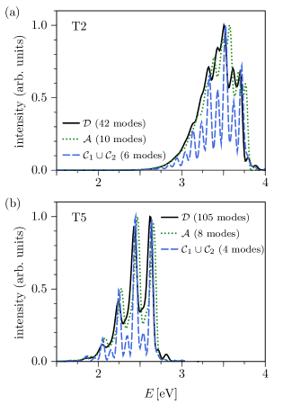
Figure 4: Emission spectra of oligothiophenes T$2\,$(a) and T$5\,$(b): comparison of the full-dimensional OTF-AI-TGA spectrum $\sigma_{\mathcal{D}}$ (solid black line) with the spectrum $\sigma_{\mathcal{A}}$ (dotted green line) computed within the subspace $\mathcal{A}$ of the active modes and the spectrum $\sigma_{\mathcal{C}_{1}\cup\,\mathcal{C}_{2}}$ (dashed blue line) taking into account only modes belonging to the classes $\mathcal{C}_{1}$ and $\mathcal{C}_{2}$ (see Fig. 6 and Tab. 1) introduced in Eq. (29).

The modes in $\mathcal{A}$ are by definition considered to be coupled only within individual groups. Therefore, one can attempt to assign a characteristic vibrational movement of the entire molecule induced by excitation of the modes belonging to a particular group. Among the $24$ groups ($24=4$ oligothiophenes $\times$ $6$ groups per oligothiophene), we identified $7$ characteristic motions shown on the examples of T$3$ and T$4$ molecules in Fig. 5. In Table 1, these characteristic motions are distinguished with a superscript.

(a) inter-ring stretch	(b) ring squeeze	(c) chain deformation
(d) inner-ring C-S-C stretch	(e) ring expansion	(f) C-H deformation
(g) C-S-C outer-ring asymmetric stretch

Figure 5: Characterization of the active normal modes in the set $\mathcal{A}\subseteq\mathcal{D}$ [see Eqs. (27) and (29)] by the nature of the deformation which they exert on the oligothiophene T$n$ skeleton. To cover all cases presented in Tab. 1, these deformations are shown on the examples of T$3$ and T$4$ . Panel labels correspond to the classification in Tab. 1.

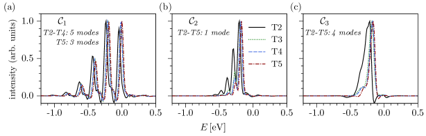
Figure 6: Classification of normal modes of the oligothiophene T$n$ family according to their influence on the resulting emission spectrum [see Eqs. (27) and (29)]. Detailed description of individual classes is contained in Tab. 1. (a) Inter-ring stretch modes responsible for the $\alpha$-peaks shown in Fig. 3. (b) Ring-squeeze mode reflected in the $\beta$-peaks in Fig. 3. (c) Remaining modes causing overall broadening of the spectra.

Next, the six groups of normal modes are, for each $n\in\{2,3,4,5\}$, merged into three disjoint classes $\mathcal{C}_{1}$, $\mathcal{C}_{2}$, and $\mathcal{C}_{3}$ as

$$\mathcal{C}_{1}:=\mathcal{A}_{1},\text{ }\mathcal{C}_{2}:=\mathcal{A}_{2},\text{ and }\mathcal{C}_{3}:=\bigcup_{\alpha=3}^{6}\mathcal{A}_{\alpha}.$$ (29)

The reason for introducing an additional logical layer is the observation in Fig. 6 that the overall character of the spectrum $\sigma_{\mathcal{C}_{i}}$ corresponding to the $i$th group is only mildly influenced by $n$, whereas the dependence on $i$ is dominant. In loose terms, the first group $\mathcal{C}_{1}$ comprises inter-ring stretch modes and is mainly reflected in the ‘‘$\alpha$-peaks’’ of the complete spectrum $\sigma_{\mathcal{D}}$ [see Fig. 3(a)]. The second group $\mathcal{C}_{2}$ consists of a ring-squeeze mode and produces the ‘‘$\beta$-peaks’’ in Fig. 3(a). Finally, the modes contained in the third group cause merely an overall broadening of the spectrum. Such a classification of vibrational modes, essential for a theoretical interpretation of the emission spectra, is also useful in practice, e.g., in the design of organic light-emitting diodes (OLEDs).Lumpi et al. (2013)

The difference between individual classes is further emphasized by introducing an ‘‘overall relative displacement’’ of the $i$th class as $R_{i}^{2}:=\sum_{j\in\mathcal{C}_{i}}\varrho_{j}^{2}$. We have found that $R_{1}$ is highly correlated with $-n$ while $R_{2}$ with $1/n$. Therefore, for low $n$, the dynamical importance of the class $\mathcal{C}_{2}$ decreases faster with increasing $n$. This results in less structured spectra, shown in Fig. 3(b), in which the $\beta$-peaks are almost invisible already for T$3$.

In summary, the inter-ring stretch motion is seen to have a dominant effect on the T$n$ spectra, especially for $n>2$. Comparing the relative displacements of the classes $\mathcal{C}_{1}$ and $\mathcal{C}_{2}$ helps to further corroborate the hypothesis (stated above) that the $S_{0}$ and $S_{1}$ geometries become less displaced with increasing $n$ since the $0$–$0$ transition energy $E_{0\text{--}0}(n)$ decreases faster than the vertical excitation energy $E_{\text{vert}}(n)$.

IV.3 Quinoid structure of $S_{1}$

The extent of $\pi$-conjugation along the oligomer chain is reflected in the quinoid structure of individual rings. The degree of the quinoid/aromatic character of the $i$th ring in T$n$ can be quantified in terms of the so-called bond length alternationBeljonne et al. (1996); Fazzi et al. (2010); Ponce Ortiz et al. (2010) (BLA)

$$\text{BLA}_{i}=R_{\beta_{i}}-(R_{\alpha_{i}}+R_{\alpha_{i}^{\prime}})/2,$$ (30)

where $R$ denotes the length of the $\beta$, $\alpha$, and $\alpha^{\prime}$ bonds of the $i$th ring (see Fig. 7). Hence, quinoid rings have a negative BLA, while aromatic rings have a positive BLA.

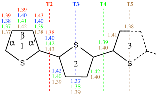
Figure 7: Equilibrium $S_{1}$ geometry of oligothiophenes T$n$ for $n\in\{2,3,4,5\}$. Corresponding bond lengths for different oligothiophenes T$n$ are juxtaposed with each other next to individual bonds, whereas the dashed lines represent the end of the half-chain for each T$n$. E.g., to the right of the dashed line marked as T$3$ there are only one or two bond-length values since those bonds are not present in the half-chain of T$2$ and T$3$.

The $S_{1}$ equilibrium geometries of T$n$ in Fig. 7 reveal that for $n>2$, both quinoid and aromatic ring types are present in the chain: The inner rings are quinoid, while the end rings are aromatic. On the other hand, both rings of T$2$ have quinoid character. However, the large difference between the lengths of $\alpha$ and $\alpha^{\prime}$ bonds suggests a double-bond character of the outer $\alpha$ bond in T₂. In general, the DFT $S_{1}$ geometries exhibit more pronounced quinoid character in comparison with the $S_{1}$ geometries calculated at the MNDO level,Beljonne et al. (1996) which describe T$2$ as slightly aromatic.

The time dependence of BLA, displayed for T$5$ in Fig. 8 and for T2, T3, and T4 in Sec. C of the Supplementary Material,sup shows emission-induced oscillations between the quinoid and aromatic characters of individual rings. The inner rings are seen to be subjected to larger structural variations, while the outer rings remain aromatic, although the degree of aromaticity changes periodically. Hence, the quinoid character of T$n$ in $S_{1}$ is well localized over just $2$-$3$ rings, as was shown also by Beljonne et al.,Beljonne et al. (1996) while the emission process triggers deformation of the whole chain.

Oligomer vibrational line shapes are usually analyzed in terms of the effective conjugation coordinateZerbi et al. (1989); Geisselbrecht, Kürti, and Kuzmany (1993); Zerbi, Castiglioni, and Del Zoppo (2007) (ECC)—a totally symmetric internal coordinate describing the variation of adjacent C-C backbone stretches, responsible for the change from the aromatic to quinoid structure. A detailed analysis (summarized in Appendix B) of the dynamics shows that only some of the modes coupled to ECC are also excited by the fluorescence process. The overall contribution of the $\mathcal{A}_{1}$ group to the ECC is more than $92$% for all olighothiophenes and, hence, the $\alpha$-peaks originate from the change of the ECC during the dynamics induced by the fluorescence process.

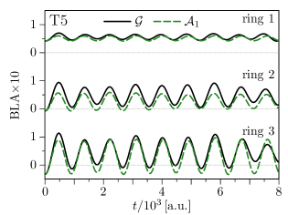
Figure 8: Time dependence of the bond length alternation (BLA) parameter during the dynamics induced by the emission in pentathiophene T$5$ [see Eq. (30) and Fig. 7]. The character of the outer rings (rings $1$ and $2$) is mainly aromatic (positive BLA), while the transition to the quinoid structure (negative BLA) occurs almost exclusively within the inner ring (ring $3$).

Table 1: Normal-mode classification based on decompositions (27) and (29) with $\varepsilon_{B}=0.55$ and $\varepsilon_{\rho}=0.6$ for the oligothiophene T$n$ family, $n\in\{2,3,4,5\}$. Vibrational frequencies $\omega_{i}$ are given in cm^-1, while the maximum relative displacements $\rho_{i}$ of Eq. (24) are dimensionless. The modes are further classified into $7$ groups by the character of the deformation which they exert on the oligothiophene skeleton. These groups are distinguished by superscript labels next to frequency values. For schematic depiction of these deformations see Fig. 5.

class	group	$\omega_{i}\,$[cm-1]				$\rho_{i}$
		T$2$	T$3$	T$4$	T$5$	T$2$	T$3$	T$4$	T$5$
$\mathcal{C}_{1}$	$\mathcal{A}_{1}$	$1657.7\mbox{${}^{\scriptscriptstyle(a)}$}$	$1630.5\mbox{${}^{\scriptscriptstyle(a)}$}$	$1615.5\mbox{${}^{\scriptscriptstyle(a)}$}$	$1598.6\mbox{${}^{\scriptscriptstyle(a)}$}$	$2.57\mbox{${}^{\scriptscriptstyle(a)}$}$	$2.50\mbox{${}^{\scriptscriptstyle(a)}$}$	$2.41\mbox{${}^{\scriptscriptstyle(a)}$}$	$1.93\mbox{${}^{\scriptscriptstyle(a)}$}$
		$1507.2\mbox{${}^{\scriptscriptstyle(a)}$}$	$1553.9\mbox{${}^{\scriptscriptstyle(a)}$}$	$1545.2\mbox{${}^{\scriptscriptstyle(a)}$}$	$1590.1\mbox{${}^{\scriptscriptstyle(a)}$}$	$1.23\mbox{${}^{\scriptscriptstyle(a)}$}$	$1.10\mbox{${}^{\scriptscriptstyle(a)}$}$	$1.12\mbox{${}^{\scriptscriptstyle(a)}$}$	$1.35\mbox{${}^{\scriptscriptstyle(a)}$}$
		$1450.0\mbox{${}^{\scriptscriptstyle(a)}$}$	$1501.2\mbox{${}^{\scriptscriptstyle(a)}$}$	$1581.3\mbox{${}^{\scriptscriptstyle(a)}$}$	$1548.5\mbox{${}^{\scriptscriptstyle(a)}$}$	$0.88\mbox{${}^{\scriptscriptstyle(a)}$}$	$0.86\mbox{${}^{\scriptscriptstyle(a)}$}$	$0.56\mbox{${}^{\scriptscriptstyle(a)}$}$	$1.13\mbox{${}^{\scriptscriptstyle(a)}$}$
		$1211.2\mbox{${}^{\scriptscriptstyle(a)}$}$	$1461.9\mbox{${}^{\scriptscriptstyle(a)}$}$	$1498.2\mbox{${}^{\scriptscriptstyle(a)}$}$		$0.59\mbox{${}^{\scriptscriptstyle(a)}$}$	$0.36\mbox{${}^{\scriptscriptstyle(a)}$}$	$0.55\mbox{${}^{\scriptscriptstyle(a)}$}$
		$3243.6\mbox{${}^{\scriptscriptstyle(a)}$}$	$1341.6\mbox{${}^{\scriptscriptstyle(a)}$}$	$1462.6\mbox{${}^{\scriptscriptstyle(a)}$}$		$0.25\mbox{${}^{\scriptscriptstyle(a)}$}$	$0.34\mbox{${}^{\scriptscriptstyle(a)}$}$	$0.36\mbox{${}^{\scriptscriptstyle(a)}$}$
$\mathcal{C}_{2}$	$\mathcal{A}_{2}$	$673.7\mbox{${}^{\scriptscriptstyle(b)}$}$	$696.7\mbox{${}^{\scriptscriptstyle(b)}$}$	$704.7\mbox{${}^{\scriptscriptstyle(b)}$}$	$710.8\mbox{${}^{\scriptscriptstyle(b)}$}$	$2.05\mbox{${}^{\scriptscriptstyle(b)}$}$	$1.56\mbox{${}^{\scriptscriptstyle(b)}$}$	$1.32\mbox{${}^{\scriptscriptstyle(b)}$}$	$1.17\mbox{${}^{\scriptscriptstyle(b)}$}$
$\mathcal{C}_{3}$	$\mathcal{A}_{3}$	$290.4\mbox{${}^{\scriptscriptstyle(e)}$}$	$210.1\mbox{${}^{\scriptscriptstyle(e)}$}$	$162.3\mbox{${}^{\scriptscriptstyle(e)}$}$	$122.5\mbox{${}^{\scriptscriptstyle(c)}$}$	$1.27\mbox{${}^{\scriptscriptstyle(e)}$}$	$1.92\mbox{${}^{\scriptscriptstyle(e)}$}$	$2.15\mbox{${}^{\scriptscriptstyle(e)}$}$	$0.99\mbox{${}^{\scriptscriptstyle(c)}$}$
	$\mathcal{A}_{4}$	$386.5\mbox{${}^{\scriptscriptstyle(c)}$}$	$350.3\mbox{${}^{\scriptscriptstyle(c)}$}$	$333.0\mbox{${}^{\scriptscriptstyle(c)}$}$	$136.7\mbox{${}^{\scriptscriptstyle(c)}$}$	$1.61\mbox{${}^{\scriptscriptstyle(c)}$}$	$1.49\mbox{${}^{\scriptscriptstyle(c)}$}$	$1.39\mbox{${}^{\scriptscriptstyle(c)}$}$	$2.09\mbox{${}^{\scriptscriptstyle(c)}$}$
	$\mathcal{A}_{5}$	$712.7\mbox{${}^{\scriptscriptstyle(g)}$}$	$739.6\mbox{${}^{\scriptscriptstyle(g)}$}$	$1112.9\mbox{${}^{\scriptscriptstyle(f)}$}$	$322.6\mbox{${}^{\scriptscriptstyle(c)}$}$	$1.09\mbox{${}^{\scriptscriptstyle(g)}$}$	$0.64\mbox{${}^{\scriptscriptstyle(g)}$}$	$0.63\mbox{${}^{\scriptscriptstyle(f)}$}$	$1.35\mbox{${}^{\scriptscriptstyle(c)}$}$
	$\mathcal{A}_{6}$	$1096.3\mbox{${}^{\scriptscriptstyle(f)}$}$	$1261.6\mbox{${}^{\scriptscriptstyle(d)}$}$	$1275.0\mbox{${}^{\scriptscriptstyle(d)}$}$	$1109.5\mbox{${}^{\scriptscriptstyle(f)}$}$	$0.78\mbox{${}^{\scriptscriptstyle(f)}$}$	$0.70\mbox{${}^{\scriptscriptstyle(d)}$}$	$0.66\mbox{${}^{\scriptscriptstyle(d)}$}$	$0.78\mbox{${}^{\scriptscriptstyle(f)}$}$

V Conclusion

All features of the experimental emission spectra of oligothiophenes with up to five rings (i.e., up to $105$ vibrational DOFs) are well reproduced by our OTF-AI-TGA calculations. The efficiency of the TGA formulation is found to allow treating all vibrational DOFs on an equal footing even in case of larger systems especially since the OTF-AI scheme does not require an a priori knowledge of the potential energy surfaces and the TGA approach remains robust for floppy molecules. No symmetry considerations are necessary; in particular, neither the dynamics nor the analysis relies on any symmetry assumptions. Moreover, further considerable gain in efficiency without loosing any substantial information can be obtained by employing Hessian interpolation.

Experimentalists try, often successfully, to translate the spectral features into a dynamical picture, which for theoreticians is often the starting point. The extraction of the essential information from the dynamical simulation, however, is often as difficult as the simulation itself. We presented, therefore, a novel systematic approach to identify groups of vibrations that are essential for the dynamics and for the spectrum. This approach even allowed us to compare different oligothiophenes T$n$ and to study changes in their spectra with increasing $n$: Their vibrational line shapes are modulated by inter-ring stretch and ring-squeeze vibrations, the latter contributing to the spectral broadening for longer chains. The ground and excited potential energy surfaces become more similar as the chain length increases; this, in turn, reduces the amplitude of the dynamics induced by emission and results in a shift of the intensity toward the $0$–$0$ transition. The phenomenon is also reflected in the different dependences of the $0$–$0$ and vertical transition energies on $1/n$.

The OTF-AI-TGA scheme also allowed us, by evaluating the bond length alternation, to study directly dynamical oscillations between the quinoid and aromatic characters of individual rings in the oligothiophene chain.

OTF-AI-TGA is also useful as a preliminary test. The expensive OTF-AI information stored during the TGA simulation can be reused in other semiclassical methods such as poor person’s Herman-Kluk (HK) propagator, where the HK prefactor is for all contributing trajectories assumed to be equal to the prefactor of the central trajectory.Tatchen et al. (2011) In systems, which are too large to be treated with a more sophisticated quantum or semiclassical method, but for which the TGA is insufficient, e.g., due to the importance of interference effects, the analysis of the OTF-AI-TGA results can be used to define a subspace of reduced dimensionality, in which the most important dynamics occurs. Within this subspace, the effects that cannot be described with the TGA may be studied with less efficient yet better-suited methods.Grossmann (2006) Alternative approaches for constructing the information-flow matrix in order to maximize the decoupling of the DOFs with minimal impact on the resulting spectrum are the subject of our ongoing research.

Finally, let us note that the computational protocol presented here is not limited to linear spectroscopy; non-linear spectra such as time-resolved stimulated emission can also be evaluated with the OTF-AI-TGA.

Appendix A TGA in subspaces of reduced dimensionality

One of the main goals of the normal mode analysis elaborated in Subsec. II.5 is identifying the normal modes essential for the dynamics. Restriction to these most important modes allows one to devise a simplified model of reduced dimensionality, e.g., in the spirit of the well-studied pyrazine vibronic coupling model.Stock et al. (1995) Moreover, this reduction also broadens the class of computationally available methods. After the reduction, one may be able to employ, e.g., the Gaussian basis methods,Shalashilin and Child (2000); *Worth_Burghardt:2004; *Martinez_ACP_02 or various approaches from the family of the semiclassical initial value representation.Miller (2001); *Herman:1994; *Thoss_Wang:2004; *Kay:2005

Let us consider a system with $D$ vibrational DOFs. In a typical OTF-AI-TGA calculation, one evolves the $D$-dimensional GWP by classically propagating its center $x^{t}$ and by evaluating the phase factor $\gamma^{t}$ and the complex time-dependent width matrix $A^{t}$ by means of Lee and Heller’s $P$-$Z$ algorithmLee and Heller (1982) summarized in Subsec. II.2 [Eqs. (11) and (8)].

As in Subsec. II.5, we identify the $D$-dimensional space of vibrational DOFs with the set $\mathcal{D}=\{1,\ldots,D\}$. We would like to take advantage of the stored $D$-dimensional trajectory information, and, at the same time, to restrict ourselves to a subset $\mathcal{P}\subseteq\mathcal{D}$ of only $d<D$ most important vibrational degrees of freedom and define a linear projection $\pi\!:\,\mathbb{R}^{D}\rightarrow\mathbb{R}^{d}$ from the full space of $D$ vibrational DOFs to the subspace of physical interest. Formally

$$\pi_{ij}:=\delta_{\mathcal{P}_{i},j}\text{ for }1\leq{}i\leq{}d\text{ and }1\leq j\leq D,$$ (31)

where $\mathcal{P}_{i}$ denotes the $i$th element of the ordered set $\mathcal{P}$.

The ‘‘reduced’’ $d$-dimensional GWP is again propagated using the $P$-$Z$ formalism. However, if $(q^{t},\,p^{t})$ denotes the trajectory followed by the original, $D$-dimensional GWP, then the center of the reduced Gaussian follows a classical trajectory $\left(\pi\cdot q^{t},\pi\cdot p^{t}\right)$ in the reduced, $2d$-dimensional phase space. Also, the initial conditions for the time-dependent $P^{t},\,Z^{t}$ matrices must be replaced with

$$\bar{Z}^{0} =\pi\cdot\pi^{\mathsf{T}}=I_{d},$$ (32a)

$$\bar{P}^{0} =2i\hbar\,\pi\cdot A^{0}\cdot\pi^{\mathsf{T}}.$$ (32b)

Here, $$d A^{0} D$$-dimensional matrices are denoted with a bar and is the initial width matrix of the -dimensional GWP.

Finally, we need to isolate the $\mathcal{P}$-contribution to the effective Lagrangian $\mathcal{L}_{\text{eff}}$, which is required in Eq. (11) for evaluating the time-dependent complex phase $\gamma^{t}$. This is conveniently done using conservation of energy, since in all our calculations we consider only stationary initial states. Therefore

$$\frac{1}{2}{\zeta^{t}}^{\mathsf{T}}\cdot\zeta^{t}+V(\eta^{t})=V(\eta^{0}),$$ (33)

with $\zeta$ denoting momentum conjugated to $\eta$; mass factors do not explicitly appear since $\eta$ is already mass-scaled. Using Eq. (33), the $\mathcal{L}_{\text{eff}}$-contribution to $\gamma^{t}$ in Eq. (11) then reads

$$\int_{0}^{t}\mathcal{L}_{\text{eff}}^{\tau}\,d\tau =\int_{0}^{t}\!\bigl{[}\frac{1}{2}({\zeta^{\tau}})^{\mathsf{T}}\cdot\zeta^{\tau}-V(\eta^{\tau})\bigr{]}d\tau$$

$$=\int_{0}^{t}\!\bigl{[}({\zeta^{\tau}})^{\mathsf{T}}\cdot\zeta^{\tau}-V(\eta^{0})\bigr{]}d\tau$$

$$=\int_{0}^{t}\!({\zeta^{\tau}})^{\mathsf{T}}\cdot\zeta^{\tau}\,d\tau-V(\eta^{0})\,t.$$ (34)

The part of this expression pertinent to the dynamics within the subset of vibrational DOFs $\mathcal{P}$ is then easily obtained by replacing $\zeta^{t}$ with $\pi\cdot\zeta^{t}$, i.e.,

$$\left.\int_{0}^{t}\mathcal{L}_{\text{eff}}^{\tau}\,d\tau\right|_{\mathcal{P}}=\int_{0}^{t}\!(\pi\cdot{\zeta^{\tau}})^{\mathsf{T}}\cdot(\pi\cdot\zeta^{\tau})\,d\tau-V(\eta^{0})\,t.$$ (35)

The term $V(\eta^{0})\,t$ generates an overall phase depending linearly on $t$ and is responsible only for shift of the resulting spectrum without altering its shape.

Appendix B Analysis of the effective conjugation coordinate

Oligomer spectra are usually analyzed in terms of the so-called effective conjugation coordinateZerbi et al. (1989); Geisselbrecht, Kürti, and Kuzmany (1993); Zerbi, Castiglioni, and Del Zoppo (2007) (ECC), i.e., the totally symmetric internal coordinate the excitation of which triggers the conformational change between the aromatic to the quinoid structures of the molecule. This approach is especially popular within Raman spectroscopy.Lopez Navarrete and Zerbi (1991); Zerbi, Chierichetti, and Ingänas (1991); Castiglioni, Tommasini, and Zerbi (2004); Ortí et al. (2005); Fazzi et al. (2010) For the oligothiophene family T$n$, ECC captures the alternation between adjacent bonds and is defined as

$$\mbox{Я}:=\frac{1}{\sqrt{\bar{N}}}\sum_{a=1}^{\bar{N}}(-1)^{a-1}r_{a},$$ (36)

where $r_{a}$ is the Cartesian vector connecting the $a$th and $(a+1)$th carbon atoms of the backbone comprised of $\bar{N}=4n-1$ C-C bonds in total. Further insight is gained by restating Eq. (36) in the normal-mode coordinates. By employing transformation (12), we obtain

$$\mbox{Я}=\mbox{Я}_{\text{ref}}+\mathrm{R}\cdot\eta\text{, with }\mathrm{R}:=\mathrm{S}\cdot T\text{ and }\mbox{Я}_{\text{ref}}:=\mathrm{S}\cdot\xi_{\text{ref}},$$ (37)

where $T$ is the transformation matrix of Eq. (12), $\xi_{\text{ref}}$ denotes Cartesian coordinates of a reference geometry, and

$$\mathrm{S}:=\frac{1}{\sqrt{\bar{N}}}\sum_{a=1}^{\bar{N}}(-1)^{a}(\mathrm{P}_{a}-\mathrm{P}_{a+1})$$ (38)

is a generalization of the projector $\mathrm{P}_{b}$ defined below Eq. (13).

Then, the normalized “coupling strength” $\nu^{j}$ of the $j$th normal mode to Я reads

$$\nu^{j}:=\frac{\mathop{\mathrm{Tr}}\mathrm{Y}_{j}^{\mathsf{T}}\!\cdot\mathrm{R}^{\mathsf{T}}\!\cdot\mathrm{R}\cdot\mathrm{Y}_{j}}{\mathop{\mathrm{Tr}}\mathrm{R}^{\mathsf{T}}\!\cdot\mathrm{R}},$$ (39)

where the square matrix $\mathrm{Y}_{j}$ is defined as $(\mathrm{Y}_{j})_{kl}:=\delta_{jk}\delta_{jl}$.

However, the quantity Я changes during the dynamics and its variations are described in terms of

$$\delta\mbox{Я}^{t}:=\mbox{Я}^{t}-\mbox{Я}^{0}=\mathrm{R}\cdot{\bar{\eta}^{t}}\text{, with }\bar{\eta}^{t}:=(\eta^{t}-\eta^{0}).$$ (40)

Now, in order to asses the importance of a particular normal mode with respect to $\delta\mbox{Я}^{t}$, we can not use Eq. (39) directly, since $\nu^{j}$ provides only a static picture. To remedy this, we introduce a more appropriate measure of dynamical coupling:

$$\upsilon^{j}:=\frac{\varsigma^{j}}{\sum_{k}\varsigma^{k}}\text{, with }\varsigma^{j}:=\int_{0}^{t}\!dt\,\bar{\eta}^{t}\cdot\mathrm{Y}_{j}^{\mathsf{T}}\!\cdot\mathrm{R}^{\mathsf{T}}\!\cdot\mathrm{R}\cdot\mathrm{Y}_{j}\cdot\bar{\eta}^{t},$$ (41)

where the summation runs over all normal modes.

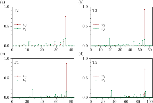
Figure 9: Comparison of the static, $\nu_{j}$ [see Eq. (39)], and dynamic, $\upsilon_{j}$ [see Eq. (41)], contribution of individual normal modes to the ECC Я of Eq. (36) for the oligothiophenes T$n$, $n\in\{2,3,4,5\}$.

A comparison of individual normal modes for T$n$, $n\in\{2,3,4,5\}$, in terms of $\nu^{j}$ and $\upsilon^{j}$ is shown in Fig. 9, which demonstrates clearly that only certain modes contributing to Я are excited during the fluorescence process. This means that an analysis based merely on $\nu^{j}$ would be incomplete.

In Subsec. II.5, individual normal modes were classified into independent groups $\mathcal{A}_{i}$ [see Eq. (27)]. Using Eq. (41), we can estimate the dynamical influence of a particular group $\mathcal{A}_{i}$ on $\delta\mbox{Я}^{t}$ by employing

$$\kappa_{i}:=\sum_{j\in\mathcal{A}_{i}}\upsilon^{j}.$$ (42)

Table 2 demonstrates that variations in Я can be assigned mostly to the group $\mathcal{A}_{1}$, and, hence, the $\alpha$-peaks (see Fig. 3) originate from the change of the ECC during the dynamics induced by the fluorescence process.

	$\mathcal{A}_{1}$	$\mathcal{A}_{2}$	$\mathcal{A}_{3}$	$\mathcal{A}_{4}$	$\mathcal{A}_{5}$	$\mathcal{A}_{6}$
T$2$	0.947	0.013	0.006	0.006	0.008	0.015
T$3$	0.962	0.010	0.009	0.001	0.000	0.003
T$4$	0.942	0.009	0.010	0.002	0.004	0.013
T$5$	0.927	0.008	0.000	0.012	0.001	0.025

Table 2: Contribution of the $i$th group $\mathcal{A}_{i}$ to ECC in terms of $\kappa_{i}$ introduced in Eq. (42).

References

- Perepichka and Perepichka (2009) I. F. Perepichka and D. F. Perepichka, eds., Handbook of Thiophene-Based Materials (John Wiley & Sons, Ltd, 2009).
- Mishra, Ma, and Bäuerle (2009) A. Mishra, C.-Q. Ma, and P. Bäuerle, Chem. Rev. 109, 1141 (2009).
- Perepichka et al. (2005) I. F. Perepichka, D. F. Perepichka, H. Meng, and F. Wudl, Adv. Mat. 17, 2281 (2005).
- Klauk (2006) H. Klauk, ed., Organic Electronics: Materials, Manufacturing, and Applications (Wiley-VCH Verlag, 2006).
- Becker et al. (1996) R. S. Becker, J. Seixas de Melo, A. L. Maçanita, and F. Elisei, J. Phys. Chem. 100, 18683 (1996).
- Yang et al. (1997) A. Yang, S. Hughes, M. Kuroda, Y. Shiraishi, and T. Kobayashi, Chem. Phys. Lett. 280, 475 (1997).
- Yang et al. (1998) A. Yang, M. Kuroda, Y. Shiraishi, and T. Kobayashi, J. Phys. Chem. B 102, 3706 (1998).
- Thémans, Salaneck, and Brédas (1989) B. Thémans, W. R. Salaneck, and J. L. Brédas, Synthetic Metals 28, 359 (1989).
- Hutchison et al. (2003) G. R. Hutchison, Y.-J. Zhao, B. Delley, A. J. Freeman, M. A. Ratner, and T. J. Marks, Phys. Rev. B 68, 035204 (2003).
- Zade and Bendikov (2006) S. S. Zade and M. Bendikov, Org. Lett. 8, 5243 (2006).
- Jacquemin et al. (2012) D. Jacquemin, A. Planchat, C. Adamo, and B. Mennucci, J. Chem. Theory Comput. 8, 2359 (2012).
- Avila Ferrer et al. (2013) F. J. Avila Ferrer, J. Cerezo, E. Stendardo, R. Improta, and F. Santoro, J. Chem. Theory Comput. 9, 2072 (2013).
- Biczysko et al. (2011) M. Biczysko, J. Bloino, F. Santoro, and V. Barone, ‘‘Time-independent approaches to simulate electronic spectra lineshapes: From small molecules to macrosystems,’’ in Computational Strategies for Spectroscopy (John Wiley & Sons, Inc., 2011) pp. 361–443.
- Tatchen and Pollak (2008) J. Tatchen and E. Pollak, J. Chem. Phys. 128, 164303 (2008).
- Avila Ferrer and Santoro (2012) F. J. Avila Ferrer and F. Santoro, Phys. Chem. Chem. Phys. 14, 13549 (2012).
- Cerezo et al. (2013) J. Cerezo, J. Zúñiga, A. Requena, F. J. Ávila Ferrer, and F. Santoro, J. Chem. Theory Comput. 9, 4947 (2013).
- Stendardo et al. (2012) E. Stendardo, F. Avila Ferrer, F. Santoro, and R. Improta, J. Chem. Theory Comput. 8, 4483 (2012).
- Ianconescu, Tatchen, and Pollak (2013) R. Ianconescu, J. Tatchen, and E. Pollak, J. Chem. Phys. 139, 154311 (2013).
- Tatchen and Pollak (2009) J. Tatchen and E. Pollak, J. Chem. Phys. 130, 041103 (2009).
- Ceotto et al. (2009a) M. Ceotto, S. Atahan, S. Shim, G. F. Tantardini, and A. Aspuru-Guzik, Phys. Chem. Chem. Phys. 11, 3861 (2009a).
- Ceotto et al. (2009b) M. Ceotto, S. Atahan, G. F. Tantardini, and A. Aspuru-Guzik, J. Chem. Phys. 130, 234113 (2009b).
- Ceotto et al. (2011) M. Ceotto, S. Valleau, G. F. Tantardini, and A. Aspuru-Guzik, J. Chem. Phys. 134, 234103 (2011).
- Ceotto, Tantardini, and Aspuru-Guzik (2011) M. Ceotto, G. F. Tantardini, and A. Aspuru-Guzik, J. Chem. Phys. 135, 214108 (2011).
- Wong et al. (2011) S. Y. Y. Wong, D. M. Benoit, M. Lewerenz, A. Brown, and P.-N. Roy, J. Chem. Phys. 134, 094110 (2011).
- Heller (1975) E. J. Heller, J. Chem. Phys. 62, 1544 (1975).
- Heller (1981) E. J. Heller, Acc. Chem. Res. 14, 368 (1981).
- Lami and Santoro (2011) A. Lami and F. Santoro, ‘‘Time-dependent approaches to calculation of steady-state vibronic spectra: From fully quantum to classical approaches,’’ in Computational Strategies for Spectroscopy (John Wiley & Sons, Inc., 2011) pp. 475–516.
- Lee and Heller (1982) S.-Y. Lee and E. J. Heller, J. Chem. Phys. 76, 3035 (1982).
- Grossmann (2006) F. Grossmann, J. Chem. Phys. 125, 014111 (2006).
- Baranger et al. (2001) M. Baranger, M. A. M. de Aguiar, F. Keck, H. J. Korsch, and B. Schellhaaß, J. Phys. A 34, 7227 (2001).
- Brewer, Hulme, and Manolopoulos (1997) M. L. Brewer, J. S. Hulme, and D. E. Manolopoulos, J. Chem. Phys. 106, 4832 (1997).
- Hougen and Watson (1965) J. T. Hougen and J. K. G. Watson, Canad. J. Phys. 43, 298 (1965).
- Özkan (1990) İ. Özkan, J. Mol. Spec. 139, 147 (1990).
- Kudin and Dymarsky (2005) K. N. Kudin and A. Y. Dymarsky, J. Chem. Phys. 122, 224105 (2005).
- Kearsley (1989) S. K. Kearsley, Acta Crystallogr., Sect. A: Found. Crystallogr. 45, 208 (1989).
- Coutsias, Seok, and Dill (2004) E. A. Coutsias, C. Seok, and K. A. Dill, J. Comp. Chem. 25, 1849 (2004).
- Bakken, Millam, and Bernhard Schlegel (1999) V. Bakken, J. M. Millam, and H. Bernhard Schlegel, J. Chem. Phys. 111, 8773 (1999).
- Hratchian and Schlegel (2005) H. P. Hratchian and H. B. Schlegel, J. Chem. Theory Comput. 1, 61 (2005).
- Millam et al. (1999) J. M. Millam, V. Bakken, W. Chen, W. L. Hase, and H. B. Schlegel, J. Chem. Phys. 111, 3800 (1999).
- Lourderaj et al. (2007) U. Lourderaj, K. Song, T. L. Windus, Y. Zhuang, and W. L. Hase, J. Chem. Phys. 126, 044105 (2007).
- Wu et al. (2010) H. Wu, M. Rahman, J. Wang, U. Louderaj, W. L. Hase, and Y. Zhuang, J. Chem. Phys. 133, 074101 (2010).
- Ceotto, Zhuang, and Hase (2013) M. Ceotto, Y. Zhuang, and W. L. Hase, J. Chem. Phys. 138, 054116 (2013).
- Zhuang et al. (2013) Y. Zhuang, M. R. Siebert, W. L. Hase, K. G. Kay, and M. Ceotto, J. Chem. Theory Comput. 9, 54 (2013).
- Golub and van Loan (1996) G. H. Golub and C. F. van Loan, Matrix Computations, 3rd ed. (The Johns Hopkins University Press, 1996).
- (45) See Supplementary Material Document No. for details about the Hessian interpolation scheme, emission spectra of T3 and T4, time dependence of bond length alternation, first excited state equilibrium geometries, behavior of the OTF-AI-TGA GWP on PESs with indefinite Hessian, and comparison of the OTF-AI-TGA approach to the global harmonic approximation. For information on Supplementary Material, see http://www.aip.org/pubservs/epaps.html.
- Peres (1984) A. Peres, Phys. Rev. A 30, 1610 (1984).
- Cederbaum, Gindensperger, and Burghardt (2005) L. S. Cederbaum, E. Gindensperger, and I. Burghardt, Phys. Rev. Lett. 94, 113003 (2005).
- Picconi et al. (2013) D. Picconi, F. J. Avila Ferrer, R. Improta, A. Lami, and F. Santoro, Faraday Discuss. 163, 223 (2013).
- Chartrand and Zhang (2012) G. Chartrand and P. Zhang, A First Course in Graph Theory (Dover Publications, 2012).
- (50) M. J. Frisch, G. W. Trucks, H. B. Schlegel, G. E. Scuseria, M. A. Robb, J. R. Cheeseman, G. Scalmani, V. Barone, B. Mennucci, G. A. Petersson, H. Nakatsuji, M. Caricato, X. Li, H. P. Hratchian, A. F. Izmaylov, J. Bloino, G. Zheng, J. L. Sonnenberg, M. Hada, M. Ehara, K. Toyota, R. Fukuda, J. Hasegawa, M. Ishida, T. Nakajima, Y. Honda, O. Kitao, H. Nakai, T. Vreven, J. A. Montgomery, Jr., J. E. Peralta, F. Ogliaro, M. Bearpark, J. J. Heyd, E. Brothers, K. N. Kudin, V. N. Staroverov, R. Kobayashi, J. Normand, K. Raghavachari, A. Rendell, J. C. Burant, S. S. Iyengar, J. Tomasi, M. Cossi, N. Rega, J. M. Millam, M. Klene, J. E. Knox, J. B. Cross, V. Bakken, C. Adamo, J. Jaramillo, R. Gomperts, R. E. Stratmann, O. Yazyev, A. J. Austin, R. Cammi, C. Pomelli, J. W. Ochterski, R. L. Martin, K. Morokuma, V. G. Zakrzewski, G. A. Voth, P. Salvador, J. J. Dannenberg, S. Dapprich, A. D. Daniels, Ö. Farkas, J. B. Foresman, J. V. Ortiz, J. Cioslowski, and D. J. Fox, ‘‘Gaussian 09 Revision C.01,’’ Gaussian Inc. Wallingford CT 2009.
- Belletete, Leclerc, and Durocher (1994) M. Belletete, M. Leclerc, and G. Durocher, J. Phys. Chem. 98, 9450 (1994).
- Chadwick and Kohler (1994) J. E. Chadwick and B. E. Kohler, J. Phys. Chem. 98, 3631 (1994).
- Becker et al. (1995) R. S. Becker, J. S. de Melo, A. L. Maçanita, and F. Elisei, Pure Appl. Chem. 67, 9 (1995).
- Gierschner, Cornil, and Egelhaaf (2007) J. Gierschner, J. Cornil, and H.-J. Egelhaaf, Adv. Mater. 19, 173 (2007).
- Lumpi et al. (2013) D. Lumpi, E. Horkel, F. Plasser, H. Lischka, and J. Fröhlich, Chem. Phys. Chem. 14, 1016 (2013).
- Beljonne et al. (1996) D. Beljonne, J. Cornil, R. H. Friend, R. A. J. Janssen, and J. L. Brédas, J. Am. Chem. Soc. 118, 6453 (1996).
- Fazzi et al. (2010) D. Fazzi, E. V. Canesi, F. Negri, C. Bertarelli, and C. Castiglioni, Chem. Phys. Chem. 11, 3685 (2010).
- Ponce Ortiz et al. (2010) R. Ponce Ortiz, J. Casado, S. Rodríguez González, V. Hernández, J. T. López Navarrete, P. M. Viruela, E. Ortí, K. Takimiya, and T. Otsubo, Chem. Eur. J. 16, 470 (2010).
- Zerbi et al. (1989) G. Zerbi, C. Castiglioni, J. T. López Navarrete, T. Bogang, and M. Gussoni, Synthetic Metals 28, D359 (1989).
- Geisselbrecht, Kürti, and Kuzmany (1993) J. Geisselbrecht, J. Kürti, and H. Kuzmany, Synthetic Metals 57, 4266 (1993).
- Zerbi, Castiglioni, and Del Zoppo (2007) G. Zerbi, C. Castiglioni, and M. Del Zoppo, ‘‘Structure and optical properties of conjugated oligomers from their vibrational spectra,’’ in Electronic Materials: The Oligomer Approach, edited by K. Müllen and G. Wegner (Wiley-VCH Verlag GmbH, 2007) Chap. 6, pp. 345–402.
- Tatchen et al. (2011) J. Tatchen, E. Pollak, G. Tao, and W. H. Miller, J. Chem. Phys. 134, 134104 (2011).
- Stock et al. (1995) G. Stock, C. Woywod, W. Domcke, T. Swinney, and B. S. Hudson, J. Chem. Phys. 103, 6851 (1995).
- Shalashilin and Child (2000) D. V. Shalashilin and M. S. Child, J. Chem. Phys. 113, 10028 (2000).
- Worth, Robb, and Burghardt (2004) G. A. Worth, M. A. Robb, and I. Burghardt, Faraday Discuss. 127, 307 (2004).
- Ben-Nun and Martínez (2002) M. Ben-Nun and T. J. Martínez, Adv. Chem. Phys. 121, 439 (2002).
- Miller (2001) W. H. Miller, J. Phys. Chem. A 105, 2942 (2001).
- Herman (1994) M. F. Herman, Annu. Rev. Phys. Chem. 45, 83 (1994).
- Thoss and Wang (2004) M. Thoss and H. Wang, Annu. Rev. Phys. Chem. 55, 299 (2004).
- Kay (2005) K. G. Kay, Annu. Rev. Phys. Chem. 56, 255 (2005).
- Lopez Navarrete and Zerbi (1991) J. T. Lopez Navarrete and G. Zerbi, J. Chem. Phys. 94, 965 (1991).
- Zerbi, Chierichetti, and Ingänas (1991) G. Zerbi, B. Chierichetti, and O. Ingänas, J. Chem. Phys. 94, 4637 (1991).
- Castiglioni, Tommasini, and Zerbi (2004) C. Castiglioni, M. Tommasini, and G. Zerbi, Phil. Trans. R. Soc. Lond. A 362, 2425 (2004).
- Ortí et al. (2005) E. Ortí, P. M. Viruela, R. Viruela, F. Effenberger, V. Hernández, and J. T. López Navarrete, J. Phys. Chem. A 109, 8724 (2005).