Nonlinear spin-thermoelectric transport in two-dimensional topological insulators

Abstract

We consider spin-polarized transport in a quantum spin Hall antidot system coupled to normal leads. Due to the helical nature of the conducting edge states, the screening potential at the dot region becomes spin dependent without external magnetic fields nor ferromagnetic contacts. Therefore, the electric current due to voltage or temperature differences becomes spin polarized, its degree of polarization being tuned with the dot level position or the base temperature. This spin-filter effect arises in the nonlinear transport regime only and has a purely interaction origin. Likewise, we find a spin polarization of the heat current which is asymmetric with respect to the bias direction. Interestingly, our results show that a pure spin current can be generated by thermoelectric means: when a temperature gradient is applied, the created thermovoltage (Seebeck effect) induces a spin-polarized current for vanishingly small charge current. An analogous effect can be observed for the heat transport: a pure spin heat flows in response to a voltage shift even if the thermal current is zero.

I Introduction

Two-dimensional topological insulators support gapless current-carrying edge states characterized by opposite propagation direction for opposite spins.kan05 ; ber06 The conduction of these helical states is protected against disorder since backscattering is forbidden by time-reversal symmetry.kan05b ; she05 ; xu06 Therefore, a quantum Hall effect arises with a two-terminal conductance given by $2e^{2}/h$, equivalently to the quantum Hall conductance for filling factor $2$. The difference is that in the quantum spin Hall effect the external magnetic field is absent and the edge states arise from a topologically nontrivial phase in samples with strong spin-orbit coupling. Experimentally, the quantum spin Hall effect has been confirmed in HgTe/CdTe heterostructures,kon07 ; rot09 showing the spin polarization of the conducting states.bru12 In InAs/GaSb quantum wells, quantized transport due to helical states has been observed even in the presence of external magnetic fieldskne11 and disorder.kne13

An exciting consequence of the spatial separation between pairs of helical states is the emergence of spin filtering effects.dol11 ; kru11 ; cit11 ; rom12 ; suk12 ; dol13 ; guo14 However, the spin current in a two-terminal quantum spin Hall bar is zero due to the constrained geometry. Therefore, backscattering centers are to be implemented to preferably deflect electrons with a given spin direction. A feasible possibility is the application of local potentials to form quantum antidots. More generally, the presence of constrictions in two-dimensional topological insulators have been proposed to give rise to coherent oscillations,chu09 transformations between ordinary and topological regimes,tka11 peaks of noise correlations,edg13 metal-to-insulator quantum phase transitions,cha13 nonequilibrium fluctuation relations,lop12 braiding of Majorana fermions,mi13 competition between Fabry-Pérot and Mach-Zehnder processes,riz13 control of edge magnetization,tim12 and detection of Kondo clouds.pos13 Interestingly, König et al. have experimentally demonstratedkon13 the local manipulation of helical states with back-gate electrodes.

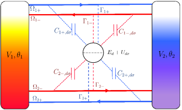
Figure 1: (Color online) Schematics of our setup. A quantum spin Hall bar with a single-level antidot at the center is attached to two terminals, where both voltage bias and temperature gradient are applied. Interactions are described using capacitance coefficients $C_{is,d\sigma}$, where $i=1,2$ labels the edges, $s=\pm$ is the helicity, $d$ stands for dot, and $\sigma=\uparrow,\downarrow$ is the electronic spin. Couplings between the helical edge states and the dot are denoted with $\Gamma_{is}$.

Our aim here is to show that spin-polarized currents can be generated in quantum spin Hall antidot systems using thermal gradients only. In fact, we demonstrate below that pure spin currents and pure spin heat flows can be produced by thermoelectric means (Seebeck and Peltier effects). These effects are relevant because many topological insulators show excellent thermoelectric properties.muc13 For instance, porous three-dimensional topological insulators display large thermoelectric figures of merittre11 and similar properties have been associated to edge conduction channelstak10 and nanowires.goo14 Moreover, spin Nernst signals can provide spectroscopic information in quantum spin Hall devices.rot12 Here, we consider a simple setup: a two-dimensional topological insulator connected to two electronic reservoirs, see Fig. 1. The central antidot allows scattering between helical states in different edges, these transitions preserving the spins of the carriers. Therefore, in the linear regime of transport and for normal conductors the spin current is zero. However, in the nonlinear regime the screening potential in the dot region becomes spin dependent since, quite generally, the dot level will be asymmetrically coupled to the edge states. As a consequence, the nonlinear current will be spin polarized. This makes the nonlinear regime of quantum thermoelectric transport quite unique and interesting to explore, as recently emphasized in Refs. san13, ; whi13, ; mea13, ; lop13, ; her13, ; hwa13, ; mat13, ; bed13, ; fah13, ; dut13, ; whi14, .

Heat currents can also become spin polarized, and we find a spin Peltier effectgra06 ; flip12 in addition to a spin Seebeck effect.Uchida ; jaw10 ; sla10 Rectification effects are more visible in the heat flow,seg05 ; cha06 ; ruo11 which results in strongly asymmetric spin polarizations. We stress that the spin-filter effects discussed here exist regardless of couplings to ferromagnetic contacts or external magnetic (Zeeman) fields (cf. Refs. ted71, ; mes94, ; bre11, ; jan12, ; Vera13, ), and are thereby of purely spintronicfab07 (or spin caloritronic)bau10 character. Furthermore, the spin polarization for both charge and heat currents can be controlled in our system by adjusting the antidot resonant level or changing the background temperature.

The paper is organized as follows. In Sec. II, we describe our model based on scattering theory to determine the generalized transmission probability that depends on the screening potential. Intriguingly, the potential response in the antidot region is spin-dependent even though the contacts are normal leads [Eqs. (9) and (10)], giving rise to spin-polarized electronic and heat currents [Eqs. (17) and (18)], with the asymmetric tunneling described by the parameter $\eta$. The transport coefficients are calculated in Sec. III using an expansion around the equilibrium point. We analytically show that the leading-order rectification terms of the currents with respect to voltage and thermal biases show spin-dependent screening effects, in contrast to the linear coefficients. These results are central to our work. Section IV presents numerical results that are valid beyond the Sommerfeld and the weakly nonlinear approximations when both voltage and thermal biases applied to the sample are strong. We also discuss the possibility of generating pure spin currents from the combination of Seebeck effect and helical propagation in the nonlinear regime of transport. Finally, our conclusions are contained in Sec. V.

II Theoretical model

We consider a quantum spin Hall (QSH) bar attached to two terminals $\alpha=1,2$, where each terminal is driven by the electrical voltage bias $eV_{\alpha}=\mu_{\alpha}-E_{F}$ ($\mu_{\alpha}$ is the electrochemical potential and $E_{F}$ is the common Fermi energy) and also by the temperature shift $\theta_{\alpha}=T_{\alpha}-T$ ($T_{\alpha}$ and $T$ are the lead and the background temperature, respectively), see Fig. 1. An antidot is formed inside the QSH bar. It can connect upper and lower gapless helical edge states. Scattering off the dot is described with the matrix $s_{\alpha\beta}=s_{\alpha\beta}(E,eU)$, which is generally a function of the carrier energy $E$ and the electrostatic potential $U$ inside the system.but93 ; chr96 The potential $U_{\sigma}=U(\vec{r},\{V_{\gamma}\},\{\theta_{\gamma}\},\sigma)$ is, in turn, a function of the position $\vec{r}$, the set of driving fields $\{V_{\gamma}\}$ and $\{\theta_{\gamma}\}$,san13 ; mea13 ; lop13 and the spin index $\sigma=\uparrow,\downarrow$. The $\sigma$-dependence of $U_{\sigma}$ becomes crucial in our QSH system due to the underlying helicity, i.e., the spin-channel separation of charge carriers according to their motion. As a matter of fact, the different response of screening potential through the antidot with respect to each spin-component is the working principle for our observed spin-polarized electric and heat currents since these fluxes are determined by the spin-dependent potential response.

More specifically, the charge and heat currents at lead $\alpha$ carried by spin-component $\sigma$ are respectively given bybut90

$$I_{\alpha}^{\sigma}=\frac{e}{h}\sum_{\beta}\int dEA_{\alpha\beta}^{\sigma}(E,eU)f_{\beta}(E),$$ (1)

$${\cal J}_{\alpha}^{\sigma}=\frac{1}{h}\sum_{\beta}\int dE(E-\mu_{\alpha})A_{\alpha\beta}^{\sigma}(E,eU)f_{\beta}(E),$$ (2)

where $A_{\alpha\beta}^{\sigma}=\text{Tr}[\delta_{\alpha\beta}-s_{\alpha\beta}^{\dagger}s_{\alpha\beta}]$ and $f_{\beta}(E)=(1+\exp[(E-\mu_{\beta})/k_{B}T_{\beta}])^{-1}$ is the Fermi-Dirac distribution function in the reservoir $\beta=1,2$. Note here that we have generalized the expressions for charge and heat currents into their spin-resolved form, for which we separate $2A_{\alpha\beta}$ in the usual current expressionslop13 $I_{\alpha}=(2e/h)\sum_{\beta}\int dEA_{\alpha\beta}(E,eU)f_{\beta}(E)$ and ${\cal J}_{\alpha}=(2/h)\sum_{\beta}\int dE(E-\mu_{\alpha})A_{\alpha\beta}(E,eU)f_{\beta}(E)$ into $A_{\alpha\beta}^{\uparrow}=A_{\alpha\beta}(U_{\uparrow})$ and $A_{\alpha\beta}^{\downarrow}=A_{\alpha\beta}(U_{\downarrow})$ in order to explicitly incorporate the spin-dependent screening effect.

Due to current conservation for respective $\sigma$ and neglecting spin-flip scattering,Ste14 one has $\sum_{\alpha}I_{\alpha}^{\sigma}=0$ and $\sum_{\alpha}({\cal J}_{\alpha}^{\sigma}+I_{\alpha}^{\sigma}V_{\alpha})=0$, and one can define the direction of spin-resolved currents: $I_{\sigma}\equiv I_{1}^{\sigma}=-I_{2}^{\sigma}$ and ${\cal J}_{\sigma}\equiv{\cal J}_{1}^{\sigma}=-{\cal J}_{2}^{\sigma}-I_{\sigma}(V_{1}-V_{2})$. With this convention, we define the spin-polarized currents

$$I_{s} =I_{\uparrow}-I_{\downarrow}$$ (3)

$${\cal J}_{s} ={\cal J}_{\uparrow}-{\cal J}_{\downarrow}$$ (4)

along with the total fluxes $I_{c}\equiv I_{\uparrow}+I_{\downarrow}$ and ${\cal J}_{c}\equiv{\cal J}_{\uparrow}+{\cal J}_{\downarrow}$ (charge and heat, respectively).

The screening potential $U=\sum_{\sigma}U_{\sigma}$ is sensitive to variations of the external voltage or temperature biases. Since our theory is based on an expansion around the equilibrium point, it suffices to expand the potential up to linear order in the driving fields,san13 ; mea13 ; lop13

$$U=U_{\text{eq}}+\sum_{\alpha,\sigma}u_{\alpha\sigma}V_{\alpha}+\sum_{\alpha,\sigma}z_{\alpha\sigma}\theta_{\alpha},$$ (5)

where $u_{\alpha\sigma}=(\partial U_{\sigma}/\partial V_{\alpha})_{\text{eq}}$ and $z_{\alpha\sigma}=(\partial U_{\sigma}/\partial\theta_{\alpha})_{\text{eq}}$ are spin-dependent characteristic potentials (CPs) that relate the variation of the spin-dependent potential $U_{\sigma}$ to voltage and temperature shifts at terminal $\alpha=1,2$.

We treat electron-electron interactions within a mean-field approximation. The self-consistent determination of $U$ can thus be achieved by solving the Poisson equation $\nabla^{2}\Delta U=-4\pi q$, with $\Delta U=U-U_{\text{eq}}=\sum_{\sigma}\Delta U_{\sigma}$ and

$$q=\sum_{\sigma}q_{\sigma}=e\sum_{\alpha,\sigma}\Big{[}D_{\alpha}^{p}(\sigma)eV_{\alpha}+D_{\alpha}^{e}(\sigma)\theta_{\alpha}\Big{]}+e^{2}\sum_{\sigma}\Pi_{\sigma}\Delta U_{\sigma}\,.$$ (6)

The charge pileup $q$ is given by the sum of the bare injected charge determined from the spin-dependent particlebut93 ; chr96 ($p$) and entropicsan13 ($e$) injectivities, $D_{\alpha}^{p,e}(\sigma)=-\int dE\nu_{\alpha}^{p,e}(E,\sigma)\partial_{E}f$, where $\nu_{\alpha}^{p}(E,\sigma)=(2\pi i)^{-1}\sum_{\beta}\text{Tr}\big{[}s_{\beta\alpha}^{\dagger}\frac{ds_{\beta\alpha}}{dE}\big{]}$ and $\nu_{\alpha}^{e}(E,\sigma)=(2\pi i)^{-1}\sum_{\beta}\text{Tr}\big{[}\frac{E-E_{F}}{T}s_{\beta\alpha}^{\dagger}\frac{ds_{\beta\alpha}}{dE}\big{]}$, and the screening charge $e^{2}\sum_{\sigma}\Pi_{\sigma}\Delta U_{\sigma}$, where $\Pi_{\sigma}$ is the spin-dependent Lindhard function which in the long wavelength limit becomes $\Pi_{\sigma}=\int dE\nu_{\sigma}(E)\partial_{E}f$, with $\nu_{\sigma}(E)=\sum_{\alpha}\nu_{\alpha}^{p}(E,\sigma)$ the spin-$\sigma$ electron density of states. Then, the integrated density of states is $D_{\sigma}=\sum_{\alpha}D_{\alpha}^{p}$. Note, however, that possible $\sigma$ dependences of $D_{\alpha}^{p,e}(\sigma)$ and $\Pi_{\sigma}$ would only appear in our model for unequal spin populations arising, e.g., from ferromagnetic contacts. Thus, for normal metallic contacts the only spin-dependent term in Eq. (6) is the screening $\Delta U_{\sigma}$ giving rise to a spin imbalance inside the system.

In the general case, the potential $U(\vec{r})$ is a space-dependent function. For a practical calculation, we discretize the conductor into the regions illustrated in Fig. 1: $\Omega_{is}$, with $i=1,2$ for the upper and lower edges, $s=\pm$ denoting the helicity, and dot region with spin $\sigma$. The edge states are tunnel-coupled to the dot via hybridization widths $\Gamma_{1s}$ and $\Gamma_{2s}$, which explicitly depend on the helicity $s=\pm$ corresponding to spin channels $\uparrow$($+$) and $\downarrow$($-$). The dot is described with a quasilocalized level whose energy $E_{d}$ is controllable by a top gate potential. In the wide-band limit, scattering with the dot is well described using a Breit-Wigner form. Hence, the reflection probability off the dot is given by $r_{\sigma}=1-t_{\sigma}=\Gamma_{1s}\Gamma_{2s}/|\Lambda_{s}|^{2}$, where $\Lambda_{s}=E_{F}-E_{d}+i\Gamma_{s}/2$ with $\Gamma_{s}=\Gamma_{1s}+\Gamma_{2s}$, where $t_{\sigma}$ is the transmission probability. Importantly, the helicity $s$-dependence of $\Gamma_{is}$ ($i=1,2$) disappears for normal contacts, since in this case there is no spin imbalance inside the edge states. This leads to spin-independent transmissions $t_{\uparrow}=t_{\downarrow}$ via antidot scattering. As a consequence, the linear conductance coefficients are spin-independent and the spin-polarization arises only in the nonlinear regime of transport.

The potential $U_{is}$ in each region is assumed to be spatially homogeneous. We describe the Coulomb interaction between the edge states and the dot with a capacitance matrix $C_{is,d\sigma}$.but93 This discrete local potential model captures the essential physics.chr96 ; san04 The region-specific CPs are then given by $u_{i\alpha}^{\sigma}=(\partial U_{i}^{\sigma}/\partial V_{\alpha})_{\text{eq}}$ and $z_{i\alpha}^{\sigma}=(\partial U_{i}^{\sigma}/\partial\theta_{\alpha})_{\text{eq}}$, and the net charge response for each region can be related to the capacitance matrix via

$$q_{is}=e\sum_{\alpha}(D_{is,\alpha}^{p}eV_{\alpha}+D_{is,\alpha}^{e}\theta_{\alpha})+e^{2}\Pi_{is}\Delta U_{is}\\ =\sum_{\sigma}C_{is,d\sigma}(\Delta U_{is}-\Delta U_{d\sigma}).$$ (7)

By solving this, one can determine the potential $U_{i\sigma}=U_{is}$ as a function of the applied voltages and the thermal gradients and obtain the spin-dependent CPs according to Eq. (5) for each spin. It should be noted that the charge with spin $\sigma=\uparrow$($\downarrow$) in the antidot region is supplied from the edge states with helicity $s=+$($-$) via tunnel coupling since we neglect spin-flip processes in order to maximize spin-polarization effects. For definiteness, we assume that the density of states for all regions are equal, i.e., $D_{is}=D_{s}\equiv D/2$, and the injectivities from the two terminals are symmetric, which amount to $D_{is,\alpha}^{p,e}=D_{s}^{p,e}\equiv D^{p,e}/2$ and $\Pi_{is}=\Pi_{s}\equiv\Pi/2$.

We consider the case where the conductor is electrically symmetric, i.e., $C_{is,d\sigma}=C_{is}=C_{s}=C/2$ with $C=C_{+}+C_{-}$, but asymmetric in the scattering properties such that $\Gamma_{1s}=(1+\eta)\Gamma/4$ and $\Gamma_{2s}=(1-\eta)\Gamma/4$ with $\Gamma=\Gamma_{+}+\Gamma_{-}$ ($\Gamma_{s}=\Gamma_{1s}+\Gamma_{2s}=\Gamma/2$). Experimentally, this would be the general situation for dots closer to one of the edge states. Another possibility is to tune the width and the height of the tunnel barriers formed between the resonance and the propagating channels. Thus, the coupling asymmetry is described with a nonzero $\eta=(\Gamma_{1}-\Gamma_{2})/\Gamma$ where $\Gamma_{i}=\sum_{s}\Gamma_{is}$. From Eqs. (5) and (7), we find the dot potential

$$\Delta U_{d\sigma}=u_{1\sigma}V_{1}+u_{2\sigma}V_{2}+z_{1\sigma}\theta_{1}+z_{2\sigma}\theta_{2},$$ (8)

with the corresponding CPs

$$u_{1\uparrow}=u_{2\downarrow}=\frac{1}{2}+\eta c_{\text{sc}},\quad u_{1\downarrow}=u_{2\uparrow}=\frac{1}{2}-\eta c_{\text{sc}},$$ (9)

$$z_{1\uparrow}=z_{2\downarrow}=\frac{D^{e}}{eD^{p}}u_{1\uparrow},\quad z_{1\downarrow}=z_{2\uparrow}=\frac{D^{e}}{eD^{p}}u_{1\downarrow},$$ (10)

where $c_{\text{sc}}=[2-2C/e^{2}\Pi]^{-1}=C_{\mu}/2C$ with $1/C_{\mu}=1/C+1/e^{2}D$ the electrochemical capacitance. Importantly, the CPs become spin-dependent (e.g., $u_{1\uparrow}-u_{1\downarrow}=2\eta c_{\text{sc}}$) whenever $\eta\neq 0$. As a result, we expect electronic transport to be spin polarized for asymmetric couplings. Interestingly, the strength of the CPs polarization is determined by the ratio $C_{\mu}/C$, similarly to the interaction induced magnetic field asymmetry in nonlinear mesoscopic transport.but05 In other words, our effect has a pure interaction origin and vanishes in the noninteracting limit ($C\to\infty$).

The spin dependence of the nonequilibrium potential response can be easily understood in the following way. Suppose that the left voltage is lifted with an amount $\Delta V$ while the right voltage remains unchanged. Then, both the upper edge with $s=+$ and the lower edge state with $s=-$ carry more charge than their counterparts. Since the dot is, say, more coupled to the upper edge than to the lower one, effectively more electrons with spin $\uparrow$ are injected into the dot than electrons with spin $\downarrow$. We emphasize that this effect will be visible in the nonlinear regime of transport only since the linear response coefficients are independent of the CPs in Eqs. (9) and (10).

III Weakly nonlinear transport

In order to illustrate the mechanism of spin polarization for the currents, we firstly focus on the weakly nonlinear regime of transport and expand the electronic and heat currents in Eqs. (1) and (2) around the equilibrium state, $\mu_{\alpha}=E_{F}$ and $T_{\alpha}=T$, up to second order in the driving fields, $V_{\alpha}$ and $\theta_{\alpha}$:san13 ; mea13 ; lop13

$$I_{\alpha}^{\sigma}=\sum_{\beta}\Big{(}G_{\alpha\beta}^{\sigma}V_{\beta}+L_{\alpha\beta}^{\sigma}\theta_{\beta}\Big{)}\\ +\sum_{\beta\gamma}\Big{(}G_{\alpha\beta\gamma}^{\sigma}V_{\beta}V_{\gamma}+L_{\alpha\beta\gamma}^{\sigma}\theta_{\beta}\theta_{\gamma}+2M_{\alpha\beta\gamma}^{\sigma}V_{\beta}\theta_{\gamma}\Big{)},$$ (11)

$${\cal J}_{\alpha}^{\sigma}=\sum_{\beta}\Big{(}R_{\alpha\beta}^{\sigma}V_{\beta}+K_{\alpha\beta}^{\sigma}\theta_{\beta}\Big{)}\\ +\sum_{\beta\gamma}\Big{(}R_{\alpha\beta\gamma}^{\sigma}V_{\beta}V_{\gamma}+K_{\alpha\beta\gamma}^{\sigma}\theta_{\beta}\theta_{\gamma}+2H_{\alpha\beta\gamma}^{\sigma}V_{\beta}\theta_{\gamma}\Big{)}.$$ (12)

These general multi-terminal expressions can easily be applied to our two-terminal setup. In Appendix A, we explicitly write down compact expressions using a Sommerfeld expansion for illustrative purposes, even though this expansion is valid for low temperatures only. Below, we shall numerically evaluate the currents by directly integrating Eqs. (1) and (2) and compare with the analytic results.

Controlled edge backscattering across the dot is given by the transmission probability $t(E_{F})=16(E_{F}-E_{d})^{2}/[16(E_{F}-E_{d})^{2}+\Gamma^{2}]$, which is a spin-independent function since $\Gamma_{1s}=\Gamma_{1}/2$, $\Gamma_{2s}=\Gamma_{2}/2$. Hence, all linear responses are also spin-independent, i.e., $G_{\alpha\beta}^{\uparrow}=G_{\alpha\beta}^{\downarrow}$, $L_{\alpha\beta}^{\uparrow}=L_{\alpha\beta}^{\downarrow}$, $R_{\alpha\beta}^{\uparrow}=R_{\alpha\beta}^{\downarrow}$, and $K_{\alpha\beta}^{\uparrow}=K_{\alpha\beta}^{\downarrow}$ ($\alpha,\beta=1,2$), as should be [see Eqs. (29), (30), (31), and (32)]. This is a straightforward consequence of the fact that linear coefficients are independent of the screening potential. Therefore, spin polarization effects arise in the nonlinear regime of transport only, since nonlinear responses are functions of the CPs and these can exhibit spin asymmetries, e.g., $G_{111}^{\uparrow}\neq G_{111}^{\downarrow}$ with a nonzero $\eta$. This is clear when we substitute Eq. (9) into Eq. (33a).

Hence, in the presence of both voltage and thermal biases with $V_{1}=V$, $V_{2}=0$, $\theta_{1}=\theta$, and $\theta_{2}=0$, the spin-polarized electronic and heat currents read

$$I_{s}=\big{[}G_{111}^{\uparrow}-G_{111}^{\downarrow}\big{]}V^{2}+\big{[}L_{111}^{\uparrow}-L_{111}^{\downarrow}\big{]}\theta^{2}\\ +2\big{[}M_{111}^{\uparrow}-M_{111}^{\downarrow}\big{]}V\theta,$$ (13)

$${\cal J}_{s}=\big{[}R_{111}^{\uparrow}-R_{111}^{\downarrow}\big{]}V^{2}+\big{[}K_{111}^{\uparrow}-K_{111}^{\downarrow}\big{]}\theta^{2}\\ +2\big{[}H_{111}^{\uparrow}-H_{111}^{\downarrow}\big{]}V\theta.$$ (14)

We emphasize that the effects discussed in this work remain the same even if we consider different types of bias configurations such as $V_{1}=V/2$, $V_{2}=-V/2$, $\theta_{1}=-\theta/2$, $\theta_{2}=\theta/2$, which, however, only complicate the algebra within our context.

The ordinary charge and heat currents are written by

$$I_{c}=\big{[}G_{11}^{\uparrow}+G_{11}^{\downarrow}\big{]}V+\big{[}L_{11}^{\uparrow}+L_{11}^{\downarrow}\big{]}\theta+\big{[}G_{111}^{\uparrow}+G_{111}^{\downarrow}\big{]}V^{2}\\ +\big{[}L_{111}^{\uparrow}+L_{111}^{\downarrow}\big{]}\theta^{2}+2\big{[}M_{111}^{\uparrow}+M_{111}^{\downarrow}\big{]}V\theta,$$ (15)

$${\cal J}_{c}=\big{[}R_{11}^{\uparrow}+R_{11}^{\downarrow}\big{]}V+\big{[}K_{11}^{\uparrow}+K_{11}^{\downarrow}\big{]}\theta+\big{[}R_{111}^{\uparrow}+R_{111}^{\downarrow}\big{]}V^{2}\\ +\big{[}K_{111}^{\uparrow}+K_{111}^{\downarrow}\big{]}\theta^{2}+2\big{[}H_{111}^{\uparrow}+H_{111}^{\downarrow}\big{]}V\theta.$$ (16)

Applying the relevant nonlinear coefficients in Appendix A to Eqs. (13) and (14), we find

$$I_{s}=-\frac{e^{3}}{h}(u_{1\uparrow}-u_{1\downarrow})t^{\prime}V^{2}-\frac{e^{2}\pi^{2}k_{B}^{2}T}{3h}(z_{1\uparrow}-z_{1\downarrow})t^{\prime\prime}\theta^{2}\\ -\frac{e^{3}}{h}\bigg{[}\frac{\pi^{2}k_{B}^{2}T}{3e}(u_{1\uparrow}-u_{1\downarrow})t^{\prime\prime}+(z_{1\uparrow}-z_{1\downarrow})t^{\prime}\bigg{]}V\theta,$$ (17)

$${\cal{J}}_{s}=-\frac{e^{2}\pi^{2}(k_{B}T)^{2}}{3h}(u_{1\uparrow}-u_{1\downarrow})t^{\prime\prime}V^{2}-\frac{e\pi^{2}k_{B}^{2}T}{3h}(z_{1\uparrow}-z_{1\downarrow})t^{\prime}\theta^{2}\\ -\frac{e^{2}\pi^{2}(k_{B}T)^{2}}{3h}\bigg{[}\frac{1}{eT}(u_{1\uparrow}-u_{1\downarrow})t^{\prime}+(z_{1\uparrow}-z_{1\downarrow})t^{\prime\prime}\bigg{]}V\theta,$$ (18)

where $t\equiv t(E_{F})$, $t^{\prime}\equiv\partial_{E}t(E)|_{E=E_{F}}$, and $t^{\prime\prime}\equiv\partial^{2}_{E}t(E)|_{E=E_{F}}$. These expressions are central to our results. The spin-polarized electronic and heat currents indeed appear when the potential response via antidot scattering is different with respect to each spin component, i.e., either $u_{1\uparrow}-u_{1\downarrow}\neq 0$ or $z_{1\uparrow}-z_{1\downarrow}\neq 0$. Using the CPs in Eqs. (9) and (10) explicitly, one can finally write

$$I_{s}=-\eta c_{\text{sc}}\bigg{(}\frac{2e^{3}}{h}t^{\prime}V^{2}+\frac{2e\pi^{2}k_{B}^{2}T}{3h}\frac{D^{e}}{D^{p}}t^{\prime\prime}\theta^{2}\\ +\frac{2e^{2}}{h}\bigg{[}\frac{\pi^{2}k_{B}^{2}T}{3}t^{\prime\prime}+\frac{D^{e}}{D^{p}}t^{\prime}\bigg{]}V\theta\bigg{)},$$ (19)

$${\cal{J}}_{s}=-\eta c_{\text{sc}}\bigg{(}\frac{2e^{2}\pi^{2}(k_{B}T)^{2}}{3h}t^{\prime\prime}V^{2}+\frac{2\pi^{2}k_{B}^{2}T}{3h}\frac{D^{e}}{D^{p}}t^{\prime}\theta^{2}\\ +\frac{2e\pi^{2}(k_{B}T)^{2}}{3h}\bigg{[}\frac{1}{T}t^{\prime}+\frac{D^{e}}{D^{p}}t^{\prime\prime}\bigg{]}V\theta\bigg{)}.$$ (20)

Note that the spin-polarization of both currents is directly proportional to the asymmetry parameter $\eta$ and the interaction parameter $c_{\text{sc}}$. Hence, the asymmetrically coupled quantum antidot plays the role of a spin filter. In contrast, as shown in Eqs. (15) and (16), the effect of the potential response on the usual electronic and heat currents can be represented by the sum $u_{1\uparrow}+u_{1\downarrow}$ and $z_{1\uparrow}+z_{1\downarrow}$ rather than the difference. Due to helicity, we have $u_{1\uparrow}+u_{1\downarrow}=1$ and $z_{1\uparrow}+z_{1\downarrow}=D^{e}/eD^{p}$ from Eqs. (9) and (10), independently of the asymmetry:

$$I_{c}=\frac{2e^{2}}{h}tV+\frac{2e\pi^{2}k_{B}^{2}T}{3h}t^{\prime}\theta+\frac{e\pi^{2}k_{B}^{2}}{3h}\bigg{(}t^{\prime}-T\frac{D^{e}}{D^{p}}t^{\prime\prime}\bigg{)}\theta^{2}\\ +\frac{e^{2}}{h}\bigg{(}\frac{\pi^{2}k_{B}^{2}T}{3}t^{\prime\prime}-\frac{D^{e}}{D^{p}}t^{\prime}\bigg{)}V\theta,$$ (21)

$${\cal{J}}_{c}=\frac{2e\pi^{2}(k_{B}T)^{2}}{3h}t^{\prime}V+\frac{2\pi^{2}k_{B}^{2}T}{3h}t\theta-\frac{e^{2}}{h}\bigg{(}t+\frac{\pi^{2}(k_{B}T)^{2}}{6}t^{\prime\prime}\bigg{)}V^{2}\\ +\frac{\pi^{2}k_{B}^{2}}{3h}\bigg{(}t-T\frac{D^{e}}{D^{p}}t^{\prime}\bigg{)}\theta^{2}+\frac{e\pi^{2}k_{B}^{2}T}{3h}\bigg{(}t^{\prime}-T\frac{D^{e}}{D^{p}}t^{\prime\prime}\bigg{)}V\theta.$$ (22)

Remarkably, the second-order electric response $G_{111}^{\uparrow}+G_{111}^{\downarrow}$ cancels out because this term contains the screening effect with a factor $1-(u_{1\uparrow}+u_{1\downarrow})$ [Eq. (33a)], which is always zero for normal contacts due to helical nature of the edge states. It should be emphasized that this cancellation is not originated from our specific bias setup $V_{1}=V,~{}V_{2}=0$. Indeed, even for a general voltage bias configuration, i.e., $V_{1}=\xi V$ and $V_{2}=(\xi-1)V$ with $0\leq\xi\leq 1$, the second order effect of voltage driving can be written as $\sum_{\sigma}G_{111}^{\sigma}(V_{1}-V_{2})^{2}=\sum_{\sigma}G_{122}^{\sigma}(V_{1}-V_{2})^{2}=-\sum_{\sigma}G_{211}^{\sigma}(V_{1}-V_{2})^{2}=0$, due to gauge invariance and current conservation. Therefore, the charge current in the isothermal case, i.e., $\theta_{1}=\theta_{2}=0$, is always given by $I_{c}=(2e^{2}/h)tV$ up to order $V^{3}$. This absence of rectification effects in our two-dimensional topological insulator system is in stark contrast with small conductors coupled to normal reservoirs, in which the $V^{2}$ term is generally present.son98 ; lin00 ; sho01 ; fle02 ; but03 ; gon04 ; hac04 ; seg05

IV Numerical results

In the previous section, we discussed the underlying spin-filter mechanism in an intuitive way, deriving expressions valid in the weakly nonlinear regime, as shown in Eqs. (17) and (18). These analytic results are also based on a Sommerfeld expansion, which is appropriate at low temperatures. To extend the validity of our conclusions for both strong nonlinearities and high temperatures, we now evaluate the currents numerically via direct integration of Eqs. (1) and (2) without any further assumption. Our only limitation is the mean-field approximation, thus neglecting strong electron-electron correlations in our system. Below, we discuss the isothermal ($\theta_{1}=\theta_{2}=0$) and isoelectric ($V_{1}=V_{2}=0$) cases separately. Finally, we consider the general case ($V_{1}=V,\theta_{1}=\theta$) for which, interestingly, pure spin currents can be generated.

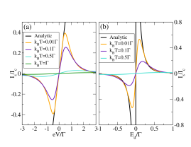
Figure 2: (Color online) Plots of $I_{s}/I_{c}$ versus (a) voltage bias $eV/\Gamma$ at $E_{d}/\Gamma=0.25$ and (b) antidot level $E_{d}/\Gamma$ at $eV/\Gamma=0.25$, for several background temperatures $k_{B}T$ in the isothermal case. In all cases, we use $\eta=c_{\text{sc}}=0.5$ and $E_{F}=0$.

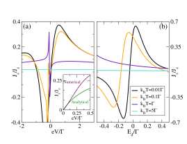
Figure 3: (Color online) Plots of ${\cal{J}}_{s}/{\cal{J}}_{c}$ versus (a) voltage bias $eV/\Gamma$ at $E_{d}/\Gamma=0.2$ and (b) antidot level $E_{d}/\Gamma$ at $eV/\Gamma=0.25$, for several background temperatures $k_{B}T$ in the isothermal case. In the inset of (a), an analytic result is shown in comparison with the numerical one at $k_{B}T/\Gamma=0.1$. Parameters used are $\eta=c_{\text{sc}}=0.5$. Note that since at moderate voltages the Joule heating present in $\mathcal{J}_{c}$ dominates the spin heat flow quickly becomes a nonlinear function of $V$.

IV.1 Voltage-driven transport: isothermal case

In Fig. 2(a), we plot the dimensionless ratio $I_{s}/I_{c}$ between the spin-polarized current and the charge flux as a function of the voltage bias $V$ for a given antidot level position $E_{d}$. At low voltages, we observe a linear dependence of $I_{s}/I_{c}$ with $V$, in agreement with the analytical results. We note that for $\theta_{1}=\theta_{2}=0=V_{2}$ and $V_{1}=V$, the spin-polarized current in Eq. (19) reduces to

$$I_{s}=-\frac{2e^{3}}{h}\eta c_{\text{sc}}t^{\prime}V^{2}\,,$$ (23)

while the charge current is simply given by $I_{c}=(2e^{2}/h)tV$, both to leading order in a voltage expansion for low $T$. Therefore, the degree of polarization $I_{s}/I_{c}$ increases with voltage for small $V$. At higher voltages, the polarization decreases when $V$ is larger than $\Gamma/e$ because charge fluctuations are quenched. In Fig. 2(b), we show the gate tuning of $I_{s}/I_{c}$, which is depicted for a fixed bias. Again, the maximal polarization is attained when the dot level is above or below the Fermi energy on the scale of the hybridization width $\Gamma$ because Eq. (23) shows that the spin current is proportional to $t^{\prime}$, which is a function with an energy dependence governed by $\Gamma$ in the Breit-Wigner approximation. Furthermore, our results show that the polarization decreases when the background temperature $T$ increases since large temperatures tend to smear out the energy dependence of the scattering matrix, an essential ingredient of our spin-filter effect.

Figure 3(a) displays the spin polarization of the heat current, defined as ${\cal{J}}_{s}/{\cal{J}}_{c}$, as a function of the bias voltage. For small $V$ in the isothermal case, Eq. (20) yields

$${\cal{J}}_{s}=-\eta c_{\text{sc}}(2e^{2}\pi^{2}/3h)(k_{B}T)^{2}t^{\prime\prime}V^{2}\,.$$ (24)

This can be seen as the leading-order spin-polarizedgra06 nonlinear Peltier effect.kul94 ; bog99 ; zeb07 In turn, the heat flux associated to charge transport is given, to lowest order in $V$, by ${\cal{J}}_{c}=(2e\pi^{2}/3h)(k_{B}T)^{2}t^{\prime}V-(e^{2}/h)[t+(\pi^{2}/6)(k_{B}T)^{2}t^{\prime\prime}]V^{2}$ [we set $\theta_{1}=\theta_{2}=0=V_{2}$ and $V_{1}=V$ in Eq. (22)], where the conventional Peltier coefficient and the Joule heating term are clearly shown. Since the latter dominates even at low $V$, the spin polarization quickly departs from the linear dependence, see the inset of Fig. 3(a). Moreover, we observe an asymmetry between positive and negative voltages due to the heat current being, in general, asymmetric with respect to energy integration due to the $\mu=E_{F}+eV$ term in Eq. (2). Recent experiments with scanning tunneling microscope probes coupled to molecules attached to substrate precisely observe an asymmetric heat dissipation in the charge sector.lee13 Here, we predict that the same phenomenon will occur for the spin degree of freedom and that it can be manipulated either changing the base temperature or the dot level position, see Fig. 3(b).

IV.2 Temperature-driven transport: isoelectric case

We now consider the case of an applied temperature bias such as $\theta_{1}=\theta$ and $\theta_{2}=0$ for equal electrochemical potentials $V_{1}=V_{2}=0$. To leading order in a $\theta$ expansion, the spin-dependent current becomes at low $T$

$$I_{s}=-\eta c_{\text{sc}}(2e\pi^{2}k_{B}^{2}T/3h)(D^{e}/D^{p})t^{\prime\prime}\theta^{2}\,.$$ (25)

Similarly to the isothermal case [cf. Eq. (23)], the spin current is purely nonlinear in the driving field. Nevertheless, unlike the isothermal case $I_{s}$ in the isoelectric case depends not only on the particle injectivity but also on the entropic contribution since the temperature dependence of the transmission is determined, to leading order, by the carrier energy measured with regard to $E_{F}$.san13 We also note that $I_{s}$ vanishes if the background temperature $T$ tends to zero, thereby our thermal spin generation has a thermoelectric character like the spin Seebeck effect.Uchida ; jaw10 ; sla10 In fact, the charge current is simply given by the thermocurrent expression $I_{c}=(2e\pi^{2}k_{B}^{2}T/3h)t^{\prime}\theta$ up to $\mathcal{O}(\theta)$. Hence, the spin-polarization ratio $I_{s}/I_{c}$ is a linear function of $\theta$ at low $\theta$. This is confirmed with our numerical results in Fig. 4(a). In Fig. 4(b) we show that the spin-filter effect can be, to a large extent, tuned with a gate voltage for a fixed value of $\theta$, which can even reverse the sign of $I_{s}/I_{c}$. In contrast to the isothermal case, the spin polarization degree vanishes for very low temperatures except for $E_{d}$ close to the leads’ Fermi energy. It is precisely at this energy for which the isoelectric $I_{s}$ is more sensitive to changes in $\theta$, in agreement with Eq. (25).

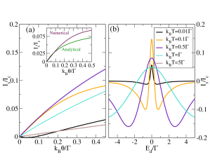
Figure 4: (Color online) Plots of $I_{s}/I_{c}$ versus (a) thermal gradients $k_{B}\theta/\Gamma$ at $E_{d}/\Gamma=0.2$ and (b) antidot level $E_{d}/\Gamma$ at $k_{B}\theta/\Gamma=0.25$, for several background temperatures $k_{B}T$ in the isoelectric case. In the inset of (a), an analytic result is shown in comparison with the numerical one at $k_{B}T/\Gamma=0.1$. We use $\eta=c_{\text{sc}}=0.5$ and $E_{F}=0$.

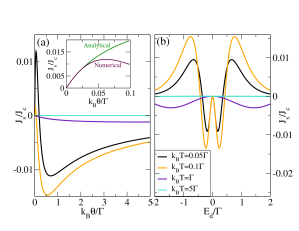
Figure 5: (Color online) Plots of $\mathcal{J}_{s}/\mathcal{J}_{c}$ versus (a) thermal gradients $k_{B}\theta/\Gamma$ at $E_{d}/\Gamma=0.3$ and (b) antidot level $E_{d}/\Gamma$ at $k_{B}\theta/\Gamma=0.25$, for several background temperatures $k_{B}T$ in the isoelectric case. In the inset of (a), an analytic result is shown in comparison with the numerical one at $k_{B}T/\Gamma=0.05$. We use $\eta=c_{\text{sc}}=0.5$ and $E_{F}=0$.

The heat current can also become spin polarized upon the application of a thermal gradient because the generalized thermal conductance depends on the spin index, see Eq. (37). For $\theta_{1}=\theta$ and $V_{1}=V_{2}=0=\theta_{2}$ we find

$${\cal{J}}_{s}=-\eta c_{\text{sc}}(2\pi^{2}k_{B}^{2}T/3h)(D^{e}/D^{p})t^{\prime}\theta^{2}$$ (26)

to leading order in the temperature bias. The heat current due to charge transport is given by ${\cal{J}}_{c}=(2\pi^{2}k_{B}^{2}T/3h)t\theta+\mathcal{O}(\theta)^{2}$ at low $T$. Therefore, the ratio ${\cal{J}}_{s}/{\cal{J}}_{c}$ is generally nonzero for increasing $\theta$, see Fig. 5(a). Interestingly, at resonance ($E_{d}=E_{F}$) the spin polarization of the heat current becomes zero [Fig. 5(b)] while the electric current counterpart shows a local maximum [Fig. 4(b)], indicating that the spin-filter mechanism of a QSH antidot acts differently to electric and heat currents.

IV.3 Thermoelectric transport: pure spin currents

We have shown above that thermal gradients can generate spin-polarized thermocurrents $I_{s}\neq 0$, as a synergistic combination of thermoelectric and spintronic effects.Uchida ; jaw10 ; sla10 We now prove that it is even possible to create pure spin currents, i.e., $I_{s}\neq 0$ for vanishingly small charge current, $I_{c}=0$. The latter condition can be easily achieved in open-circuit conditions, in which case a thermovoltage $V_{\text{th}}$ is generated in response to a temperature bias $\theta$. In Fig. 6(a) we plot the numerically calculated set of biases $\{\theta,V\}$ which satisfy the expression $I_{c}(V_{\text{th}},\theta)=0$ as a function of $\theta$. As expected, at low temperature bias the thermovoltage shows a linear dependence because the Seebeck coefficient, $S=V_{\text{th}}/\theta$, is constant for small thermal gradients. With increasing $\theta$, the thermovoltage acquires a nonlinear component.san13 ; fah13

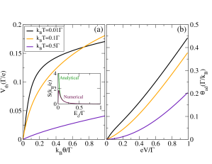
Figure 6: (Color online) Plots of generated (a) thermovoltage $V_{\text{th}}$ versus applied thermal gradient $k_{B}\theta/\Gamma$ and (b) adiabatic thermal gradient $\theta_{\text{ad}}$ versus voltage bias $eV/\Gamma$, at $E_{d}=0.1\Gamma$ for several background temperatures $k_{B}T$. In the inset of (a), the Seebeck coefficient with analytic and numerical results at $k_{B}T=0.01\Gamma$ are shown as a function of resonance level $E_{d}/\Gamma$. Parameters are $\eta=c_{\text{sc}}=0.5$ and $E_{F}=0$.

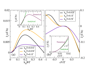
Figure 7: (Color online) Plots of (a) pure spin currents $I_{s}$ versus thermal gradient $k_{B}\theta/\Gamma$ and (b) pure spin heat currents ${\cal{J}}_{s}$ versus voltage bias $eV/\Gamma$, at $E_{d}/\Gamma=0.25$ for several background temperatures $k_{B}T$. The insets compare the analytic and numerical results at (a) $k_{B}T=0.03\Gamma$ and (b) $k_{B}T=0.02\Gamma$, where the latter comparision has been made in a very small bias range where ${\cal{J}}_{s}$ is positive. We use $\eta=c_{\text{sc}}=0.5$ and $E_{F}=0$.

Substituting $V$ with $V_{\rm th}(\theta)$ in the expression for $I_{s}$ we find the pure spin current

$$I_{s}=\eta c_{\text{sc}}\frac{2e\pi^{2}k_{B}^{2}T}{3h}\Bigg{(}\frac{\pi^{2}k_{B}^{2}T}{3}\bigg{[}\frac{t^{\prime}t^{\prime\prime}}{t}-\frac{(t^{\prime})^{3}}{t^{2}}\bigg{]}\\ +\frac{D^{e}}{D^{p}}\bigg{[}\frac{(t^{\prime})^{2}}{t}-t^{\prime\prime}\bigg{]}\Bigg{)}\theta^{2},$$ (27)

up to leading order in $\theta$. Figure 7(a) shows the numerical results for pure $I_{s}$ beyond the quadratic regime (the inset displays a comparison with the analytical results). We observe that the amplitude of $I_{s}$ firstly increases as $T$ is enhanced (here, it is shown from $k_{B}T/\Gamma=0.01$ to $k_{B}T/\Gamma=0.03$) and then decreases (from $k_{B}T/\Gamma=0.03$ to $k_{B}T/\Gamma=0.1$), exhibiting a nonmonotonic behavior with $T$.

Our device also creates pure spin heat flows using electric means only. We first solve the equation ${\cal{J}}_{c}(V,\theta_{\text{ad}})=0$, which amounts to adiabatically isolating the sample. This yields a generated thermal bias $\theta_{\text{ad}}$ in response to the applied voltage $V$, see Fig. 6(b). $\theta_{\text{ad}}$ is an increasing function of $V$ since a positive thermal gradient compensates the current flowing through the system. The effect is less pronounced for higher background temperatures $T$ because more electrons become thermally excited for increasing $T$. We then substitute $\theta_{\text{ad}}(V)$ in the ${\cal{J}}_{s}$ expression and find,

$${\cal{J}}_{s}=\eta c_{\text{sc}}\frac{2e^{2}\pi^{2}(k_{B}T)^{2}}{3h}\Bigg{(}\bigg{[}\frac{(t^{\prime})^{2}}{t}-t^{\prime\prime}\bigg{]}\\ +T\frac{D^{e}}{D^{p}}\bigg{[}\frac{t^{\prime}t^{\prime\prime}}{t}-\frac{(t^{\prime})^{3}}{t^{2}}\bigg{]}\Bigg{)}V^{2}.$$ (28)

up to leading order in $V$. We plot in Fig. 7(b) the pure spin heat current ${\cal{J}}_{s}$ as a function of the bias voltage. At low $V$, our numerical results agree with Eq. (28) (see the inset). For higher voltage, the results are also in qualitative agreement with $I_{s}$ because $|{\cal{J}}_{s}|$ increases to higher values of $T$ (here it is shown up to $k_{B}T/\Gamma=0.1$), beyond which the amplitude of ${\cal{J}}_{s}$ starts to decrease.

V Conclusions

Two-dimensional topological insulators with controlled backscattering present a rich spin dynamics which can be manipulated with external gate potentials and background temperatures. We have demonstrated that spin-polarized currents can be generated in a two-terminal quantum spin Hall systems coupled to normal contacts. Neither Zeeman fields nor ferromagnetic materials are needed in the implementation of our effect. The spin dependence is purely induced by interactions and arises in the nonequilibrium screening potential of the conductor in the response to either voltage or temperature shifts applied to the contacts. Importantly, pure spin currents can be created using the Seebeck effect. The spin-polarization mechanism also works for the heat current, in which case a pure spin heat flow is generated for adiabatically isolated samples.

Our discussion ignores spin-flip processes and Coulomb blockade effects. The former will be detrimental to our spin filtering operational principle if spin-flip transitions preserve the momentum.Ste14 The latter will have a less clear effect. Our theory shows that the screening potential becomes spin-independent in the noninteracting limit, i.e., $C\to\infty$ in Eqs. (9) and (10). The spin-filtering effect becomes stronger as $C\to 0$. Therefore, strong interaction would favor the generation of spin currents and single charge effects are expected to maintain the effects discovered in our work. However, if Coulomb blockade allows the spin-flip transitions, a more careful analysis should be performed. Spin-increasing and spin-decreasing transitions have been experimentally reported.pot03 In addition, the impact of spin-blockade phenomenaono02 deserves further investigation.

In general, there is considerable scope to extend our model and treat different situations. For instance, one could consider the competition between the spin-polarization effects discussed here and spin filtering inherent to ferromagnetic contacts or Zeeman splittings. Inclusion of these influences in our theoretical model would be straightforward. Another interesting possibility would be the study of the thermodynamic efficiency, a subject of practical importance that has recently attracted a good deal of attention, especially in quantum conductors.ben13

VI Acknowledgments

This research was supported by MINECO under Grant No. FIS2011-23526, the Kavli Institute for Theoretical Physics through NSF grant PHY11-25915 and the National Research Foundation of Korea (NRF) grants funded by the Korea government (MSIP) (No. 2011-0030046).

Appendix A Coefficients in Sommerfeld expansion

In a two-terminal setup ignoring the spin-flip scattering, the current conservation condition gives $A_{11}^{\sigma}=A_{22}^{\sigma}=-A_{12}^{\sigma}=-A_{21}^{\sigma}=t^{\sigma}(E)$ where $t^{\sigma}(E)$ is the spin-dependent transmission probability. One can find linear and nonlinear coefficientssan13 ; lop13 in Eqs. (11) and (12) to leading order of the Sommerfeld expansion:

$$G_{11}^{\sigma}=G_{22}^{\sigma}=-G_{12}^{\sigma}=-G_{21}^{\sigma}=\frac{e^{2}}{h}t^{\sigma}(E_{F}),$$ (29)

$$L_{11}^{\sigma}=L_{22}^{\sigma}=-L_{12}^{\sigma}=-L_{21}^{\sigma}=\frac{e\pi^{2}k_{B}^{2}T}{3h}\frac{\partial t^{\sigma}(E)}{\partial E}\bigg{|}_{E_{F}},$$ (30)

$$R_{11}^{\sigma}=R_{22}^{\sigma}=-R_{12}^{\sigma}=-R_{21}^{\sigma}=\frac{e\pi^{2}(k_{B}T)^{2}}{3h}\frac{\partial t^{\sigma}(E)}{\partial E}\bigg{|}_{E_{F}},$$ (31)

$$K_{11}^{\sigma}=K_{22}^{\sigma}=-K_{12}^{\sigma}=-K_{21}^{\sigma}=\frac{\pi^{2}k_{B}^{2}T}{3h}t^{\sigma}(E_{F}),$$ (32)

$$G_{111}^{\sigma} =\frac{e^{3}}{h}\frac{\partial t^{\sigma}(E)}{\partial E}\bigg{|}_{E_{F}}\bigg{(}\frac{1}{2}-u_{1\sigma}\bigg{)},$$ (33a)

$$G_{122}^{\sigma} =\frac{e^{3}}{h}\frac{\partial t^{\sigma}(E)}{\partial E}\bigg{|}_{E_{F}}\bigg{(}u_{2\sigma}-\frac{1}{2}\bigg{)},$$ (33b)

$$G_{211}^{\sigma} =\frac{e^{3}}{h}\frac{\partial t^{\sigma}(E)}{\partial E}\bigg{|}_{E_{F}}\bigg{(}u_{1\sigma}-\frac{1}{2}\bigg{)},$$ (33c)

$$L_{111}^{\sigma} =\frac{e\pi^{2}k_{B}^{2}}{6h}\bigg{[}\frac{\partial t^{\sigma}(E)}{\partial E}-2ez_{1\sigma}T\frac{\partial^{2}t^{\sigma}(E)}{\partial E^{2}}\bigg{]}_{E_{F}},$$ (34a)

$$L_{122}^{\sigma} =-\frac{e\pi^{2}k_{B}^{2}}{6h}\bigg{[}\frac{\partial t^{\sigma}(E)}{\partial E}-2ez_{2\sigma}T\frac{\partial^{2}t^{\sigma}(E)}{\partial E^{2}}\bigg{]}_{E_{F}},$$ (34b)

$$L_{211}^{\sigma} =-\frac{e\pi^{2}k_{B}^{2}}{6h}\bigg{[}\frac{\partial t^{\sigma}(E)}{\partial E}-2ez_{1\sigma}T\frac{\partial^{2}t^{\sigma}(E)}{\partial E^{2}}\bigg{]}_{E_{F}},$$ (34c)

$$M_{111}^{\sigma} =-\frac{e^{3}}{2h}\bigg{[}\frac{\partial t^{\sigma}(E)}{\partial E}z_{1\sigma}+\frac{\pi^{2}k_{B}^{2}T}{3e}\frac{\partial^{2}t^{\sigma}(E)}{\partial E^{2}}(u_{1\sigma}-1)\bigg{]}_{E_{F}},$$ (35a)

$$M_{121}^{\sigma} =\frac{e^{3}}{2h}\bigg{[}\frac{\partial t^{\sigma}(E)}{\partial E}z_{1\sigma}-\frac{\pi^{2}k_{B}^{2}T}{3e}\frac{\partial^{2}t^{\sigma}(E)}{\partial E^{2}}u_{2\sigma}\bigg{]}_{E_{F}},$$ (35b)

$$R_{111}^{\sigma} =-\frac{e^{2}}{2h}\bigg{[}t^{\sigma}(E)+\frac{\pi^{2}(k_{B}T)^{2}}{6}\frac{\partial^{2}t^{\sigma}(E)}{\partial E^{2}}(4u_{1\sigma}-1)\bigg{]}_{E_{F}},$$ (36a)

$$R_{122}^{\sigma} =-\frac{e^{2}}{2h}\bigg{[}t^{\sigma}(E)+\frac{\pi^{2}(k_{B}T)^{2}}{6}\frac{\partial^{2}t^{\sigma}(E)}{\partial E^{2}}(3-4u_{2\sigma})\bigg{]}_{E_{F}},$$ (36b)

$$R_{211}^{\sigma} =-\frac{e^{2}}{2h}\bigg{[}t^{\sigma}(E)+\frac{\pi^{2}(k_{B}T)^{2}}{6}\frac{\partial^{2}t^{\sigma}(E)}{\partial E^{2}}(3-4u_{1\sigma})\bigg{]}_{E_{F}},$$ (36c)

$$K_{111}^{\sigma} =\frac{\pi^{2}k_{B}^{2}}{6h}\bigg{[}t^{\sigma}(E)-2ez_{1\sigma}T\frac{\partial t^{\sigma}(E)}{\partial E}\bigg{]}_{E_{F}},$$ (37a)

$$K_{122}^{\sigma} =-\frac{\pi^{2}k_{B}^{2}}{6h}\bigg{[}t^{\sigma}(E)-2ez_{2\sigma}T\frac{\partial t^{\sigma}(E)}{\partial E}\bigg{]}_{E_{F}},$$ (37b)

$$K_{211}^{\sigma} =-\frac{\pi^{2}k_{B}^{2}}{6h}\bigg{[}t^{\sigma}(E)-2ez_{1\sigma}T\frac{\partial t^{\sigma}(E)}{\partial E}\bigg{]}_{E_{F}},$$ (37c)

$$H_{111}^{\sigma} =\frac{e^{2}\pi^{2}(k_{B}T)^{2}}{6h}\bigg{[}\frac{1}{eT}\frac{\partial t^{\sigma}(E)}{\partial E}(1-u_{1\sigma})-\frac{\partial^{2}t^{\sigma}(E)}{\partial E^{2}}z_{1\sigma}\bigg{]}_{E_{F}},$$ (38a)

$$H_{121}^{\sigma} =\frac{e^{2}\pi^{2}(k_{B}T)^{2}}{6h}\bigg{[}\frac{1}{eT}\frac{\partial t^{\sigma}(E)}{\partial E}(1-u_{2\sigma})+\frac{\partial^{2}t^{\sigma}(E)}{\partial E^{2}}z_{1\sigma}\bigg{]}_{E_{F}},$$ (38b)

where $t^{\sigma}(E_{F})=1-\Gamma_{1s}\Gamma_{2s}/|\Lambda_{s}|^{2}$ with $\Lambda_{s}=E_{F}-E_{d}+i\Gamma_{s}/2$, $\Gamma_{s}=\Gamma_{1s}+\Gamma_{2s}$, and $s=\pm$ corresponding to $\sigma=\uparrow,\downarrow$ interchangeably.

References

- (1) C. L. Kane and E. J. Mele, Phys. Rev. Lett. 95, 226801 (2005).
- (2) B. A. Bernevig, T. L. Hughes, and S.-C. Zhang, Science 314, 1757 (2006).
- (3) C. L. Kane and E. J. Mele, Phys. Rev. Lett. 95, 146802 (2005).
- (4) L. Sheng, D. N. Sheng, C. S. Ting, and F. D. M. Haldane, Phys. Rev. Lett. 95, 136602 (2005).
- (5) C. Xu and J. E. Moore, Phys. Rev. B 73, 045322 (2006).
- (6) M. König, S. Weidmann, C. Brune, A. Roth, H. Buhmann, L. W. Molenkamp, X.-L. Qi, and S.-C. Zhang, Science 318, 766 (2007).
- (7) A. Roth, C. Brn̈e, H. Buhmann, L. W. Molenkamp, J. Maciejko, X.-L. Qi, and S.-C. Zhang, Science 325, 294 (2009).
- (8) C. Brüne, A. Roth, H. Buhmann, E. M. Hankiewicz, L. W. Molenkamp, J. Maciejko, X.-L. Qi, and S.-C. Zhang, Nature Phys. 8, 485 (2012).
- (9) I. Knez, R.-R. Du, and G. Sullivan, Phys. Rev. Lett. 107, 136603 (2011).
- (10) I. Knez, C. T. Rettner, S.-H. Yang, S. S. P. Parkin, L. Du, R.-R. Du, and G. Sullivan, Phys. Rev. Lett. 112, 026602 (2014).
- (11) F. Dolcini, Phys. Rev. B 83, 165304 (2011).
- (12) V. Krueckl and K. Richter, Phys. Rev. Lett. 107, 086803 (2011).
- (13) R. Citro, F. Romeo, and N. Andrei, Phys. Rev. B 84, 161301(R) (2011).
- (14) F. Romeo, R. Citro, D. Ferraro, and M. Sassetti, Phys. Rev. B 86, 165418 (2012).
- (15) A. A. Sukhanov and V. A. Sablikov, J. Phys.: Condens. Matt. 24, 405301 (2012).
- (16) G. Dolcetto, F. Cavaliere, D. Ferraro, and M. Sassetti, Phys. Rev. B 87, 085425 (2013).
- (17) J. Guo, W. Liao, H. Zhao, and G. Zhou, J. Appl. Phys. 115, 023709 (2014).
- (18) R.-L. Chu, J. Li, J. K. Jain, and S.-Q. Shen, Phys. Rev. B 80, 081102(R) (2009).
- (19) G. Tkachov and E. M. Hankiewicz, Phys. Rev. B 83, 155412 (2011).
- (20) J. M. Edge, J. Li, P. Delplace, and M. Büttiker, Phys. Rev. Lett. 110, 246601 (2013).
- (21) S.-P. Chao, S. A. Silotri, and C.-H. Chung, Phys. Rev. B 88, 085109 (2013).
- (22) R. López, J. S. Lim, and D. Sánchez, Phys. Rev. Lett. 108, 246603 (2012).
- (23) S. Mi, D. I. Pikulin, M. Wimmer, and C. W. J. Beenakker, Phys. Rev. B 87, 241405(R) (2013).
- (24) B. Rizzo, L. Arrachea, and M. Moskalets, Phys. Rev. B 88, 155433 (2013).
- (25) C. Timm, Phys. Rev. B 86, 155456 (2012).
- (26) T. Posske, C.-X. Liu, J. C. Budich, and B. Trauzettel, Phys. Rev. Lett. 110, 016602 (2013).
- (27) M. König, M. Baenninger, A. G. F. Garcia, N. Harjee, B. L. Pruitt, C. Ames, P. Leubner, C. Brüne, H. Buhmann, L. W. Molenkamp, and D. Goldhaber-Gordon, Phys. Rev. X 3, 021003 (2013).
- (28) L. Müchler, F. Casper, B. Yan, S. Chadov, and C. Felser, Phys. Status Solidi RRL 7, 91 (2013).
- (29) O. A. Tretiakov, Ar. Abanov, and J. Sinova, Appl. Phys. Lett. 99, 113110 (2011).
- (30) R. Takahashi and S. Murakami, Phys. Rev. B 81, 161302(R) (2010).
- (31) J. Gooth, J. G. Gluschke, R. Zierold, M. Leijnse, H. Linke, and K. Nielsch, arXiv:1405.1592 (preprint).
- (32) D. G. Rothe, E. M. Hankiewicz, B. Trauzettel, and M. Guigou, Phys. Rev. B 86, 165434 (2012).
- (33) D. Sánchez and R. López, Phys. Rev. Lett. 110, 026804 (2013).
- (34) R. S. Whitney, Phys. Rev. B 87, 115404 (2013).
- (35) J. Meair and P. Jacquod, J. Phys.: Condens. Matter 25, 082201 (2013).
- (36) R. López and D. Sánchez, Phys. Rev. B 88, 045129 (2013).
- (37) S. Hershfield, K. A. Muttalib, and B. J. Nartowt, Phys. Rev. B 88, 085426 (2013).
- (38) S.-Y. Hwang, D. Sánchez, M. Lee, and R. López, New J. Phys. 15, 105012 (2013).
- (39) J. Matthews, F. Battista, D. Sánchez, P. Samuelsson, and H. Linke, arXiv:1306.3694 (preprint).
- (40) S. Bedkihal, M. Bandyopadhyay, and D. Segal, Eur. Phys. J. B 86, 506 (2013).
- (41) S. Fahlvik Svensson, E. A. Hoffmann, N. Nakpathomkun, P. M. Wu, H. Q. Xu, H. A. Nilsson, D. Sánchez, V. Kashcheyevs, and H. Linke, New J. Phys. 15, 105011 (2013).
- (42) P. Dutt and K. Le Hur, Phys. Rev. B 88, 235133 (2013).
- (43) R. S. Whitney, Phys. Rev. Lett. 112, 130601 (2014).
- (44) L. Gravier, S. Serrano-Guisan, F. Reuse, and J.-Ph. Ansermet, Phys. Rev. B 73, 052410 (2006).
- (45) J. Flipse, F. L. Bakker, A. Slachter, F. K. Dejene, and B. J. van Wees, Nature Nanotech. 7, 166 (2012).
- (46) K. Uchida, S. Takahashi, K. Harii, J. Ieda, W. Koshibae, K. Ando, S. Maekawa, and E. Saitoh, Nature (London) 455, 778 (2008).
- (47) C. M. Jaworski, J. Yang, S. Mack, D. D. Awschalom, J. P. Heremans, and R. C. Myers, Nat. Mater. 9, 898 (2010).
- (48) A. Slachter, F. L. Bakker, J.-P. Adam, and B. J. van Wees, Nat. Phys. 6, 879 (2010).
- (49) D. Segal and A. Nitzan, J. Chem. Phys. 122, 194704 (2005).
- (50) C. W. Chang, D. Okawa, A. Majumdar, and A. Zettl, Science 314, 1121 (2006).
- (51) T. Ruokola and T. Ojanen, Phys. Rev. B 83, 241404(R) (2011).
- (52) P. M. Tedrow and R. Meservey, Phys. Rev. Lett. 26, 192 (1971).
- (53) R. Meservey and P. M. Tedrow, Phys. Rep. 238, 173 (1994).
- (54) J. C. Le Breton, S. Sharma, H. Saito, S. Yuasa, and R. Jansen, Nature 475, 82 (2011).
- (55) R. Jansen, A. M. Deac, H. Saito, and S. Yuasa, Phys. Rev. B 85, 094401 (2012).
- (56) I. J. Vera-Marun, B. J. van Wees, and R. Jansen, Phys. Rev. Lett. 112, 056602 (2014).
- (57) J. Fabian, A. Matos-Abiague, C. Ertler, P. Stano, and I. Zutic, Acta Phys. Slovaca 57, 565 (2007).
- (58) G. E. W. Bauer, A. H. MacDonald, and S. Maekawa, Solid State Commun. 150, 459 (2010).
- (59) M. Büttiker, J. Phys.: Condens. Matter 5, 9361 (1993).
- (60) T. Christen and M. Büttiker, Europhys. Lett. 35, 523 (1996).
- (61) P. N. Butcher, J. Phys.: Condens. Matter 2, 4869 (1990).
- (62) P. Sternativo and F. Dolcini, Phys. Rev. B 89, 035415 (2014).
- (63) D. Sánchez and M. Büttiker, Phys. Rev. Lett. 93, 106802 (2004).
- (64) M. Büttiker and D. Sánchez, Int. J. Quantum Chem. 105, 906 (2005).
- (65) A. M. Song, A. Lorke, A. Kriele, J. P. Kotthaus, W. Wegscheider, and M. Bichler, Phys. Rev. Lett. 80, 3831 (1998).
- (66) H. Linke, W. D. Sheng, A. Svensson, A. Lofgren, L. Christensson, H. Q. Xu, P. Omling, and P. E. Lindelof, Phys. Rev. B 61, 15914 (2000).
- (67) I. Shorubalko, H. Q. Xu, I. Maximov, P. Omling, L. Samuelson, and W. Seifert, Appl. Phys. Lett. 79, 1384 (2001).
- (68) R. Fleischmann and T. Geisel, Phys. Rev. Lett. 89, 016804 (2002).
- (69) M. Büttiker and D. Sánchez, Phys. Rev. Lett. 90, 119701 (2003).
- (70) T. González, B. G. Vasallo, D. Pardo, and J. Mateos, Semicond. Sci. Technol. 19, S125 (2004).
- (71) B. Hackens, L. Gence, C. Gustin, X. Wallart, S. Bollaert, A. Cappy, and V. Bayot, Appl. Phys. Lett. 85, 4508 (2004).
- (72) I. O. Kulik, J. Phys.: Condens. Matter 6, 9737 (1994).
- (73) E. N. Bogachek, A. G. Scherbakov, and U. Landman, Phys. Rev. B 60, 11678 (1999).
- (74) M. Zebarjadi, K. Esfarjani, and A. Shakouri, Appl. Phys. Lett. 91, 122104 (2007).
- (75) W. Lee, K. Kim, W. Jeong, L. A. Zotti, F. Pauly, J. C. Cuevas, and P. Reddy, Nature 498, 209 (2013); L. A. Zotti, M. Bürkle, F. Pauly, W. Lee, K. Kim, W. Jeong, Y. Asai, P. Reddy, and J. C. Cuevas, New J. Phys. 16, 015004 (2014).
- (76) R. M. Potok, J. A. Folk, C. M. Marcus, V. Umansky, M. Hanson, and A. C. Gossard, Phys. Rev. Lett. 91, 016802 (2003).
- (77) K. Ono, D. G. Austing, Y. Tokura, and S. Tarucha, Science 297, 1313 (2002).
- (78) See G. Benenti, G. Casati, T. Prosen, and K. Saito, arXiv:1311.4430 (preprint), and references therein.