The Role of Large-Scale Fading in Uplink Massive MIMO Systems

Abstract

In this correspondence, we analyze the ergodic capacity of a large uplink multi-user multiple-input multiple-output (MU-MIMO) system over generalized-$K$ fading channels. In the considered scenario, multiple users transmit their information to a base station equipped with a very large number of antennas. Since the effect of fast fading asymptotically disappears in massive MIMO systems, large-scale fading becomes the most dominant factor for the ergodic capacity of massive MIMO systems. Regarding this fact, in our work we concentrate our attention on the effects of large-scale fading for massive MIMO systems. Specifically, some interesting and novel lower bounds of the ergodic capacity have been derived with both perfect channel state information (CSI) and imperfect CSI. Simulation results assess the accuracy of these analytical expressions.

I Introduction

In order to satisfy the ever-increasing demands from explosive wireless data services, a breakthrough in spectral efficiency is expected for the next generation wireless systems just as 5G. Regarding the great success of MIMO technologies [1, 2], massive MIMO or large MIMO technologies have attracted a lot of attention recently as a promising enabling technology to greatly boost the spectrum efficiency [3, 4]. Furthermore, for 5G network densification is also of great importance to improve network capacity by increasing frequency reuse factor. Therefore, wireless designers are faced with a challenging task, which is how to determine the coverage range of massive MIMO base stations (BSs). In other words, the channel fading characteristics of massive MIMO should be carefully investigated.

Deploying very large numbers of antennas at the transmitter or receiver, linear signal processing can substantially reduce the jitters from various fast fading [5]. However, as the other part of the overall fading, the large-scale fading can not be simply neglected in the massive MIMO [4]. It is should be highlighted that to the best of the authors’ knowledge, in the existing works on massive MIMO systems only the effects of fast fading have been investigated in detail [4], and the large-scale fading is simply assumed to be constant and known a priori. In practical scenarios, the distributions of the large-scale fading will largely vary in different scenarios, such as urban and open areas. The work on the effect of the large-scale fading on massive MIMO seems largely open up to date.

Motivated by this fact, in this correspondence we concentrate our attention on large-scale fading by considering the generalized-$K$ fading, which is a generic model that occurs when small-scale fading is modeled via the Nakagami-$m$ distribution and large-scale fading via the gamma distribution [6]. This model has been demonstrated to effectively approximate most of the fading and shadowing effects occurring in wireless channels, and also to be analytically friendlier than the Nakagami-$m$/lognormal model [7]. Moreover, we focus on the uplink of a massive MU-MIMO system operating over generalized-$K$ fading, where one BS equipped with $N$ antennas receives the information of $K$ single-antenna mobile users ($1\ll K\ll N$). Different from [4], we focus on the following two fundamental questions:

(1) What is the impact of large-scale fading on the erogidc capacity of massive MIMO?

(2) Can we provide analytical expressions for the ergodic capacity of massive MIMO over generalized-$K$ fading?

To tackle these problems, new lower bounds for the ergodic capacity of one user are derived for both perfect channel state information (CSI) and imperfect CSI, as well as the average ergodic capacity of all the users in the cell. Our analytical expressions are substantiated via Monte Carlo simulations. It is shown by our result that when the large-scale fading parameter $m<2$, the decrease of $m$ will bring large reduction of the capacity of the system with both perfect and imperfect CSI. This indicates that massive MIMO can achieve high frequency reuse in the urban scenario.

II System model and Preliminaries

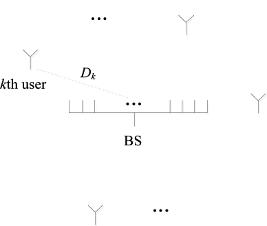
Figure 1: The system model of uplink MU-MIMO system.

In our work, we focus on the uplink MU-MIMO system as shown in Fig. 1, which consists of one BS equipped with $N$ antennas and $K$ single-antenna mobile users. The users transmit their data to the BS in the same time-frequency resource and the $N\times 1$ the received signal column vector at BS equals to

$${\bf{y}}=\sqrt{p_{u}}{\bf{G}}{\bf{x}}+{\bf{w}},$$ (1)

where the $K\times 1$ column vector $\sqrt{p_{u}}{\bf{x}}$ denotes the signal transmitted by the $K$ users. Without loss of generality, the average transmit power of each user is assumed to be $P$. In addition, symbol ${\bf{G}}$ represents the $N\times K$ channel matrix between the BS and the $K$ users and the $\{n,k\}^{\rm{th}}$ entry $g_{nk}\buildrel\Delta\over{=}[{\bf{G}}]_{nk}$ is the channel coefficient between the $n$th antenna at the BS and the $k$th user. The $K\times 1$ column vector ${\bf{w}}$ denotes the additive zero-mean Gaussian white noise with unit variance.

In general, the channel matrix ${\bf{G}}$ is made of two kinds of fading, i.e., fast fading and large-scale fading. Then each element of ${\bf{G}}$ can be written as

$${g_{nk}}={h_{nk}}\sqrt{{\beta_{k}}},n=1,2,\ldots,N,k=1,2,\ldots,K,$$ (2)

where ${h_{nk}}$ is the fast fading coefficient between the $n$th antenna of the BS and the $k$th user. Symbol $\sqrt{{\beta_{k}}}$ denotes the large-scale fading from the $k$th user and the BS, which equals

$${{\beta_{k}}}=\mu_{k}/D_{k}^{v},k=1,2,\ldots,K,$$ (3)

where $D_{k}$ is the distance between the $k$th user to the BS, $v$ is the path-loss exponent with typical values ranging from 2 to 6. The large-scale fading coefficient $\mu_{k}$ is modeled as independent and identically distributed (i.i.d.) gamma random variable (RV), the PDF of which can be expressed as

$$p\left({{\mu_{k}}}\right)=\frac{{{\mu_{k}}^{{m_{k}}-1}}}{{\Gamma\left({{m_{k}}}\right){\Omega_{k}}^{{m_{k}}}}}\exp\left({-\frac{{{\mu_{k}}}}{{{\Omega_{k}}}}}\right),{\mu_{k}},{\Omega_{k}},{m_{k}}>0,$$ (4)

where $\Gamma(\cdot)$ denotes the gamma function. Moreover, denoting $E[\cdot]$ as the expectation of a RV, $m_{k}$ and $\Omega_{k}=E[\mu_{k}]/{m_{k}}$ are the shape and scale parameters of the gamma distribution, respectively. In practical situations it is expected that nonzero small and finite but large values of $m$ for urban and open areas, respectively. The moderate values of $m$ corresponds to suburban and rural areas.

III Ergotic capacity of the uplink MU-MIMO system

In this section, we first derive the expressions of the ergotic capacity of single user in the uplink MU-MIMO system to clarify the relationship between the ergodic capacity and the large-scale fading clearly. Furthermore, the average ergotic capacity of all the users in a cell is also analyzed to describe the network performance. Since in massive MIMO systems zero-forcing (ZF) detector tends to be optimal [4], it is adopted here as the beamformig strategy.

III-A Ergotic capacity of uplink MU-MIMO with perfect CSI

III-A1 Ergotic capacity of the $k$th user

With an ideal assumption that the BS has perfect CSI, the lower bound of the capacity of the $k$th user in this case can be given by [4, Eq. (13)]

$${C_{P,k}^{L}}={\log_{2}}\left({1+{\beta_{k}}{p_{u}}(M-K)}\right).$$ (5)

In the above expression (5), the involved large scale fading parameter ${\beta_{k}}$ is a variable, here we take a further step to analyze the ergodic capacity over ${\beta_{k}}$.

Theorem 1

Considering large-scale fading, the ergodic capacity of the $k$th user with perfect CSI is

$$E\left[{{C_{P,k}^{L}}}\right] =\frac{{\Omega_{k}{{p_{u}}(M-K)}{{m_{k}}}}}{{\ln\left(2\right)D_{k}^{v}}}\ {}_{3}{F_{1}}\left({\begin{array}[]{*{20}{c}}{{m_{k}}+1,1,1}\\ 2\end{array};-\frac{{\Omega_{k}{p_{u}}(M-K)}}{{D_{k}^{v}}}}\right),$$ (8)

where ${}_{p}{F_{q}}\left({\begin{array}[]{*{20}{c}}{{a_{1,}}\ldots,{a_{p}}}\\ {{b_{1}},\ldots,{b_{q}}}\end{array};z}\right)$ is the generalized hypergeometric function.

Proof.

See Appendix A. ∎

III-A2 Average ergotic capacity of all the users

In the considered communication systems, the coverage area of a cell is model as a disc and the BS is located in the center of the cell. The mobile users are located uniformly in the cell with $R_{0}<D_{k}<R$. The distribution of the users along the radius of the cell is expressed as

$$f_{d}\left(x\right)=\frac{{2K}}{{{R^{2}-R_{0}^{2}}}}x.$$ (9)

where $x$ is the distance between one user and the BS.

Exploiting Eqs. (8) and (9), the lower bound of the average capacity of all the users in the cell, noting as $\bar{C}_{P}^{L}$, can be averaged after deriving the integral over the radius as

$$\bar{C}_{P}^{L} =\frac{1}{K}\sum\limits_{k=1}^{K}{E\left[{C_{P,k}^{L}}\right]}$$

$$\mathop{\to}\limits^{a.s.}\frac{2}{{{R^{2}-R_{0}^{2}}}}\int_{{R_{0}}}^{R}{x\frac{{\Omega_{k}{p_{u}}(M-K){{m_{k}}}}}{{\ln\left(2\right){x^{v}}}}\times{\;{}_{3}}{F_{1}}\left({\begin{array}[]{*{20}{c}}{{m_{k}}+1,1,1}\\ 2\end{array};-\frac{{\Omega_{k}{p_{u}}(M-K)}}{{{x^{v}}}}}\right)}dx.$$ (12)

Therefore the integral in the above expression (III-A2) becomes to the concern of the following work.

Theorem 2

Considering the distribution of large-scale fading, the average ergodic capacity of all the users with perfect CSI is

$$\bar{C}_{P}^{L} \mathop{\to}\limits^{a.s.}\frac{{2\Omega_{k}{p_{u}}(M-K){m_{k}}}}{{\ln\left(2\right)\left({{R^{2}}-R_{0}^{2}}\right)\left(v-2\right)}}\Bigg{\{}\frac{1}{{{R_{0}}^{v-2}}}{}_{4}{F_{2}}\left({\begin{array}[]{*{20}{c}}{\frac{{v-2}}{v},{m_{k}}+1,1,1}\\ {\frac{{v-2}}{v}+1,2}\end{array};\frac{{-\Omega_{k}{p_{u}}(M-K)}}{{{R_{0}}^{v}}}}\right)$$ (15)

$$\quad-\frac{1}{{{R^{v-2}}}}{}_{4}{F_{2}}\left({\begin{array}[]{*{20}{c}}{\frac{{v-2}}{v},{m_{k}}+1,1,1}\\ {\frac{{v-2}}{v}+1,2}\end{array};\frac{{-\Omega_{k}{p_{u}}(M-K)}}{{{R^{v}}}}}\right)\Bigg{\}}.$$ (18)

Proof.

See Appendix B. ∎

Perfect CSI is only an ideal assumption. In practice, CSI should be estimated via training sequences or pilots. Due to limited length of training sequences and time varying nature of wireless channels, channel estimation errors are inevitable. In the following section, the performance with imperfect CSI is analyzed.

III-B Ergotic capacity of uplink MU-MIMO with imperfect CSI

In this subsection we take a further step to derive several useful expressions of the ergodic capacity of the massive MIMO systems with imperfect CSI. In practice, the channel matrix $\bf{G}$ need to be estimated with the assistance of pilots [8]. During the training phase in the coherence interval, mutually orthogonal pilot signals of length $\tau$ are transmitted by different users. The pilot sequences used by all the users are denoted as a $\tau\times K$ matrix $\sqrt{\tau p_{u}}{\bf\Phi}$ ($\tau\geq K$) with ${\bf\Phi}^{\rm H}{\bf\Phi}={\bf I}_{K}$. Denoting ${\bf G}$ as the $M\times K$ channel matrix between the BS and the $K$ users, the $M\times\tau$ received pilot matrix at the BS is expressed as

$${\bf Y}_{p}=\sqrt{\tau p_{u}}{\bf G}{\bf\Phi}^{\rm T}+{\bf N},$$ (19)

where ${\bf N}$ is the $M\times\tau$ noise matrix with i.i.d. $CN(0,1)$ elements. The MMSE estimate of ${\bf G}$ is

$${\bf{\hat{G}}}=\frac{1}{{\sqrt{\tau{p_{u}}}}}{{\bf{Y}}_{p}}{\bf{\Phi\tilde{D}}}=\left({{\bf{G}}+\frac{1}{{\sqrt{\tau{p_{u}}}}}{\bf{W}}}\right){\bf{\tilde{D}}},$$ (20)

where ${\bf{W}}\buildrel\Delta\over{=}{\bf N\Phi^{*}}$ has i.i.d. $CN(0,1)$ elements, as ${\bf\Phi}^{\rm H}{\bf\Phi}={\bf I}_{K}$. Since ${\bf{D}}=diag\left\{{{\beta_{i}}}\right\},i\in\left[{1,K}\right]$ denotes the favorable propagation, we have matrix ${\bf{\tilde{D}}}\buildrel\Delta\over{=}{\left({\frac{1}{{\tau{p_{u}}}}{{\bf{D}}^{{\bf{-1}}}}+{{\bf{I}}_{K}}}\right)^{-1}}=diag\left\{{\frac{{\tau{p_{u}}{\beta_{i}}}}{{\tau{p_{u}}{\beta_{i}}+1}}}\right\}$, $i\in\left[{1,K}\right]$. Denoting the channel estimation error as ${{\bf{G}}_{\Delta}}={\bf{\hat{G}}}-{\bf{G}}$, it can be seen that the elements of the $i$th column of ${{\bf{G}}_{\Delta}}$ are RVs with zero means and variances ${\frac{{\tau{p_{u}}{\beta_{i}}}}{{\tau{p_{u}}{\beta_{i}}+1}}}$, which will decrease the received signal to noise ratio (SNR) at the BS.

III-B1 Ergotic capacity of the $k$th user

With imperfect CSI, we begin with the derivation of the ergodic capacity of the $k$th user by employing a lower bound given as [4, Eq. (42)]

$${C_{IP,k}}\geq{\log_{2}}\left({1+\frac{{\tau p_{u}^{2}\left({M-K}\right)\beta_{k}^{2}}}{{\left({\tau p_{u}\beta_{k}+1}\right)\sum\limits_{i=1}^{K}{\frac{{p_{u}\beta_{i}}}{{\tau p_{u}\beta_{i}+1}}}+\tau p_{u}\beta_{k}+1}}}\right).$$ (21)

However, the bound given in [4, Eq. (42)] is complex and not possible to calculate the integral over ${\beta_{k}}$. Using the fact that $\frac{{p_{u}\beta_{i}}}{{\tau p_{u}\beta_{i}+1}}\leq\frac{1}{\tau}$ and $1+\frac{a}{b}\geq\frac{{1+a}}{b},a\geq 0,b\geq 1$, a novel lower bound is proposed as

$${C_{IP,k}}\geq{\log_{2}}\left({1+\tau p_{u}^{2}\left({M-K}\right)\beta_{k}^{2}}\right)-{\log_{2}}\left({1+\tau p_{u}\beta_{k}}\right)-{\log_{2}}\left({1+\frac{K}{\tau}}\right)\buildrel\Delta\over{=}C_{IP,k}^{L}.$$ (22)

Now we derive the integral over the large-scale fading ${\beta_{k}}$ in the above expression (22) and obtain the following theorem.

Theorem 3

Taking the large-scale fading into account, the ergodic capacity of the $k$th user with imperfect CSI is

$$E\left[{C_{IP,k}^{L}}\right]$$

$$=\underbrace{\frac{{\tau\Omega_{k}^{2}p_{u}^{2}\left({M-K}\right){2^{{m_{k}}+1}}\Gamma\left({\frac{{{m_{k}}}}{2}+1}\right)\Gamma\left({\frac{{{m_{k}}}}{2}+\frac{3}{2}}\right)}}{{\sqrt{\pi}\ln\left(2\right)\Gamma\left({{m_{k}}}\right)D_{k}^{2v}}}{\;{}_{4}}{F_{1}}\left({\begin{array}[]{*{20}{c}}{\frac{{{m_{k}}}}{2}+1,\frac{{{m_{k}}}}{2}+\frac{3}{2},1,1}\\ 2\end{array};-\frac{{4\tau\Omega_{k}^{2}p_{u}^{2}\left({M-K}\right)}}{{D_{k}^{2v}}}}\right)}_{{{{\Xi_{\rm{1}}}\left({{D_{k}},{m_{k}},{p_{u}},v}\right)}}}$$ (25)

$$\quad-\underbrace{\frac{{\tau\Omega_{k}{p_{u}}{m_{k}}}}{{\ln\left(2\right)D_{k}^{v}}}{\;{}_{3}}{F_{1}}\left({\begin{array}[]{*{20}{c}}{{m_{k}}+1,1,1}\\ 2\end{array};-\frac{{\tau\Omega_{k}{p_{u}}}}{{D_{k}^{v}}}}\right)}_{{{{\Xi_{\rm{2}}}\left({{D_{k}},{m_{k}},{p_{u}},v}\right)}}}-{\log_{2}}\left({1+\frac{K}{\tau}}\right).$$ (28)

Proof.

See Appendix C. ∎

III-B2 Average ergotic capacity of all the users

With the aid of Theorem 3, we are capable to derive the average ergodic capacity of all the user with imperfect CSI, which can be derived following the same logic of the perfect CSI case as

$$\bar{C}_{IP}^{L}\mathop{\to}\limits^{a.s.}\frac{2}{{{R^{2}}-R_{0}^{2}}}\int_{R_{0}^{2}}^{R}x{\Xi_{\rm{1}}}\left({x,{m_{k}},{p_{u}},v}\right)dx-\frac{2}{{{R^{2}}-R_{0}^{2}}}\int_{R_{0}^{2}}^{R}x{\Xi_{2}}\left({x,{m_{k}},{p_{u}},v}\right)dx-{\log_{2}}\left({1+\frac{K}{\tau}}\right).$$ (29)

Deriving the integral of Eq. (29) yields the following theorem.

Theorem 4

Taking the effects of the large-scale fading into account, the average ergodic capacity of all the users with imperfect CSI is

$${{\bar{C}}_{IP}} \mathop{\to}\limits^{a.s.}\frac{{\tau\Omega_{k}^{2}p_{u}^{2}\left({M-K}\right){2^{{m_{k}}}}\Gamma\left({\frac{{{m_{k}}}}{2}+1}\right)\Gamma\left({\frac{{{m_{k}}}}{2}+\frac{3}{2}}\right)}}{{\left({{R^{2}}-R_{0}^{2}}\right)\sqrt{\pi}\ln\left(2\right)\Gamma\left({{m_{k}}}\right)\left(v-1\right)}}$$

$$\quad\times\Bigg{\{}\frac{1}{{{R_{0}}^{2v-2}}}{}_{5}{F_{2}}\left({\begin{array}[]{*{20}{c}}{\frac{{v-1}}{v},\frac{{{m_{k}}}}{2}+1,\frac{{{m_{k}}}}{2}+\frac{3}{2},1,1}\\ {\frac{{v-1}}{v}+1,2}\end{array};\frac{{-4\tau\Omega_{k}^{2}p_{u}^{2}\left({M-K}\right)}}{{{R_{0}}^{2v}}}}\right)$$ (32)

$$\quad\quad\quad\quad-\frac{1}{{{R^{2v-2}}}}{}_{5}{F_{2}}\left({\begin{array}[]{*{20}{c}}{\frac{{v-1}}{v},\frac{{{m_{k}}}}{2}+1,\frac{{{m_{k}}}}{2}+\frac{3}{2},1,1}\\ {\frac{{v-1}}{v}+1,2}\end{array};\frac{{-4\tau\Omega_{k}^{2}p_{u}^{2}\left({M-K}\right)}}{{{R^{2v}}}}}\right)\Bigg{\}}$$ (35)

$$\quad-\frac{{2\tau\Omega_{k}{p_{u}}{m_{k}}}}{{\ln\left(2\right)\left({{R^{2}}-R_{0}^{2}}\right)\left(v-2\right)}}\Bigg{\{}\frac{1}{{{R_{0}}^{v-2}}}{}_{4}{F_{2}}\left({\begin{array}[]{*{20}{c}}{\frac{{v-2}}{v},{m_{k}}+1,1,1}\\ {\frac{{v-2}}{v}+1,2}\end{array};\frac{{-\tau\Omega_{k}{p_{u}}}}{{{R_{0}}^{v}}}}\right)$$ (38)

$$\quad\quad\quad\quad-\frac{1}{{{R^{v-2}}}}{}_{4}{F_{2}}\left({\begin{array}[]{*{20}{c}}{\frac{{v-2}}{v},{m_{k}}+1,1,1}\\ {\frac{{v-2}}{v}+1,2}\end{array};\frac{{-\tau\Omega_{k}{p_{u}}}}{{{R^{v}}}}}\right)\Bigg{\}}-{\log_{2}}\left({1+\frac{K}{\tau}}\right).$$ (41)

Proof.

Due to space limitations, we will skip the proof, which can be obtained following the similar logics of Appendices B and C. ∎

We note that all the expressions in the theorems of this section are novel and can be used to predict the ergodic capacity of the large uplink MU-MIMO systems over generalized-$K$ fading channels. It is also worth noting that they are closed-form expressions, involving only a finite number of basic operations such as summations of logarithms, Gamma functions, and generalized hypergeometric function, etc. This result can be used to determine the radius of the coverage of massive MIMO base stations.

IV Numerical results

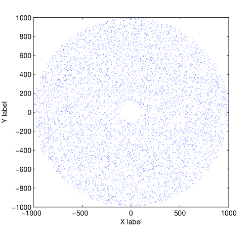
Figure 2: The distribution of the users in the cell.

In this section, simulation results are presented to examine the impact of network parameters on the ergodic capacity of the large uplink MU-MIMO systems. We assume that the users are located uniformly in a cell of $1000$ meters while no user is closer to the BS than $100$ meters, which means that $R=1000$ and $R_{0}=100$. The distribution of the users is plotted in Fig. 2. The transmitted signals suffer from the Nakagami-$m$ distributed fast fading (we set the fast fading parameter $m=1$), and the gamma distributed large-scale fading (we set $\Omega_{k}=1/{m_{k}}$ and $m_{1}=m_{2}=\ldots=m_{K}=m$). We also assume equal transmit power at each node and the value of $P$ is set to be the received power at $500$ meters far from the transmitted users. The length of the pilot is set as $\tau=K$. Furthermore, the path loss exponent is set as $v=3.6$ [9].

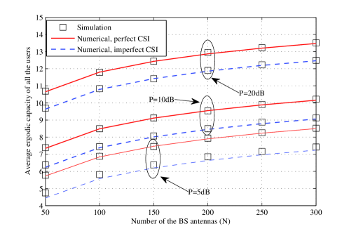
Figure 3: The average ergodic capacity of all the users with different number of BS antennas $N$ in the case of $K=9$, $m=3.3$, and $P=5dB,10dB,20dB$.

Fig. 3 plots both the simulated and numerical average capacity of all the users with different number of the BS antennas $N$. The number of the users is set as $K=9$ and the large-scale fading parameter is set as $m=3.3$. It can be seen that the numerical curves accurately predict the simulated ones in the large number of $N$ with both perfect and imperfect CSI. By observing these curves, it is evident that the capacity increases with $N$, which indicates that increasing the number of the BS antennas brings an improved performance of system throughput. For example, increasing $N$ from $100$ to $300$ brings a capacity advantage of almost $20\%$ at $P=10dB$ with perfect CSI. It is also evident that the lack of CSI will decrease the capacity of the system. For example, the imperfect CSI brings about a capacity loss of $12\%$ at $P=10dB$ with $N=250$.

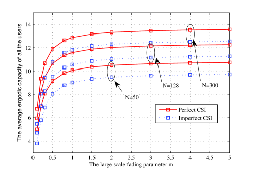
Figure 4: The average ergodic capacity of all the users with different large scale fading parameter $m$ in the case of $K=9$, $N=50,128,300$, and $P=20dB$.

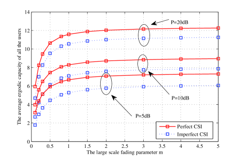
Figure 5: The average ergodic capacity of all the users with different large scale fading parameter $m$ in the case of $K=9$, $N=128$, and $P=5dB,10dB,20dB$.

Figs. 4 and 5 plot the average capacity of all the users with different large-scale fading parameters $m$. We set $K=9$. It can be observed that increasing $m$ will result in a better average capacity of all the users in both figures. For example, increasing $m$ from $0.1$ to $1$ brings about a capacity advantage of $93\%$ at $N=128,P=20dB$ with perfect CSI. Increasing $m$ from $2$ to $5$ brings about a capacity advantage of $2\%$ at $N=128,P=20dB$ with perfect CSI. Similar observations can be obtained by the curves with imperfect CSI. These observations demonstrate that with both perfect CSI and imperfect CSI, the average ergodic capacity of all the users increases obversely as $m$ goes large when $m<2$, which is the urban scenario with heavy shadowing; larger $m$ will brings little improvement of the capacity when $m>2$, which is the suburban, rural, or flatland scenario.

V Conclusions

In this correspondence, we analyzed the ergodic capacity of a large uplink MU-MIMO system where multiple single-antenna users transmit their information to a base station equipped with a very large number of antennas. Over generalized-$K$ fading channels, several novel lower bounds of the ergodic capacity of a single user were derived for both perfect CSI and imperfect CSI, as well as the average ergodic capacity of all the users in the cell. Simulation results were used to validate our analytical expressions. We figured out that large-scale fading will have large effect on the capacity of the system with both perfect and imperfect CSI in the urban scenario. Our result is of importance to design the coverage of massive MIMO base stations.

Appendix A Proof of Theorem 1

Substituting Eqs. (3) and (4) into Eq. (5), the ergodic capacity of the $k$th user can be expressed as

$$E\left[{{C_{P,k}^{L}}}\right]= \int_{0}^{\infty}{{{\log}_{2}}\left({1+\frac{{{p_{u}}(M-K)}}{{D_{k}^{v}}}{\mu_{k}}}\right)}\frac{{{\mu_{k}}^{{m_{k}}-1}}}{{\Gamma\left({{m_{k}}}\right){\Omega_{k}}^{{m_{k}}}}}\exp\left({-\frac{{{\mu_{k}}}}{{{\Omega_{k}}}}}\right)d{\mu_{k}}.$$ (42)

Employing ${\log_{2}}\left(x\right)=\ln\left(x\right)/\ln\left(2\right)$ and $\ln\left({1+x}\right)=\sum\limits_{i=0}^{\infty}{{{\left({-1}\right)}^{i}}{x^{i+1}}/({i+1})}$ [11, 1.511], we can rewrite the above expression (42) as

$$E\left[{C_{P,k}^{L}}\right]=-\frac{1}{{\ln\left(2\right)\Gamma\left({{m_{k}}}\right){\Omega_{k}}^{{m_{k}}}}}\sum\limits_{i=0}^{\infty}{\frac{1}{{i+1}}}{\left({-\frac{{{{{p_{u}}(M-K)}}}}{{D_{k}^{v}}}}\right)^{i+1}}\int_{0}^{\infty}{{\mu_{k}}^{{m_{k}}+i}\exp\left({-\frac{{{\mu_{k}}}}{{{\Omega_{k}}}}}\right)d}{\mu_{k}}.$$ (43)

Using the formula given by [11, 3.326.2], the above expression (43) can be expressed as

$$E\left[{C_{P,k}^{L}}\right] =-\frac{1}{{\ln\left(2\right)\Gamma\left({{m_{k}}}\right)}}\sum\limits_{i=0}^{\infty}{\frac{1}{{i+1}}}\Gamma\left({{m_{k}}+i+1}\right){\left({-\frac{{\Omega_{k}{p_{u}}(M-K)}}{{D_{k}^{v}}}}\right)^{i+1}}.$$ (44)

Multiplying the same items on both the numerators and denominators in the fractions does not change the equality and thus Eq. (44) can be rewritten as

$$E\left[{C_{P,k}^{L}}\right] =\frac{{\Omega_{k}{p_{u}}(M-K)\Gamma\left({{m_{k}}+1}\right)}}{{\ln\left(2\right)\Gamma\left({{m_{k}}}\right)D_{k}^{v}}}\sum\limits_{i=0}^{\infty}{\frac{{\Gamma\left({{m_{k}}+1+i}\right)}}{{\Gamma\left({{m_{k}}+1}\right)}}}\frac{{\Gamma\left({i+1}\right)\Gamma\left({i+1}\right)\Gamma\left(2\right)}}{{\Gamma\left(1\right)\Gamma\left(1\right)\Gamma\left({i+2}\right)}}\frac{{{{\left({-\frac{{\Omega_{k}{p_{u}}(M-K)}}{{D_{k}^{v}}}}\right)}^{i}}}}{{\Gamma\left({i+1}\right)}}$$

$$=\frac{{\Omega_{k}{p_{u}}(M-K)\Gamma\left({{m_{k}}+1}\right)}}{{\ln\left(2\right)\Gamma\left({{m_{k}}}\right)D_{k}^{v}}}\sum\limits_{i=0}^{\infty}{}\frac{{{{\left({{m_{k}}+1}\right)}_{i}}{{\left(1\right)}_{i}}{{\left(1\right)}_{i}}}}{{{{\left(2\right)}_{i}}}}\frac{{{{\left({-\frac{{\Omega_{k}{p_{u}}(M-K)}}{{D_{k}^{v}}}}\right)}^{i}}}}{{i!}},$$ (45)

where ${\left(m\right)_{i}}=\Gamma\left({m+i}\right)/\Gamma\left(m\right)$ is named as the Pochmann symbol. Based on [10, 16.2.1], Eq. (A) can be reformulated as Eq. (8) and then the theorem can be achieved.

Appendix B Proof of Theorem 2

Substituting Eq. (44) into Eq. (III-A2) and using the formula $\int{{x^{a}}}dx={x^{a+1}}/\left({a+1}\right)$, we can reformulate (III-A2) as

$$\bar{C}_{P}^{L} \mathop{\to}\limits^{a.s.}\frac{{{\rm{2}}\Omega_{k}{p_{u}}(M-K)\Gamma\left({{m_{k}}+1}\right)\Gamma\left({\frac{{v-2}}{v}}\right)}}{{v\ln\left(2\right)({R^{2}}-R_{0}^{2})\Gamma\left({{m_{k}}}\right)\Gamma\left({\frac{{v-2}}{v}+1}\right)}}\sum\limits_{i=0}^{\infty}{\frac{{\Gamma\left({i+1}\right)\Gamma\left({i+1}\right)\Gamma\left(2\right)\Gamma\left({i+\frac{{v-2}}{v}}\right)}}{{\Gamma\left(1\right)\Gamma\left(1\right)\Gamma\left({i+2}\right)\Gamma\left({\frac{{v-2}}{v}}\right)}}}$$

$$\quad\times\frac{{\Gamma\left({\frac{{v-2}}{v}+1}\right)\Gamma\left({{m_{k}}+i+1}\right)}}{{\Gamma\left({i+\frac{{v-2}}{v}+1}\right)\Gamma\left({{m_{k}}+1}\right)}}\left({\frac{1}{{{R_{0}}^{v-2}}}\frac{{{{\left({\frac{{-\Omega_{k}{p_{u}}(M-K)}}{{{R_{0}}^{v}}}}\right)}^{i}}}}{{i!}}-\frac{{\rm{1}}}{{{R^{v-2}}}}\frac{{{{\left({\frac{{-\Omega_{k}{p_{u}}(M-K)}}{{{R^{v}}}}}\right)}^{i}}}}{{i!}}}\right).$$ (46)

Based on the definition of Pochmann symbol, the above expression (B) can be expressed as

$$\bar{C}_{P}^{L} \mathop{\to}\limits^{a.s.}\frac{{{\rm{2}}\Omega_{k}{p_{u}}(M-K)\Gamma\left({{m_{k}}+1}\right)\Gamma\left({\frac{{v-2}}{v}}\right)}}{{v\ln\left(2\right)({R^{2}}-R_{0}^{2})\Gamma\left({{m_{k}}}\right)\Gamma\left({\frac{{v-2}}{v}+1}\right)}}$$

$$\quad\times\Bigg{\{}\frac{1}{{{R_{0}}^{v-2}}}\sum\limits_{i=0}^{\infty}{\frac{{{{\left(1\right)}_{i}}{{\left(1\right)}_{i}}{{\left({\frac{{v-2}}{v}}\right)}_{i}}{{\left({{m_{k}}+1}\right)}_{i}}}}{{{{\left(2\right)}_{i}}{{\left({\frac{{v-2}}{v}+1}\right)}_{i}}}}}\frac{{{{\left({\frac{{-\Omega_{k}{p_{u}}(M-K)}}{{{R_{0}}^{v}}}}\right)}^{i}}}}{{i!}}$$

$$\quad\quad\quad\quad-\frac{{\rm{1}}}{{{R^{v-2}}}}\sum\limits_{i=0}^{\infty}{\frac{{{{\left(1\right)}_{i}}{{\left(1\right)}_{i}}{{\left({\frac{{v-2}}{v}}\right)}_{i}}{{\left({{m_{k}}+1}\right)}_{i}}}}{{{{\left(2\right)}_{i}}{{\left({\frac{{v-2}}{v}+1}\right)}_{i}}}}}\frac{{{{\left({\frac{{-\Omega_{k}{p_{u}}(M-K)}}{{{R^{v}}}}}\right)}^{i}}}}{{i!}}\Bigg{\}},$$ (47)

based on which and together with [10, 16.2.1], Eq. (15) is obtained and then proof is ended.

Appendix C Proof of Theorem 3

Following a similar logic as the derivation of Eq. (44), the expectation of first item of Eq. (22) over $\beta_{k}$ can be derived to be

$${{\Xi_{\rm{1}}}\left({{D_{k}},{m_{k}},{p_{u}},v}\right)}$$

$$\buildrel\Delta\over{=}E\left[{{{\log}_{2}}\left({1+\tau p_{u}^{2}\left({M-K}\right)\beta_{k}^{2}}\right)}\right]$$

$$=-\frac{1}{{\ln\left(2\right)\Gamma\left({{m_{k}}}\right){\Omega_{k}}^{{m_{k}}}}}\sum\limits_{i=0}^{\infty}{\frac{1}{{i+1}}}{\left({-\frac{{\tau p_{u}^{2}(M-K)}}{{D_{k}^{2v}}}}\right)^{i+1}}\int_{0}^{\infty}{{\mu_{k}}^{{m_{k}}+2i+1}\exp\left({-\frac{{{\mu_{k}}}}{{{\Omega_{k}}}}}\right)d}{\mu_{k}}$$

$$=\frac{{\tau\Omega_{k}^{2}p_{u}^{2}(M-K)}}{{\ln\left(2\right)\Gamma\left({{m_{k}}}\right)D_{k}^{2v}}}\sum\limits_{i=0}^{\infty}{\frac{1}{{i+1}}}\Gamma\left({{m_{k}}+2i+2}\right){\left({-\frac{{\tau\Omega_{k}^{2}p_{u}^{2}(M-K)}}{{D_{k}^{2v}}}}\right)^{i}},$$ (48)

where the last step is obtained by using [11, 3.326.2]. We apply the expression given by [11, 8.335.1] to derive the integral in (C), which can be written as

$$\Gamma\left({2x}\right)=\frac{{{2^{2x-1}}}}{{\sqrt{\pi}}}\Gamma\left(x\right)\Gamma\left({x+\frac{1}{2}}\right).$$ (49)

Substituting (49) into (C), $I_{1}$ can be reformulated as

$${{\Xi_{\rm{1}}}\left({{D_{k}},{m_{k}},{p_{u}},v}\right)} =\frac{{\tau\Omega_{k}^{2}p_{u}^{2}\left({M-K}\right){2^{{m_{k}}+1}}}}{{\sqrt{\pi}\ln\left(2\right)\Gamma\left({{m_{k}}}\right)D_{k}^{2v}}}\sum\limits_{i=0}^{\infty}{\frac{1}{{i+1}}}\Gamma\left({i+\frac{{{m_{k}}}}{2}+1}\right)$$

$$\quad\times\Gamma\left({i+\frac{{{m_{k}}}}{2}+\frac{3}{2}}\right){\left({-\frac{{4\tau\Omega_{k}^{2}p_{u}^{2}\left({M-K}\right)}}{{D_{k}^{2v}}}}\right)^{i}}.$$ (50)

Multiplying the same items on both the numerators and denominators in the fractions, the equality does not change and Eq. (C) can be further rewritten as

$${{\Xi_{\rm{1}}}\left({{D_{k}},{m_{k}},{p_{u}},v}\right)} =\frac{{\tau\Omega_{k}^{2}p_{u}^{2}\left({M-K}\right){2^{{m_{k}}+1}}\Gamma\left({\frac{{{m_{k}}}}{2}+1}\right)\Gamma\left({\frac{{{m_{k}}}}{2}+\frac{3}{2}}\right)}}{{\sqrt{\pi}\ln\left(2\right)\Gamma\left({{m_{k}}}\right)D_{k}^{2v}}}$$

$$\quad\times\sum\limits_{i=0}^{\infty}{}\frac{{\Gamma\left({i+\frac{{{m_{k}}}}{2}+1}\right)\Gamma\left({i+\frac{{{m_{k}}}}{2}+\frac{3}{2}}\right)\Gamma\left({i+1}\right)\Gamma\left({i+1}\right)}}{{\Gamma\left({\frac{{{m_{k}}}}{2}+1}\right)\Gamma\left({\frac{{{m_{k}}}}{2}+\frac{3}{2}}\right)\Gamma\left(1\right)\Gamma\left(1\right)}}$$

$$\quad\times\frac{{\Gamma\left(2\right)}}{{\Gamma\left({i+2}\right)}}\frac{{{{\left({-\frac{{4\tau\Omega_{k}^{2}p_{u}^{2}\left({M-K}\right)}}{{D_{k}^{2v}}}}\right)}^{i}}}}{{\Gamma\left({i+1}\right)}}$$

$$=\frac{{\tau\Omega_{k}^{2}p_{u}^{2}\left({M-K}\right){2^{{m_{k}}+1}}\Gamma\left({\frac{{{m_{k}}}}{2}+1}\right)\Gamma\left({\frac{{{m_{k}}}}{2}+\frac{3}{2}}\right)}}{{\sqrt{\pi}\ln\left(2\right)\Gamma\left({{m_{k}}}\right)D_{k}^{2v}}}$$

$$\quad\times\sum\limits_{i=0}^{\infty}{}\frac{{{{\left({\frac{{{m_{k}}}}{2}+1}\right)}_{i}}{{\left({\frac{{{m_{k}}}}{2}+\frac{3}{2}}\right)}_{i}}{{\left(1\right)}_{i}}{{\left(1\right)}_{i}}}}{{{{\left(2\right)}_{i}}}}\frac{{{{\left({-\frac{{4\tau\Omega_{k}^{2}p_{u}^{2}\left({M-K}\right)}}{{D_{k}^{2v}}}}\right)}^{i}}}}{{i!}}.$$ (51)

Applying [10, 16.2.1] to Eq. (C), the expectation of first term over large-scale fading can be expressed as ${{\Xi_{\rm{1}}}\left({{D_{k}},{m_{k}},{p_{u}},v}\right)}$ of Eq. (4). Since ${\log_{2}}\left({1+\tau p_{u}\beta_{k}}\right)$ is similar to Eq. (5), the expectation of second term of Eq. (22) over $\beta_{k}$ can be also expressed as ${{\Xi_{\rm{2}}}\left({{D_{k}},{m_{k}},{p_{u}},v}\right)}$ of Eq. (4). Thus the proof is ended.

References

• [1] Y.Β Jing and B.Β Hassibi, β€œDistributed space-time coding in wireless relay networks,” IEEE Trans. Wireless Commun., vol. 5, no. 12, pp. 3524–3536, Dec. 2006.
• [2] S.Β Jin, M.Β R. McKay, C.Β Zhong, and K.-K.Β Wong, β€œErgodic capacity analysis of amplify-and-forward MIMO dual-hop systems,” IEEE Trans. Inform. Theory, vol.Β 56, no.Β 5, pp. 2204–2224, May 2010.
• [3] J.Β Zhang, C.-K.Β Wen, S.Β Jin, X.Β Gao, and K.-K. Wong, β€œOn capacity of large-scale MIMO multiple access channels with distributed sets of correlated antennas,” IEEE J. Sel. Areas Commun., vol.Β 31, no.Β 2, pp. 133–148, Feb. 2013.
• [4] H.Β Q.Β Ngo, E.Β G.Β Larsson, and T.Β L. Marzetta, β€œEnergy and spectral efficiency of very large multiuser MIMO systems,” IEEE Trans. Commun., vol.Β 61, no.Β 4, pp. 1436–1449, Apr. 2013.
• [5] H. CramΓ©r, Random Variables and Probability Distributions.Β Β Β Cambridge University Press, 1970.
• [6] A. Laourine, M. -S. Alouini, S. Affes, and A. StΓ©phenne, β€œOn the capacity of generalized-$K$ fading channels,” IEEE Trans. Wireless Commun., vol.Β 7, no. 7, pp. 2441-2445, Jul. 2008.
• [7] C. Zhong, K.-K. Wong, and S. Jin, β€œCapacity bounds for MIMO Nakagami-$m$ fading channels,” IEEE Trans. Signal Process., vol. 57, no. 9, pp. 3613 C3623, Sep. 2009.
• [8] F.Β Gao, T.Β Cui, and A.Β Nallanathan, β€œOptimal training design for channel estimation in decode-and-forward relay networks with individual and total power constraints,” IEEE Trans. Signal Process., vol.Β 56, no.Β 12, pp. 5937–5949, Dec. 2008.
• [9] D. Tse and P. Viswanath, Fundamentals of Wireless Communication.Β Β Β Cambridge University Press, 2005.
• [10] F. W. Olver, D. W. Lozier, R. F. Boisvert, and C. W. Clark, NIST handbook of mathematical functions.Β Β Β Cambridge University Press New York, NY, USA, 2010.
• [11] I.Β S. Gradshteyn and I.Β M. Ryzhik, Table of Integrals, Series, and Products, 7th ed.Β Β Β Academic Press, New York, 2007.
Refer to caption