PREPRINT VERSION
A Hybrid Neuro–Wavelet Predictor for QoS Control and Stability
C. Napoli, G. Pappalardo, and E. Tramontana
PUBLISHED ON: AI*IA 2013: Advances in Artificial Intelligence

BIBITEX:

@incollection{
year={2013},
isbn={978-3-319-03523-9},
booktitle={AI*IA 2013: Advances in Artificial Intelligence},
volume={8249},
series={Lecture Notes in Computer Science},
editor={Baldoni, Matteo and Baroglio, Cristina and Boella, Guido and Micalizio, Roberto},
doi={10.1007/978-3-319-03524-6_45},
title={A Hybrid Neuro–Wavelet Predictor for QoS Control and Stability},
url={http://dx.doi.org/10.1007/978-3-319-03524-6_45},
publisher={Springer International Publishing},
keywords={Neural networks; wavelet analysis; QoS; adaptive systems},
author={Napoli, Christian and Pappalardo, Giuseppe and Tramontana, Emiliano},
pages={527-538}
}

Published version copyright © 2013 SPRINGER

UPLOADED UNDER SELF-ARCHIVING POLICIES

NO COPYRIGHT INFRINGEMENT INTENDED

Abstract

For distributed systems to properly react to peaks of requests, their adaptation activities would benefit from the estimation of the amount of requests. This paper proposes a solution to produce a short-term forecast based on data characterising user behaviour of online services. We use wavelet analysis, providing compression and denoising on the observed time series of the amount of past user requests; and a recurrent neural network trained with observed data and designed so as to provide well-timed estimations of future requests. The said ensemble has the ability to predict the amount of future user requests with a root mean squared error below 0.06%. Thanks to prediction, advance resource provision can be performed for the duration of a request peak and for just the right amount of resources, hence avoiding over-provisioning and associated costs. Moreover, reliable provision lets users enjoy a level of availability of services unaffected by load variations.

1 Introduction

General public internet usage has become an essential everyday matter, e.g. widespread use of social–networks and mass communication media, public administration, home banking, etc. Moreover, the request for stable and continuous internet services has reached a pressing priority. Generally, the solutions employed by service providers to adapt server-side resources on-the-fly have been based on content adaptation and differentiated service strategies [1, 9, 3, 12, 13]. However, such strategies could over-deteriorate the service during load peaks. Moreover, for ensuring a minimum level of quality (QoS), even when sudden variations on the number of requests arise, a large number of (over-provisioned) resources is often used, hence incurring into relevant costs and wasted resources for a considerable time interval. Some approaches guarantee a minimum QoS level once the connection has been established (i.e. non-adaptive multimedia services) [11, 24], or by using bandwidth adaption algorithms (i.e. adaptive wireless services) [18]. However, such solutions are still liable to an effective loss of QoS for end users, when we consider content quality or availability, and, in the worst case, even denial of services (DoS). As an alternative to deterministic scheduling [17] or genetic algorithms [28], neural networks have been used within the area of a multi-objective optimisation problems. In [2] authors provide dynamic admission control while preserving QoS by using hardware-based Hopefield neural networks [33].

When autoregressive moving average models (ARMA), and related generalisations, are used, the underlying assumption, even for the study forecasting host load [10], makes them inappropriate for predictions in non-linear systems exhibiting high levels of variations. Artificial neural networks have been used in several ways to provide an accurate model of the QoS evolution over time. Linear regression models have been applied with the support of neural networks in [16], however without some proper mechanisms, such as time delays or feedback, it is still not possible to dynamically follow the evolution of the extended time series. Machine learning approaches have also been used [25], however such approaches were not designed for on-the-fly adaptation, and are unable to give advantages with respect to user perceived responsiveness [27]. For the above approaches in which the amount of connection requests is unknown, to avoid overloading the server-side, only load balancing and admission control policies have been used. Still when the amount of requests overcomes the available resources, service usability worsening or denial of service cannot be avoided. On the other hand, when more resources can be dynamically allocated, since the amount of the required resources is unknown in advance, it often results in over-provisioning, with negative effects on management and related cost.

This paper investigates the use of Second Generation Wavelet Analysis and Recurrent Neural Network (RNN) to predict over time the amount of connection requests for a service, by using a hybrid wavelet recurrent neural network (WRNN). Recurrent neural networks have been proven powerful enough to gain advantages from the statistical properties of time series. In our experiments, the proposed WRNN has been used to analyse data for the Page view statistics Wikimedia(TM) project, produced by Domas Mituzas and released under Creative Common License. Wavelet analysis has been used in order to reduce data redundancies so as to obtain a representation that can express their intrinsic structure, while the neural networks have been used to have the complexity of non-linear data correlational perform data prediction. Thereby, a relatively accurate forecast of the connection request time series can be achieved even when load peaks arise. The estimated result is fundamental for a management service that performs resource preallocation on demand. The precision of our estimates allows just the right amount of resources to be used.

The rest of this paper is structured as follows. In section 2 the background on wavelet theory is given. Section 3 describes second generation wavelets and how their properties are useful for the proposed forecast. Section 4 provides the proposed neural network configuration. Section 5 reports on the performed experiments and results. Finally, Section 6 draws our conclusions.

2 The basis of Wavelet Theory

This work builds on wavelets and neural networks to model the main characteristics of user behaviour for an online service. Wavelet decomposition is a powerful analysis tool for physical and dynamic phenomena that reduces the data redundancies and yields a compact representation expressing the intrinsic structure of a phenomenon. In fact, the main advantage when using wavelet decomposition is the ability to pack the energy signature of a signal or a time series, and then to express relevant data as a few non-zero coefficients. This characteristic has been proven very useful to optimise the performances of neural networks [14]. Like sine and cosine for Fourier transforms, a wavelet decomposition uses functions, i.e. wavelets, to express a function as a particular expansion of coefficients in the wavelet domain. Once a mother wavelet has been chosen, it is possible, as explained in the following, to create new wavelets by dilates and shifts of the mother wavelet. Such novel generated wavelets, if chosen with certain criteria, eventually form a Riesz basis of the Hilbert space $L^{2}(\mathbb{R})$ of square integrable functions. Such criteria are at the basis of wavelet theory and come from the concept of multiresolution analysis of a signal, also called multiscale approximation. When a dynamic model can be expressed as a time-dependent signal, i.e. described by a function in $L^{2}(\mathbb{R})$, then it is possible to obtain a multiresolution analysis of such a signal. For the space $L^{2}(\mathbb{R})$ such an approximation consists in an increasing sequence of closed subspaces which approximate, with a greater amount of details, the space $L^{2}(\mathbb{R})$, eventually reaching a complete representation of $L^{2}(\mathbb{R})$ itself. A complete description of multiresolution analysis and the relation with wavelet theory can be found in [20].

One-dimensional decomposition wavelets of order $n$ for a signal $s(t)$ give a new representation of the signal itself in an $n$-dimensional multiresolution domain of coefficients plus a certain residual coarse representation of the signal in time. For any discrete time step $\tau$ then, the corresponding $M$ order wavelet decomposition $\mathbf{W}s(\tau)$ of the signal $s(\tau)$ will be given by the vector

$$\mathbf{W}s(\tau)=\left[d_{1}(\tau),d_{2}(\tau),\ldots,d_{M}(\tau),a_{M}(\tau)\right]~{}~{}~{}~{}\forall~{}\tau\in\{\tau_{1},\tau_{2},\ldots,\tau_{N}\}$$ (1)

where $d_{1}$ is the most detailed multiresolution approximation of the series, and $d_{M}$ the least detailed, and $a_{M}$ is the residual signal. Such coefficients express some intrinsic time-energy feature of a signal, i.e. features of a time series, while removing redundancies, and offering a well suited representation, which, as described in Section 3, we give as inputs for a neural network.

It is now possible to give a more rigorous definition of a wavelet. Let us take into account a multiresolution decomposition of $L^{2}(\mathbb{R})$

$$\varnothing\subset V_{0}\subset\ldots\subset V_{j}\subset V_{j+1}\subset\ldots\subset L^{2}(\mathbb{R})$$

If we call $W_{j}$ the orthogonal complement $V_{j}$, then it is possible to define a wavelet as a function $\psi(x)$ if the set of $\{\psi(x-l)|l\in\mathbb{Z}\}$ is a Riesz basis of $W_{0}$ and also meets the following two constraints:

$$\int_{-\infty}^{+\infty}\psi(x)dx=0$$ (2)

and

$$||\psi(x)||^{2}=\int_{-\infty}^{+\infty}\psi(x)\psi^{*}(x)dx=1$$

If the wavelet is also an element of $V_{0}$ then it exists a sequence $\{g_{k}\}$ such that

$$\psi(x)=2\sum\limits_{k\in\mathbb{Z}}g_{k}\psi(2x-l)$$

then the set of functions $\{\psi_{j,l}|j,l\in\mathbb{Z}\}$ is now a Riesz basis of $L^{2}(\mathbb{R})$. It follows that a wavelet function can be used to define an Hilbert basis, that is a complete system, for the Hilbert space $L^{2}(\mathbb{R})$. In this case, the Hilbert basis is constructed as the family of functions $\{\psi_{j,l}|j,l\in\mathbb{Z}\}$ by means of dilation and translation of a mother wavelet function $\psi$ so that $\psi_{j,l}=\sqrt{2^{j}}\psi(2^{j}x-l)$. Hence, given a function $f\in L^{2}(\mathbb{R})$ it is possible to obtain the following decomposition

$$f(x)=\sum\limits_{j,l\in\mathbb{Z}}\langle f|\psi_{j,l}\rangle=\sum\limits_{j,l\in\mathbb{Z}}d_{j,l}\psi_{j,l}(x)$$ (3)

where $d_{j,l}$ are called wavelet coefficients of the given function $f$ in the wavelet basis given by the inner product of $\psi_{j,l}$. Likewise, a projection on the space $V_{j}$ is given by

$$\mathbb{P}_{j}f(x)=\sum\limits_{i}\langle f|\varphi_{i,j}\rangle\varphi_{i,j}(x)$$

where $\varphi_{i,j}$ are called dual scaling functions. When the basis wavelet functions coincide with their duals the basis is orthogonal. Choosing a wavelet basis for the multiresolution analysis corresponds to selecting the dilation and shift coefficients. In this way, by performing the decomposition we obtain the $\{d_{i}|a_{M}\}$ coefficients sets of (1). From now on we will refer to the described schema as first generation wavelets, whilst Section 3 describes second generation wavelets.

For the present work, we adopted Biorthogonal wavelet decomposition (this wavelet family is described in [20]), for which symmetrical decomposition and exact reconstruction are possible with finite impulse response (FIR) filters [26].

3 Second generation Wavelets with RNNs

A multiresolution analysis like the one described in Section 2 can be realised by conjugate wavelet filter banks that decompose the signal, and act similarly to a low/high pass filter couple [29]. An advanced solution has been devised to obtain the same decomposition using a lifting and updating procedure. This procedure, named second generation wavelet, takes advantage of the properties of multiresolution wavelet analysis starting from a very simple set-up and gradually building up a more complex multiresolution decomposition to have some specific properties. The lifting procedure is made of a space-domain superposition of biorthogonal wavelets developed in [30].

The construction is performed by an iterative procedure called lifting and prediction. Lifting consists of splitting the whole time series $x[\tau]$ into two disjoint subsets $x_{e}[\tau]$ and $x_{o}[\tau]$, for the even and odd positions, respectively; whereas prediction consists of generating a set of coefficients $d[\tau]$ representing the error of extrapolation of time series $x_{o}[\tau]$ from series $x_{e}[\tau]$. Then, an update operation combines the subsets $x_{e}[\tau]$ and $d[\tau]$ in a subset $a[\tau]$ so that

$$\left\{\begin{array}[]{rcl}d[\tau]&=&x_{o}[\tau]-\mathbf{P}x_{e}[\tau]\\ a[\tau]&=&x_{e}[\tau]+\mathbf{U}d[\tau]\end{array}\right.$$ (4)

where $\mathbf{P}$ is the prediction operator, and $\mathbf{U}$ is the update operator. Eventually, one cycle for the above procedure creates a complete set of discrete wavelet transforms (DWT) and the relative coefficients $d[\tau]$ and $a[\tau]$. It follows that

$$\left\{\begin{array}[]{rcl}x_{e}[\tau]&=&a[\tau]-\mathbf{U}d[\tau]\\ x_{o}[\tau]&=&d[\tau]+\mathbf{P}x_{e}[\tau]\end{array}\right.$$ (5)

The said construction yields discrete wavelet filters that preserve only a certain number $N$ of low order polynomials in the time series. Having such low-order polynomials, in turn, makes it possible to apply non-linear predictors without affecting the $a[\tau]$ coefficients, which provide a coarse approximation of the time series itself.

A neural network can be build to perform such a construction, i.e. a neural network would act as an inverse second generation wavelet transform. In [6], a neural network with a rich representation of past outputs like a fully connected recurrent neural network (RNN), known as the Williams-Zipser network or Nonlinear Autoregressive network with eXogenous inputs (NARX) [31], has been proven able to generalise and reproduce the behaviour of $\mathbf{P}$ and $\mathbf{U}$ operators, and to structure itself to behave as an optimal discrete wavelet filter. Moreover, for such a kind of RNNs, when applied to the prediction and modelling of stochastic phenomena, like the considered behaviour of users, which lead to a variable number of access requests in time, real time recurrent learning (RTRL) has been proven to be very effective. A complete description of RTRL algorithm, NARX and RNNs can be found in [32, 15].

RTRL has been used to train the RNN and such a trained RNN achieves the ability to perform lifting stages, hence the matching of the time series dynamics at the corresponding wavelet scale. This construction brings the possibility to match non-polynomial and nonlinear signal structures in an optimised straightforward N-dimension means square problem [21]. NARX networks have been proven able to use the intrinsic features of time series in order to predict the following values of the series [23]. One of a class of transfer functions for the RNN has to be chosen to approximate the input-output behaviour in the most appropriate manner. For phenomena having a deterministic dynamic behaviour, the relative time series at a given time point can be modelled as a functional of a certain amount of previous time steps. In such cases, the used model should have some internal memory to store and update context information [19]. This is achieved by feeding the RNN with a delayed version of past data, commonly referred as time delayed inputs [8].

4 Proposed setup for WRNN predictor

As stated in Section 3, it would be desired to have a neural network able to perform the wavelet transform as in a recursive lifting procedure. For this, we could use a mother wavelet as transfer function, however mother wavelets lack of some elementary properties needed by a proper transfer function, such as e.g. the absence of local minima and a sufficient graded and scaled response [14]. This leads us to look for a close enough substitute to approximate the properties of a mother wavelet without affecting the functionalities of the network itself. The function classes that more closely approximate a mother waveform have to be found among the Radial Basis Functions (RBFs) that are good enough as transfer functions and partially approximate half of a mother waveform. It is indeed possible to properly scale and shift a couple of RBFs to obtain a mother wavelet. If we define an RBF function as an $f:[-1,1]\rightarrow\mathbb{R}$ then we could dilate and scale it to obtain a new function

$$\tilde{f}(x+2l)=\left\{\begin{array}[]{rcl}+f(2x+1)&{}{}\hfil&x\in[-1,0)\\ -f(2x-1)&{}{}\hfil&x\in(0,+1]\end{array}\right.~{}~{}~{}~{}\forall~{}l\in\mathbb{Z}$$ (6)

With such a definition, starting from the properties of the RBF, it is then possible to verify the following

$$\int_{2h+1}^{2k+1}\tilde{f}(x)dx=0~{}~{}~{}~{}\forall~{}(h,k)\in\mathbb{Z}^{2}:h<k$$ (7)

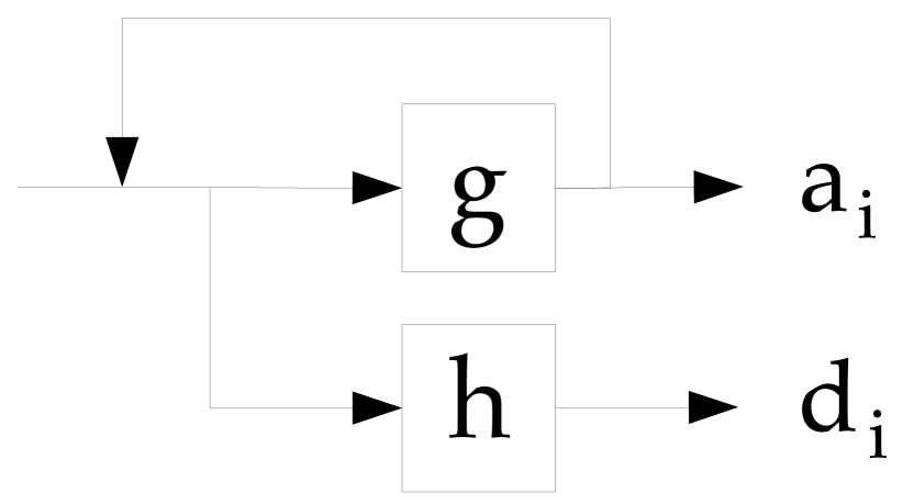
Figure 1: Filter logic

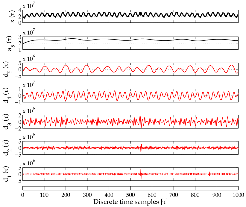
Figure 2: 5-level biorthogonal 3.7 wavelet decomposition

Starting from (6) and (7) it is possible to verify the equations (2) to (3) for the chosen $\tilde{f}$ which we can now call a mother wavelet. The chosen mother wavelet is a composition of two RBF transfer functions that are realised by the proposed neural network to obtain the properties of a wavelet transform. The proposed WRNN has two hidden layers with RBF transfer function.

For this work, the initial dataset was a time series representing access requests coming from users. We call this series $x(\tau)$, where $\tau$ is the discrete time step of the data, sampled with intervals of one hour. A biorthogonal wavelet decomposition of the time series has been computed to obtain the correct input set for the WRNN as required by the devised architecture. This decomposition has been achieved by applying the wavelet transform as a recursive couple of conjugate filters (Figure 2) in such a way that the $i$-esime recursion $\hat{W}_{i}$ produces, for any time step of the series, a set of coefficients $d_{i}$ and residuals $a_{i}$, and so that

$$\hat{W}_{i}[a_{i-1}(\tau)]=[d_{i}(\tau),a_{i}(\tau)]~{}~{}~{}~{}~{}\forall~{}i\in[1,M]\cap\mathbb{N}$$ (8)

where we intend $a_{0}(\tau)=x(\tau)$. The input set can then be represented as an $N\times(M+1)$ matrix of $N$ time steps of a $M$ level wavelet decomposition (see Figure 2), where the $\tau$-esime row represents the $\tau$-esime time step as the decomposition

$$\mathbf{u}(\tau)=\left[d_{1}(\tau),d_{2}(\tau),\ldots,d_{M}(\tau),a_{M}(\tau)\right]$$ (9)

Each row of this dataset is given as input value to the $M$ input neurons of the proposed WRNN. The properties of this network make it possible, starting from an input at a time step $\tau_{n}$, to predict the effective number of access requests at a time step $\tau_{n+r}$. In this way the WRNN acts like a functional

$$\hat{N}[\mathbf{u}(\tau_{n})]=x(\tau_{n+r})$$ (10)

where $r$ is the number of time steps of forecast in the future.

Figure 3: Devised neural netwok

5 Experimental setup

For this work, a 4-level wavelet decomposition has been selected that properly characterises data under analysis. Therefore, the devised WRNN (Figure 3) uses a 5 neuron input layer (one for each level detail coefficient $d_{i}$ and one for the residual $a_{5}$). This WRNN architecture presents two hidden layers with sixteen neurons each and realises a radial basis function as explained in Section 4.

Inputs are given to the WRNN in the following form:

• The wavelet decomposition of the time series $\mathbf{u}(\tau_{n})$ for time step $\tau_{n}$

• The previous delayed decompositions $\mathbf{u}(\tau_{n-1})$ and $\mathbf{u}(\tau_{n-2})$

• The last four delayed outputs $x(\tau_{n+r})$ predicted by the WRNN

Delays and feedback are obtained by using the relative delay lines and operators (D). These feedback lines provide the WRNN with internal memory, hence the modelling abilities for dynamic phenomena.

An accurate study has shown that the biorthogonal wavelet decomposition optimally approximates and denoises the time series under analysis. Such a wavelet family is in good agreement with previous optimal results, obtained by the authors, for the decomposition of other physical phenomena. In fact, such a decomposition splits a phenomenon in a superposition of mutual and concurrent predominant processes with a characteristic time-energy signature. For stochastically-driven processes, such as stellar oscillations [7], renewable energy and systems load [5, 4], and for a large category of complex systems [22], wavelet decomposition gives a unique and compact representation of the leading features for a time-variant phenomenon.

For the case study proposed in this paper we have used the raw data of connection requests over time to predict the behaviour of the users of a widely used an internet service, i.e. the one provided by Wikimedia(TM). Raw data were taken from the page-view statistics Wikimedia(TM) project and released by Domas Mituzas under Creative Common License. Original data report the amount of accesses and bytes for the replies that were sampled in time-steps of one hour for each web page accessible in the project. Data were collected for the whole services offered by Wikimedia projects including Wikipedia(r), Wikidictionary(r), Wikibooks(r) and others. Data were gathered and composed by an automatic procedure, obtaining the total requests made to the wikimedia servers for each hour. Therefore, a 2-years long dataset of hourly sampled access requests has been reconstructed. Then, this dataset was decomposed by using a wavelet biorthogonal decomposition identified by the couple of numbers 3.7, which means that are implemented by using FIR filters with 7th order polynomials degree for the decomposition (see also Figure 5 and 5) and 3rd order for the reconstruction. Decomposed data, as shown in Figure 2, were then given as inputs for the neural network as described in Section 4. The network was trained by using a gradient descent back-propagation algorithm with momentum led adaptive learning rate as presented in [15].

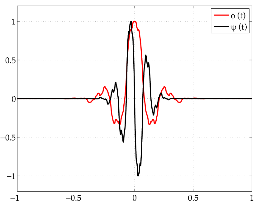
Figure 4: Biorthogonal wavelet 3.7 decomposition ($\psi$) and scaling ($\phi$) functions

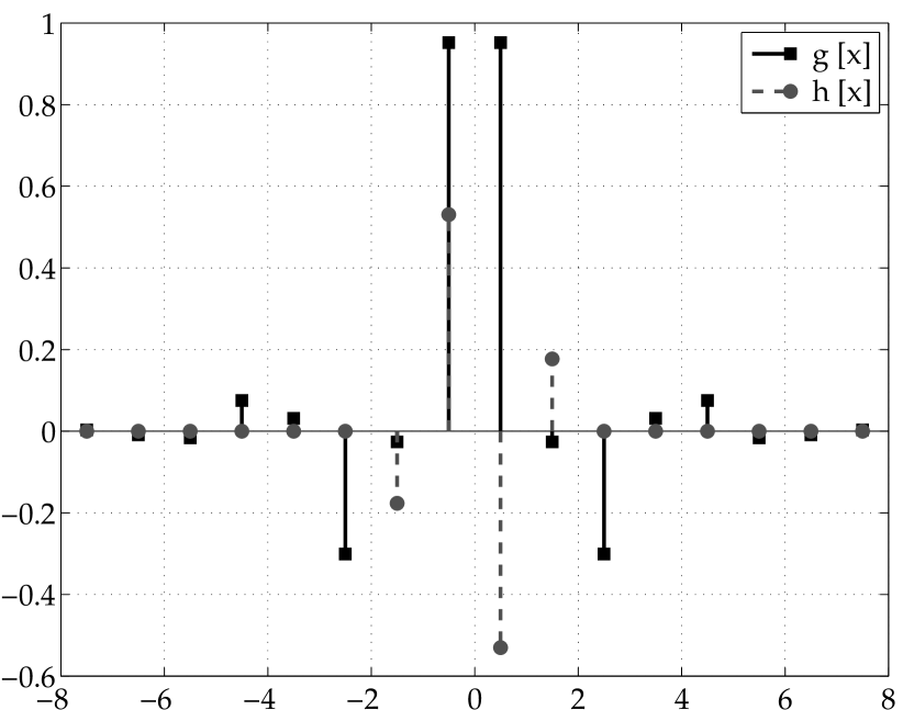
Figure 5: Biorthogonal wavelet 3.7 high-pass (h) and low-pass (g) filers

For a prediction 6 hours in advance of the time series of the amount of requests, the root mean squared error of prediction for the access requests over time was of $1.3156\cdot 10^{04}$ requests, which means a relative error of less than $0.6$ per thousands (less than six requests over ten thousands). Figure 7 shows the shape of the mean square error while training is being performed. Figure 7 shows the actual time series of the incoming requests in black, and the predicted values for the incoming requests in red for a time period of 500 hours. The actual values for the shown time period had not been given as input to the neural network for training, however have then been used to compare with the predicted values and to compute the error (see the bottom part of Figure 7). A smaller period of time has been shown in Figure 8 to highlight the differences of actual and predicted values. As can be seen, the neural network manages to closely predict even relatively small variations of the trends. The output of the neural network was then given to a resource management service to perform allocation requests in terms of needed bandwidth and virtual machines [12].

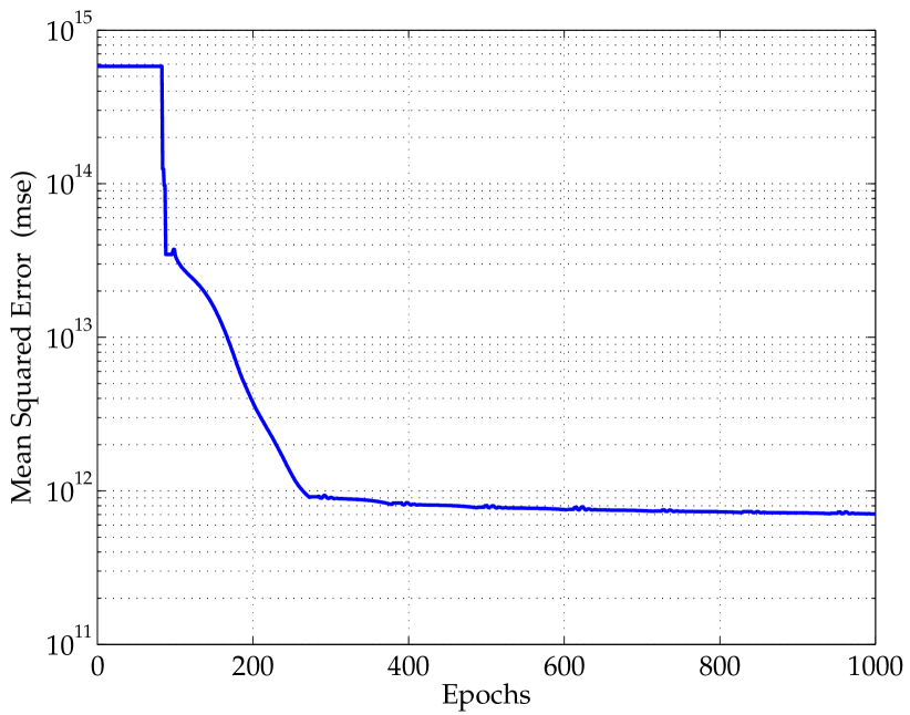
Figure 6: Error while training the network

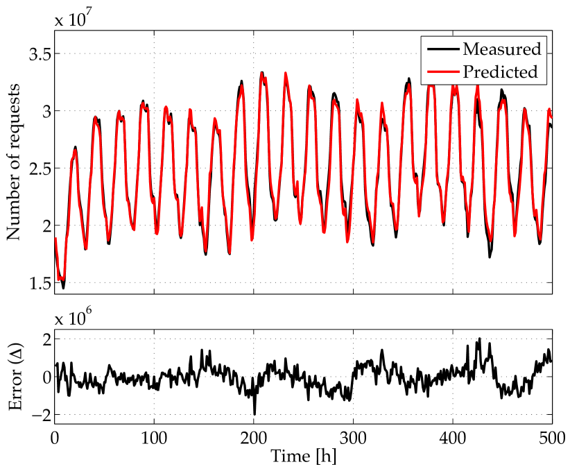
Figure 7: Actual time series and predicted values

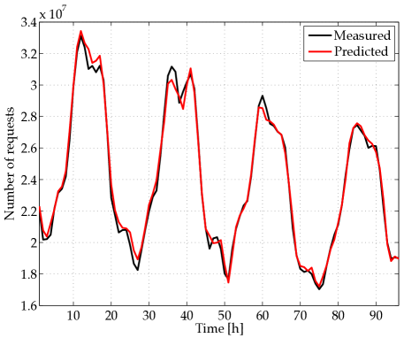
Figure 8: Top of the curves for actual time series and predicted values, for an arbitrary chosen time-interval

6 Conclusions

This paper has provided an ad-hoc architecture for a neural network that is able to predict the amount of incoming requests performed by users when accessing a website. Firstly, the past time series of accesses has been analysed by means of wavelets, which appropriately retain only the fundamental properties of the series. Then, the neural network embeds both the ability to perform wavelet analysis and prediction of future amount of requests. The performed experiments have proven that the provided ensemble is very effective for the desired prediction, since the computed error can be considered negligible.

Estimates can be fundamental for a resource management component, on a server side of an internet based system, since they make it possible to acquire just the right amount of resource (e.g. from a cloud). Then, in turn it is possible to avoid an unnecessary cost and waste of resources, whilst keeping the level of QoS as desired and unaffected by variations of requests.

7 Acknowledgments

This work has been supported by project PRISMA PON04a2 A/F funded by the Italian Ministry of University within PON 2007-2013 framework.

References

- [1] T. F. Abdelzaher, K. G. Shin, and N. Bhatti. Performance guarantees for web server end-systems: A control-theoretical approach. IEEE Transactions on Parallel and Distributed Systems, 13:80–96, 2002.
- [2] C. W. Ahn and R. Ramakrishna. Qos provisioning dynamic connection-admission control for multimedia wireless networks using a hopfield neural network. Transactions on Vehicular Technology, 53(1):106–117, 2004.
- [3] F. Bannò, D. Marletta, G. Pappalardo, and E. Tramontana. Tackling consistency issues for runtime updating distributed systems. In Proceedings of International Symposium on Parallel & Distributed Processing, Workshops and Phd Forum (IPDPSW), pages 1–8. IEEE, 2010. DOI: 10.1109/IPDPSW.2010.5470863.
- [4] F. Bonanno, G. Capizzi, A. Gagliano, and C. Napoli. Optimal management of various renewable energy sources by a new forecasting method. In Proceedings of International Symposium on Power Electronics, Electrical Drives, Automation and Motion (SPEEDAM), pages 934–940. IEEE, 2012.
- [5] G. Capizzi, F. Bonanno, and C. Napoli. A wavelet based prediction of wind and solar energy for long-term simulation of integrated generation systems. In Proceedings of International Symposium on Power Electronics Electrical Drives Automation and Motion (SPEEDAM), pages 586–592. IEEE, 2010.
- [6] G. Capizzi, C. Napoli, and F. Bonanno. Innovative second-generation wavelets construction with recurrent neural networks for solar radiation forecasting. Transactions on Neural Networks and Learning Systems, 23(11):1805–1815, 2012.
- [7] G. Capizzi, C. Napoli, and L. Paternò. An innovative hybrid neuro-wavelet method for reconstruction of missing data in astronomical photometric surveys. In Proceedings of Artificial Intelligence and Soft Computing, pages 21–29. Springer, 2012.
- [8] J. T. Connor, R. D. Martin, and L. Atlas. Recurrent neural networks and robust time series prediction. Transactions on Neural Networks, 5(2):240–254, 1994.
- [9] A. Di Stefano, M. Fargetta, G. Pappalardo, and E. Tramontana. Supporting resource reservation and allocation for unaware applications in grid systems. Concurrency and Computation: Practice and Experience, 18(8):851–863, 2006. DOI: 10.1002/cpe.980.
- [10] P. A. Dinda and D. R. O’Hallaron. Host load prediction using linear models. Cluster Computing, 3(4):265–280, 2000.
- [11] B. Epstein and M. Schwartz. Reservation strategies for multi-media traffic in a wireless environment. In Proceedings of Vehicular Technology Conference, volume 1, pages 165–169. IEEE, 1995.
- [12] R. Giunta, F. Messina, G. Pappalardo, and E. Tramontana. Providing qos strategies and cloud-integration to web servers by means of aspects. Concurrency and Computation: Practice and Experience, 2013. DOI:10.1002/cpe.3031.
- [13] R. Giunta, F. Messina, G. Pappalardo, and E. Tramontana. Kaqudai: a dependable web infrastructure made out of existing components. In Proceedings of Workshops on Enabling Technologies: Infrastructure for Collaborative Enterprises (WETICE). IEEE, 2013. DOI:10.1109/WETICE.2013.47.
- [14] M. M. Gupta, L. Jin, and N. Homma. Static and dynamic neural networks: from fundamentals to advanced theory. Wiley-IEEE Press, 2004.
- [15] S. Haykin. Neural networks and learning machines, volume 3. Prentice Hall New York, 2009.
- [16] S. Islam, J. Keung, K. Lee, and A. Liu. Empirical prediction models for adaptive resource provisioning in the cloud. Future Generation Computer Systems, 28(1):155–162, 2012.
- [17] C. G. Kang, Y. J. Kim, and M. J. Hwang. Implicit scheduling algorithm for dynamic slot assignment in wireless atm networks. Electronics Letters, 34(24):2309–2311, 1998.
- [18] T. Kwon, I. Park, Y. Choi, and S. Das. Bandwidth adaption algorithms with multi-objectives for adaptive multimedia services in wireless/mobile networks. In Proceedings of International Workshop on Wireless Mobile Multimedia, pages 51–59. ACM, 1999.
- [19] A. Lapedes and R. Farber. A self-optimizing, nonsymmetrical neural net for content addressable memory and pattern recognition. Physica D: Nonlinear Phenomena, 22(1):247–259, 1986.
- [20] S. Mallat. A wavelet tour of signal processing: the sparse way. Academic press, 2009.
- [21] D. P. Mandic and J. Chambers. Recurrent neural networks for prediction: Learning algorithms, architectures and stability. John Wiley & Sons, Inc., 2001.
- [22] C. Napoli, F. Bonanno, and G. Capizzi. Exploiting solar wind time series correlation with magnetospheric response by using an hybrid neuro-wavelet approach. In Advances in Plasma Astrophysics, number S274 in Proceedings of the International Astronomical Union, pages 250–252. Cambridge University Press, 2010.
- [23] C. Napoli, F. Bonanno, and G. Capizzi. An hybrid neuro-wavelet approach for long-term prediction of solar wind. In Advances in Plasma Astrophysics, number S274 in Proceedings of the International Astronomical Union, pages 247–249. Cambridge University Press, 2010.
- [24] G. Novelli, G. Pappalardo, C. Santoro, and E. Tramontana. A grid-based infrastructure to support multimedia content distribution. In Proceedings of the workshop on Use of P2P, GRID and agents for the development of content networks (UPGRADE-CN), pages 57–64. ACM, 2007. DOI: 10.1145/1272980.1272983.
- [25] R. Powers, M. Goldszmidt, and I. Cohen. Short term performance forecasting in enterprise systems. In Proceedings of the eleventh ACM SIGKDD international conference on Knowledge discovery in data mining, pages 801–807. ACM, 2005.
- [26] L. R. Rabiner and B. Gold. Theory and application of digital signal processing. Englewood Cliffs, NJ, Prentice-Hall, Inc., 1975. 777 p., 1, 1975.
- [27] S. Schechter, M. Krishnan, and M. D. Smith. Using path profiles to predict http requests. Computer Networks and ISDN Systems, 30(1):457–467, 1998.
- [28] M. R. Sherif, I. W. Habib, M. Nagshineh, and P. Kermani. Adaptive allocation of resources and call admission control for wireless atm using genetic algorithms. Journal on Selected Areas in Communications, 18(2):268–282, 2000.
- [29] W. Sweldens. Lifting scheme: a new philosophy in biorthogonal wavelet constructions. In Proceedings of Symposium on Optical Science, Engineering, and Instrumentation, pages 68–79. International Society for Optics and Photonics, 1995.
- [30] W. Sweldens. The lifting scheme: A construction of second generation wavelets. Journal on Mathematical Analysis, 29(2):511–546, 1998.
- [31] R. J. Williams. A learning algorithm for continually running fully recurrent necurren neural networks. Neural Computation, 1:270–280, 1989.
- [32] R. J. Williams and D. Zipser. Experimental analysis of the real-time recurrent learning algorithm. Connection Science, 1(1):87–111, 1989.
- [33] M. H. Zadeh and M. A. Seyyedi. Qos monitoring for web services by time series forecasting. In Proceedings of International Conference on Computer Science and Information Technology (ICCSIT), volume 5, pages 659–663. IEEE, 2010.