Non-oscillatory flux correlation functions for efficient nonadiabatic rate theory

Abstract

There is currently much interest in the development of improved trajectory-based methods for the simulation of nonadiabatic processes in complex systems. An important goal for such methods is the accurate calculation of the rate constant over a wide range of electronic coupling strengths and it is often the nonadiabatic, weak-coupling limit, which being far from the Born-Oppenheimer regime, provides the greatest challenge to current methods. We show that in this limit there is an inherent sign problem impeding further development which originates from the use of the usual quantum flux correlation functions, which can be very oscillatory at short times. From linear response theory, we derive a modified flux correlation function for the calculation of nonadiabatic reaction rates, which still rigorously gives the correct result in the long-time limit regardless of electronic coupling strength, but unlike the usual formalism is not oscillatory in the weak-coupling regime. In particular, a trajectory simulation of the modified correlation function is naturally initialized in a region localized about the crossing of the potential energy surfaces. In the weak-coupling limit, a simple link can be found between the dynamics initialized from this transition-state region and an generalized quantum golden-rule transition-state theory, which is equivalent to Marcus theory in the classical harmonic limit. This new correlation function formalism thus provides a platform on which a wide variety of dynamical simulation methods can be built aiding the development of accurate nonadiabatic rate theories applicable to complex systems.

I Introduction

The simulation of electronically nonadiabatic dynamics in complex molecular systems poses a significant challenge to current techniques in theoretical chemistry. Tully (2012) These dynamics describe the motion of nuclei in systems in which the Born-Oppenheimer approximation is not valid. This could occur for instance at a conical intersection between two electronic states, Domcke, Yarkony, and Köppel (2004); Levine and Martínez (2007) or as we consider here, near an avoided crossing. [Foranoverview; seeforinstance][andreferencestherein.]Stock2005nonadiabatic In the latter case, the nonadiabatic limit is of special interest, in which the electronic coupling, here referred to as $\Delta$, is weak.

A wide variety of methods have been proposed for performing nonadiabatic dynamics either numerically exactly or with varying degrees of approximation. Stock and Thoss (2005) However, the only systems amenable to exact calculations have either very few degrees of freedom or are model Hamiltonians such as the spin-boson model of electron transfer in the condensed phase, which is defined as a two-level system coupled linearly to a bath of harmonic oscillators. Garg, Onuchic, and Ambegaokar (1985); *Leggett1987spinboson Although an exact closed-form expression for the rate constant of this system is not known, approximate expressions have been formulated by assuming the separability of a reaction coordinate which bridge the various regimes, Rips and Pollak (1995) and otherwise difficult numerical calculations can be made practical by exploiting its simple harmonic form. Weiss (2008)

The treatment of discrete electronic states is naturally described by exact quantum dynamical methods, which differ very little from their Born-Oppenheimer equivalents. Such methods, which have been applied for instance to the spin-boson model, include hybrid approaches which split the system into a small quantum core and large classical reservoir, Wang, Thoss, and Miller (2001); *Thoss2001hybrid and the multilayer multiconfigurational time-dependent Hartree (MCTDH) method, Wang and Thoss (2003); *Thoss2006MLMCTDH; Wang, Skinner, and Thoss (2006) which treats all degrees of freedom quantum mechanically. It is also possible to utilize real-time path-integral approaches Mak and Chandler (1991); Topaler and Makri (1996); Mühlbacher and Egger (2003); *Muehlbacher2004asymmetric to compute the dynamics of system-bath models, where the influence of the harmonic bath can be formally integrated out analytically.

It is not always necessary to calculate the time evolution of the system explicitly in order to obtain the nonadiabatic rate constant. An important example is the golden-rule approach *[Seeforinstance][foraclearderivation.]Zwanzig which employs an approximation valid only in the $\Delta\rightarrow 0$ limit and gives a rate proportional to $\Delta^{2}$. The standard formula, given in Eq. (21), relies on the complete solution of reactant and product states and is thus not directly applicable to complex systems, by which we mean systems for which this set of states are not computable. Application to systems of interest is only possible after an approximation is made that the potential energy surfaces are harmonic with normal modes independent of electronic state. Lee, Dunietz, and Geva (2013) A quantum golden-rule formula has been derived in the case of the spin-boson model, Weiss (2008) which can be written in closed form only after applying an approximate stationary-phase integral. Bader, Kuharski, and Chandler (1990) The celebrated theory of Marcus Marcus (1956) for the rate of electron transfer in the condensed phase *[Seeforinstance][]ChandlerET can be derived from this result in the classical limit and is therefore also known as the classical golden-rule rate. One of the most significant predictions of the theory was the “inverted regime”, in which the rate of electron transfer in strongly exothermic systems decreases with increasing exothermicity, and which was later confirmed by experiment.Miller, Calcaterra, and Closs (1984) We note that the Marcus theory rate is exact in the golden-rule limit for a spin-boson system with classical nuclei, i.e. with heavy masses, and thus provides a benchmark against which nonadiabatic dynamical methods can be tested in this limit.

For complex systems, a procedure commonly followed is to write the golden-rule rate as a time-correlation function of the energy gap between the diabatic states. This is then approximately computed using classical trajectories which evolve on a single surface given by an interpolated average of the diabatic potentials and should thus not be considered as a simulation of the true dynamics but rather as a sampling procedure for estimating the rate constant. The results are not unique due to a dependence of the choice of propagating Hamiltonian and an associated quantum correction factor. Egorov, Rabani, and Berne (1999); Shi and Geva (2004)

A generalization of the golden-rule approach to compute the rate approximately using statistical mechanics, instead of explicitly solving for the states or performing time-propagations, was proposed by Wolynes Wolynes (1987) using a semiclassical approximation to an analytic continuation of the flux-flux correlation function. This gave a nonadiabatic free-energy approach which can be computed numerically using imaginary-time path integral Monte Carlo and is therefore applicable to complex systems. The formalism was rederived by Cao and Voth Cao and Voth (1997) from a nonadiabatic generalization of the $\operatorname{Im}F$ method Coleman (1977); *Affleck1981ImF and has been employed in a number of studies of electron transfer in the condensed phase. Zheng, McCammon, and Wolynes (1989); *Zheng1991ET; Bader, Kuharski, and Chandler (1990); *Marchi1991tunnelling The method requires locating a stationary point of the free energy as a function of imaginary time $\beta^{\prime}\hbar$ about which a steepest-descent imaginary-time integration is performed. There would however be a problem with this approach in the Marcus inverted regime where the stationary point falls outside the interval $[0,\beta\hbar]$ and thus has no meaning for path integrals of period $\beta\hbar$. We also note that due to the steepest-descent time integration, the result is not in general exactly equal to the quantum golden-rule rate, although it may be a good approximation in many cases outside the inverted regime.

A nonadiabatic theory based on imaginary-time path-integral sampling has also been formulatedSchwieters and Voth (1999) which attempts to give the rate constant over the whole range of the electronic coupling $\Delta$. However, in order to ensure the correct $\Delta^{2}$ behaviour in the golden-rule limit, an ad hoc modification of the barrier height was made. The method is not valid for biased systems, and even in the classical limit, does not strictly reduce to the Marcus theory rate for a symmetric system.

In this work, we present an alternative formulation of the golden-rule rate in terms of statistical mechanical quantities which differs from previous approaches and may be a good starting point for the development of a new path-integral golden-rule method applicable to complex systems. We show that the new formulation reduces to the Marcus theory rate constant in the classical limit even in the strongly biased inverted regime. We argue that it is a type of transition-state theory (TST) and show how it is related to dynamical methods.

We now turn to approximate dynamical methods based on nonadiabatic trajectory simulations, which are intended to be interpreted as real-time dynamics. An approximate nonadiabatic rate constant can formally be defined in terms of correlation functions computed using the dynamics. Miller, Schwartz, and Tromp (1983) Such approaches are naturally applicable to complex systems, but an accurate description of the coupling between nuclear and electronic degrees of freedom causes a significant challenge to theory. Stock and Thoss (2005)

The difficulty posed for simulation of nonadiabatic dynamics can be clearly understood by contrasting with the conceptually straightforward case of adiabatic dynamics on a single Born-Oppenheimer surface. In this case, classical Newtonian dynamics are derived from a rigorous heavy-mass limit of quantum mechanics allowing the system to be treated by a molecular dynamics trajectory simulation, which is far less computationally demanding than approaches based on nuclear wave functions and also has the advantage that it can be combined with an on-the-fly calculation of the potential. Due to the inherently quantum nature of the discrete electronic states, no such classical limit exists for nonadiabatic dynamics even in this deceptively simple heavy-mass limit.

The most commonly employed trajectory method is the surface hopping approach of Tully Tully (1990) in which nuclei evolve classically on one of the adiabatic potential energy surfaces with hops between states performed randomly according to a particular algorithm. Many forms exist to determine when the hops should take place and to deal with the energy conservation problem that arises upon instantaneously changing the potential energy of the system. A significant failure of the standard implementation Tully (1990) in the context of this work is that rates do not obey the correct $\Delta^{2}$ dependence in the golden-rule limit. Landry and Subotnik (2011); *Landry2012hopping However, the method is simple to perform and to couple with on-the-fly electronic-structure calculations such that it has gained a high popularity.

An alternative approach for describing electronic-nuclear coupling employs an exact mapping of the Hamiltonian from discrete electronic states to continuous degrees of freedom. Meyer and Miller (1979); Stock and Thoss (1997); *Thoss1999mapping Approximations have been taken to treat the nonadiabatic dynamics from the resulting Hamiltonian classically, Müller and Stock (1998); *Mueller1999pyrazine semiclassically, Stock and Thoss (1997); *Thoss1999mapping; Sun and Miller (1997); Bonella and Coker (2003); Miller (2009) using the linearized semiclassical approach, Sun, Wang, and Miller (1998); Wang et al. (1999) or with centroid-molecular dynamics. Liao and Voth (2002) Recently other methods based on the mapping approach have appeared for treating thermal initial states, Ananth and Miller (2010) using a ring-polymer molecular dynamics (RPMD) Hamiltonian, Richardson and Thoss (2013); Ananth (2013) or in combination with partially linearized real-time path integrals.Huo, Miller III, and Coker (2013)

Other dynamical approaches employ mean-field approximations, Micha (1983) multiple spawning, Ben-Nun and Martínez (2002) the quantum-classical Liouville equation Kapral (2006) or an exact factorization of the complete molecular Hamiltonian. Agostini et al. (2013) Approximate methods intended solely for the estimation of nonadiabatic rate constants include those which treat the transferred electron explicitly with RPMD, Menzeleev, Ananth, and Miller (2011); Kretchmer and Miller III (2013); Shushkov (2013) or use a modified RPMD Hamiltonian to enforce the correct $\Delta^{2}$ dependence in the golden-rule limit. Menzeleev, Bell, and Miller III (2014)

It is a major goal to formulate a nonadiabatic theory which is able to compute the rate constant over a wide range of coupling strengths, $\Delta$, for complex systems. It is obvious that in the adiabatic limit, where the Born-Oppenheimer approximation is valid, such a theory should reduce to something equivalent to classical rate theory, classical TST or ring-polymer TST, Craig and Manolopoulos (2005); Richardson and Althorpe (2009) which is known to be exact in the absence of recrossing. Hele and Althorpe (2013a); *Althorpe2013QTST; Hele and Althorpe (2013b) In this limit, nonadiabatic dynamical approaches Richardson and Thoss (2013); Ananth (2013) can be applied to compute the small amount of dividing-surface recrossing due to nonadiabatic effects. However, this approach breaks down in the weak-coupling limit where the transmission coefficient is extremely small and therefore inefficient to calculate. A quite different form of rate theory is required in this limit which we discuss in this work.

First we outline a general derivation of the rate constant from linear response theory in Sec. II. We then explain the oscillatory problem in the nonadiabatic limit in Sec. III and suggest a solution based on linear response in Sec. IV. We analyse the short-time limit of our approach and hence its relation to dynamical methods in Sec. V. This also leads to a new golden-rule TST formulation described in Sec. VI.1 and we show that its classical limit gives the Marcus theory rate in Sec. VI.2. Finally we summarize our findings in Sec. VII and discuss future directions.

II Linear Response Theory

Here we review quantum linear response theory *[Seeforinstance][foragoodintroduction.]ChandlerGreen from which we derive a general formulation for the rate constant. Using this result, we shall suggest a new approach based on a modification to the traditional flux correlation functions which has greatly improved properties in the nonadiabatic limit.

Consider the following chemical reaction described by first-order rate constants and occurring in a system defined by the Hamiltonian $H$:

$$A\xrightleftharpoons[k_{-}]{k}B,$$ (1)

where $k$ is the forward rate constant and $k_{-}$ is that for the reverse reaction. We imagine that the system has been prepared in a nonequilibrium state with a small perturbation $-\lambda H_{1}$ applied to the Hamiltonian such that the Boltzmann operator becomes $\rho_{1}=\mathrm{e}^{-\beta(H-\lambda H_{1})}$, with a reciprocal temperature $\beta=(k_{\mathrm{B}}T)^{-1}$. The perturbation is turned off at $t=0$, and after a short transient time, the rate constant can be found from the exponential relaxation of the system to equilibrium.

We define projection operators $A$ and $B$ to describe the reactants and products as defined by experiment in such a way as to cover the Hilbert space of the system, i.e. $A+B=1$. The assumption is that for long enough times $t>0$, the phenomenological rate equations

$$\braket{\dot{B}(t)}_{1}=-\braket{\dot{A}(t)}_{1}=k\braket{A(t)}_{1}-k_{-}\braket{B(t)}_{1}$$ (2)

hold,Chandler (1978) where for any operator $G$,

$$\braket{G(t)}_{1}=\frac{\operatorname{Tr}\,[\rho_{1}G(t)]}{\operatorname{Tr}\,[\rho_{1}]}.$$ (3)

The Heisenberg time-dependence of an operator is given by $G(t)=\mathrm{e}^{\mathrm{i}Ht/\hbar}\,G\,\mathrm{e}^{-\mathrm{i}Ht/\hbar}$ and its time derivative by $\dot{G}\equiv\mathrm{d}G/\mathrm{d}t=\frac{\mathrm{i}}{\hbar}[H,G]$, with the commutator $[H,G]=HG-GH$. If the relaxation to equilibrium cannot be described by an exponential function then the chemical reaction under consideration is not a rate process, the phenomenological equations are not valid, and thus the rate constant is undefined. This situation is easily identified from the absence of a plateau in the flux correlation functions discussed in this work. We will here consider only reactions for which a rate constant can be defined.

Using $\braket{\dot{B}}=0$ and the detailed balance condition at equilibrium, $k\braket{A}=k_{-}\braket{B}$, we may rewrite Eq. (2) as

$$\braket{\Delta\dot{B}(t)}_{1} =k\braket{\Delta A(t)}_{1}-k_{-}\braket{\Delta B(t)}_{1}$$ (4)

$$=(k+k_{-})\braket{\Delta A(t)}_{1},$$ (5)

where $\Delta G=G-\braket{G}$, the unperturbed equilibrium value is $\braket{G}=Z_{G}/Z$, the projected partition function is $Z_{G}=\operatorname{Tr}\,[\mathrm{e}^{-\beta H}G]$ and the total partition function is $Z=\operatorname{Tr}\,[\mathrm{e}^{-\beta H}]$. Using detailed balance again and rearranging, we obtain

$$\frac{k}{\braket{B}}=\frac{\braket{\Delta\dot{B}(t)}_{1}}{\braket{\Delta A(t)}_{1}}.$$ (6)

In order to to find a formulation of the rate in terms only of equilibrium quantities, we consider the first-order effect of the perturbation on Eq. (3):

$$\frac{\mathrm{d}}{\mathrm{d}\lambda}\braket{G(t)}_{1} =\beta\,\big{(}\braket{H_{1},G(t)}_{1}-\braket{G(t)}_{1}\braket{H_{1}}_{1}\big{)}\,,$$ (7)

where we introduce the perturbed Kubo-transformed correlation function Kubo, Toda, and Hashitsume (1978)

$$\braket{H_{1},G(t)}_{1}=\frac{1}{\operatorname{Tr}\,[\rho_{1}]\beta}\int_{0}^{\beta}\mathrm{d}\beta^{\prime}\\ \times\operatorname{Tr}\left[\mathrm{e}^{-\beta^{\prime}(H-\lambda H_{1})}\,H_{1}\,\mathrm{e}^{-(\beta-\beta^{\prime})(H-\lambda H_{1})}\,G(t)\right].$$ (8)

From this, we can write a Taylor series expansion, which using the equilibrium condition $\braket{\Delta G(t)}=0$, is

$$\braket{\Delta G(t)}=\beta\lambda\braket{H_{1},\Delta G(t)}+O(\lambda^{2}),$$ (9)

and here the equilibrium Kubo correlation function $\braket{H_{1},\Delta G(t)}$ is defined as in Eq. (8) with $\lambda=0$. It is the truncation of this series to first order which gives us the “linear response” to the perturbing Hamiltonian.

The thermal rate constant may therefore be computed with

$$\frac{k}{\braket{B}}=\frac{\braket{H_{1},\Delta\dot{B}(t)}}{\braket{H_{1},\Delta A(t)}}=-\frac{\braket{\dot{H}_{1},B(t)}}{\braket{H_{1},\Delta A(t)}},$$ (10)

where we have used the time-symmetry properties of the Kubo-transformed correlation function. As for all formulae for the rate constant in this work, we take a value of $t$ in the plateau of the correlation function. This should be longer than the time taken for the transient behaviour to relax but shorter than the time taken for the system to reach equilibrium. The most efficient methods are those which minimize the transient time such that the rate constant can be computed after only a short propagation time, or even, as in the case of TST, without propagation at all. The transient dynamics are not described by linear response theory as a consequence of the assumptions inherent in the phenomenological equations, which are only valid after the transient behaviour has relaxed.

So far we have not specified the form of the perturbation $H_{1}$ and the rate constant is independent of this choice. The traditional definition of $H_{1}=B$ simply perturbs the initial ratio of reactants to products and gives

$$\frac{k}{\braket{B}}=-\frac{\braket{\dot{B},B(t)}}{\braket{B,\Delta A(t)}},$$ (11)

which for a reactive scattering problem or in the limit of a slow condensed-phase reaction, where we neglect $\braket{B,A(t)}$ such that $\braket{B,\Delta A(t)}\approx-\braket{B}\braket{A}$, *[Formulaeequivalenttothosefrom][canbeusedifthisslow-reactionlimitisnotvalid.]Craig2007condensed leads to the familiar flux-side correlation function formalism, albeit in the Kubo-transformed version,

$$k=\frac{\braket{F,B(t)}}{\braket{A}},$$ (12a)

where the flux $$F\equiv\dot{B}$$ throughout. The flux-flux form is found by differentiating the right-hand side with respect to time and the rate is computed from this as

$$k=\int_{0}^{t}\frac{\braket{F,F(\tau)}}{\braket{A}}\,\mathrm{d}\tau.$$ (12b)

With the notable exception of the classical Born-Oppenheimer flux-side function which is discontinuous, Chandler (1978) for many purposes the computation of the flux-side is equivalent to the computation of the flux-flux function, and we refer to the pair collectively as flux correlation functions.

For products defined by a nuclear-configuration dividing surface at $x=0$, $B$ can be written as the Heaviside step function $h[\hat{x}]$, and we recover the result of Yamamoto, Yamamoto (1960)

$$k=\frac{\braket{\tfrac{1}{2m}(\delta[\hat{x}]\,\hat{p}+\hat{p}\,\delta[\hat{x}]),h[\hat{x}](t)}}{\braket{h[-\hat{x}]}},$$ (13)

where $\hat{x}$ and $\hat{p}$ are the quantum mechanical operators of position and momentum for a particle of mass $m$. After substituting the quantum operators for classical variables, it becomes the formula commonly used in classical rate calculations either directly or in its TST form, given by the $t\rightarrow 0_{+}$ limit. Chandler (1978, 1987) Equation (13) is the appropriate formulation for a non-diffusive reaction proceeding either on a single Born-Oppenheimer surface or in the adiabatic limit of a multi-surface system.

Although the Kubo-transformed flux correlation functions appear naturally from quantum linear response theory, Kubo, Toda, and Hashitsume (1978) there are many generalized functions which differ only at short times and which could therefore be used to compute the rate constant instead. In particular, there exists an infinite set of functions with the form

$$C_{\dot{H}_{1}G}^{\beta^{\prime}}(t)=\operatorname{Tr}\left[\mathrm{e}^{-\beta^{\prime}H}\dot{H}_{1}\mathrm{e}^{-(\beta-\beta^{\prime})H}G(t)\right],$$ (14)

where the parameter $\beta^{\prime}$ takes values between $0$ and $\beta$. These correlation functions are, in general, complex at short times except for the symmetrized version $\beta^{\prime}=\tfrac{1}{2}\beta$ which, like the Kubo-transform,

$$\tilde{C}_{\dot{H}_{1}G}(t)\equiv Z\braket{\dot{H}_{1},G(t)}=\frac{1}{\beta}\int_{0}^{\beta}C_{\dot{H}_{1}G}^{\beta^{\prime}}(t)\,\mathrm{d}\beta^{\prime},$$ (15)

is everywhere real.

We thus come to our most general formulation for the rate, which is, from Eq. (10),

$$\frac{k}{\braket{B}}=-\frac{C_{\dot{H}_{1}B}(t)}{C_{H_{1}\Delta A}(t)},$$ (16)

where $C$ may take the form either of $C^{\beta^{\prime}}$ with any choice of $\beta^{\prime}$ or of the Kubo-transform $\tilde{C}$, and again $t$ is chosen within the plateau.

The special case of $H_{1}=B$, within the limit of a slow reaction, gives the rate in terms of the flux correlation functions $C^{\beta^{\prime}}_{FB}(t)$ and $C^{\beta^{\prime}}_{FF}(t)$ in an equivalent way to Eq. (12). This formulation was first derived by Miller from scattering theory Miller (1974) and shown Miller, Schwartz, and Tromp (1983) to share the same long-time limit as the Kubo-transformed version given by Yamamoto. Yamamoto (1960) Of the set of possible correlation functions, it is the symmetric version which is most commonly computed by exact wave-function Miller, Schwartz, and Tromp (1983); Wang, Skinner, and Thoss (2006) or real-time path-integral methods. Topaler and Makri (1996) The Kubo-transformed version is often the most similar to the correlation functions calculated by classical mechanics, Craig and Manolopoulos (2004) and it is a generalization of the Kubo-transformed flux-side function Hele and Althorpe (2013a); *Althorpe2013QTST which is approximated by standard Born-Oppenheimer RPMD rate theory.Craig and Manolopoulos (2005)

The flux-correlation-function formulation of Miller et al. Miller, Schwartz, and Tromp (1983) has been successfully applied to numerous reactions and is frequently used as a starting point for further developments in quantum rate theory. However, as we have shown, a more general formulation, Eq. (16), exists if the nonequilibrium perturbation is chosen such that $H_{1}\neq B$. This generalization is similar to that made by Refs. Borkovec and Talkner, 1990 and Ruiz-Montero, Frenkel, and Brey, 1997; *MolSim for a classical rate calculation, in which various new perturbations were suggested to improve the efficiency for the case of a diffusive reaction coordinate.

Considering applications to electronically nonadiabatic reactions, it is widely known that for weak electronic coupling, the reactants and products are poorly described by the choice of $A$ and $B$ based on a nuclear-configuration dividing surface and would thus lead to an inefficient method for computing the rate with very poor statistical sampling. This can be seen using an approximate result from Landau-Zener theory Zener (1932); *[Seeforinstance][]Nitzan which states that in this limit the probability of a trajectory being reactive should be proportional to $\Delta^{2}$. One cannot therefore assume, as in adiabatic TST, that trajectories with positive momentum at the dividing surface are reactive and will not recross. A more appropriate dividing-surface concept is provided by considering projections onto electronic states. Topaler and Makri (1996); Wang et al. (1999); Wang, Skinner, and Thoss (2006) However, with this form, we find strong oscillations in the flux correlation functions in some parameter regimes. *[See][anditssupplementalmaterial.]Huo2013PLDM We discuss this issue in the following section and offer a solution to the problem based on choosing a new nonequilibrium perturbation $H_{1}$ appropriate for dynamics in the nonadiabatic limit.

III Flux correlation functions in the nonadiabatic limit

We consider now the traditional use of the flux correlation function approach for the computation of rates in the nonadiabatic limit. Topaler and Makri (1996); Wang et al. (1999); Wang, Skinner, and Thoss (2006); Huo, Miller III, and Coker (2013) We analyse the properties of these functions and our proposed modifications in the strict golden-rule limit, by which we mean the limit $\Delta\rightarrow 0$ such that a Taylor series of the rate constant formula can be well approximated by truncation after the $O(\Delta^{2})$ term. The assumption is that the correlation functions will have similar properties whenever $\Delta$ is fairly small, but not necessarily so small that the golden-rule approach is quantitatively correct. We refer to this regime as the weak-coupling limit, in which the rate-limiting step is the hop between diabatic surfaces, as opposed to the surmounting of a potential barrier in coordinate space. The system which we consider is very general and although we perform the analysis with the assumption that all reaction and product states are known, we shall derive a formulation that requires only the existence of these states and not a complete knowledge of them. This allows the theory described herein to be applied, in principle, equally well to large complex systems as to simplified models.

Consider two sets of orthogonal vibronic states, representing for instance multidimensional nuclear vibrational wave functions on two diabatic potential energy surfaces. The vibronic states are defined such that $\ket{\mu}$ is the product of a vibrational state with the diabatic electronic state $\ket{0}$, and equivalently $\ket{\nu}$ with the diabatic state $\ket{1}$. They obey the following rules when projected onto the electronic states $\ket{\mu}=\ket{0}\braket{0}{\mu}$, $\ket{\nu}=\ket{1}\braket{1}{\nu}$, $\braket{1}{\mu}=0$ and $\braket{0}{\nu}=0$, and hence $\braket{\mu}{\nu}=0$. We refer the reader to Appendix A for a wave-function representation of our bra-ket notation.

In the absence of electronic coupling, the zero-order Hamiltonian can be written in terms of the energies of these states as

$$H_{0}=\sum_{\mu}\ket{\mu}E_{\mu}\bra{\mu}+\sum_{\nu}\ket{\nu}E_{\nu}\bra{\nu}.$$ (17)

With electronic coupling parameter $\Delta$, the total Hamiltonian is

$$H =H_{0}+\Delta\big{(}\ket{0}\!\bra{1}+\ket{1}\!\bra{0}\big{)}$$ (18a)

$$=H_{0}+\sum_{\mu\nu}\ket{\mu}\Delta_{\mu\nu}\bra{\nu}+\ket{\nu}\Delta_{\nu\mu}\bra{\mu},$$ (18b)

where the vibronic coupling matrix is defined as

$$\Delta_{\mu\nu}=\Delta_{\nu\mu}^{*}=\Delta\braket{\mu}{0}\braket{1}{\nu}.$$ (19)

Note that even though we have assumed a constant coupling $\Delta$ between the electronic surfaces, the coupling between vibronic states is necessarily state-dependent. The extension of these methods to treat systems with configuration-dependent electronic coupling $\Delta(x)$ would therefore be trivial.

In the case of a continuum of states, we perform the replacement $\sum_{\nu}\ket{\nu}\!\bra{\nu}\rightarrow\int\ket{\nu}\!\bra{\nu}\mathrm{d}E_{\nu}$, ensuring of course the correct normalization of the vibronic states in energy-space. Only in the limit of a continuum of product states can reflections be avoided such that the correlation function reaches a plateau and a rigorous rate constant can be defined. This is the case either in a finite-dimensional system with scattering eigenstates or in an infinite-dimensional system with bound eigenstates such as those found in the condensed phase. Weiss (2008)

We could define the projection operators $A$ and $B$ using a dividing surface dependent on the nuclear configuration as in Eq. (13) and LABEL:Schwieters1999diabatic. This is appropriate in the adiabatic, strong-coupling limit where the nuclear dynamics are similar to the motion on a single mean-field potential energy surface. However, as pointed out above, in the nonadiabatic, weak-coupling limit, a better choice for the projection onto reactant states is $A=\ket{0}\!\bra{0}=\sum_{\mu}\ket{\mu}\!\bra{\mu}$, and onto product states $B=\ket{1}\!\bra{1}=\sum_{\nu}\ket{\nu}\!\bra{\nu}$. The two approaches often give almost identical rates for symmetric systems with strong vibronic coupling but can be completely different if the equilibrium nuclear distributions on each diabatic state significantly overlap. This is not a failure of the computational methods used but is a consequence of how the rate constant is defined by the phenomenological equations. It is therefore important to choose the approach which is equivalent to the experiment or thought experiment that the theory is attempting to reproduce. In this work we are considering the nonadiabatic limit and thus take the latter approach, in which case the flux operator is defined as

$$F\equiv\dot{B} =\frac{\mathrm{i}}{\hbar}\Delta\big{(}\ket{0}\!\bra{1}-\ket{1}\!\bra{0}\big{)}$$ (20a)

$$=\frac{\mathrm{i}}{\hbar}\sum_{\mu\nu}\ket{\mu}\Delta_{\mu\nu}\bra{\nu}-\ket{\nu}\Delta_{\nu\mu}\bra{\mu}.$$ (20b)

Using perturbation theory to solve for the long-time dynamics in the $\Delta\rightarrow 0$ limit of the system initialized by a thermal distribution of reactant states, one finds that the rate is given byZwanzig (2001)

$$k =\frac{2\pi}{\hbar}\sum_{\mu}\frac{\mathrm{e}^{-\beta E_{\mu}}}{Z_{A}}\int|\Delta_{\mu\nu}|^{2}\delta(E_{\mu}-E_{\nu})\,\mathrm{d}E_{\nu}$$ (21a)

$$=\frac{2\pi}{\hbar}\sum_{\mu}\frac{\mathrm{e}^{-\beta E_{\mu}}}{Z_{A}}|\Delta_{\mu\bar{\nu}}|^{2},$$ (21b)

where here $Z_{A}=\sum_{\mu}\mathrm{e}^{-\beta E_{\mu}}$ and $\ket{\bar{\nu}}$ is the product state (or sum over degenerate states) with energy $E_{\bar{\nu}}=E_{\mu}$. This is the standard form of the golden-rule thermal rate expression, given as a Boltzmann-weighted sum over of the reactant states of the system. In Sec. VI.1, we will derive an equivalent expression using the quantum trace, which can, in principle, be calculated in any basis.

Other rate theories Wolynes (1987); Topaler and Makri (1996); Wang et al. (1999); Wang, Skinner, and Thoss (2006); Huo, Miller III, and Coker (2013) are typically based on the traditional flux correlation formalism, $C^{\beta^{\prime}}_{FB}(t)$ and $C^{\beta^{\prime}}_{FF}(t)$, using these reactant and product projection operators. In the language of Sec. II, this is equivalent to a derivation from linear response theory with the nonequilibrium perturbation $H_{1}=B\equiv\ket{1}\!\bra{1}$ and can lead to highly oscillatory functions. However, in the next section, we shall show that a better choice exists from which the rate constant is more easily defined.

To illustrate the problems of the traditional method and the improvement made by the solution we shall propose, we introduce the nonadiabatic equivalent of the standard one-dimensional escape from a metastable well problem, Hänggi, Talkner, and Borkovec (1990) which could describe for instance the dissociation of a molecular species via electron transfer often encountered in the context of predissociation. This allows us to consider a continuum of product states in a one-dimensional problem where exact results are available. The model Hamiltonian is defined as

$$H=\frac{\hat{p}^{2}}{2m}+V(\hat{x}),$$ (22a)

with

$$V(\hat{x})=V_{0}(\hat{x})\ket{0}\!\bra{0}+V_{1}(\hat{x})\ket{1}\!\bra{1}+\Delta\big{(}\ket{0}\!\bra{1}+\ket{1}\!\bra{0}\big{)},$$ (22b)

and diabatic potential energy surfaces

$$V_{0}(x) =\tfrac{1}{2}m\omega^{2}x^{2}$$ (23)

$$V_{1}(x) =D\exp[-2\alpha(x-x_{0})]-\epsilon.$$ (24)

Unless otherwise stated, we consider an unbiased system with exothermicity $\epsilon=0$, a mass of $m=1$ and parameters given by $\omega=1$, $D=2$, $\alpha=0.2$, $x_{0}=5$, at a temperature such that $\beta=3$ and with weak electronic coupling independent of nuclear position $\Delta=0.01$. We use reduced units such that $\hbar=1$ and energies are effectively measured in units of $\omega$. The reactant and product nuclear wave functions needed for the numerical calculation of the coupling matrix via quadrature are given in Appendix B. The potential surfaces with some representative vibronic states can be seen in Fig. 1.

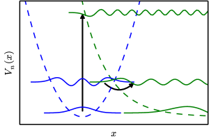
Figure 1: The model system potential energy surfaces (dashed lines) for diabatic states $\ket{n}=\ket{0}$ (blue) and $\ket{1}$ (green) with some representative vibronic states indicated by the real parts of their wave functions plotted with arbitrary amplitude at the corresponding energy. Two possible transitions from reactant to product states are indicated by black arrows, the curved one representing an energy-conserving transition, whereas the straight arrow represents a spurious transition. Note that as these transitions are not coupled with absorption or emission of radiation, only energy-conserving transitions contribute to the rate constant.

We note that this model is merely used to illustrate the problem of oscillatory correlation functions and the improvements made by the introduction of our modified flux-side correlation function formalism in the next section. An infinite-dimensional condensed-phase problem will also have a continuum of product states, Weiss (2008) and as already mentioned, it is simple to extend our analysis to include a nuclear-dependent coupling $\Delta(x)$. Our findings should therefore apply equally well to electron transfer in multidimensional complex systems.

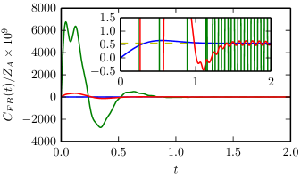
Figure 2: Three flux-side correlation functions for the model system: the symmetric version with $\beta^{\prime}=\tfrac{1}{2}\beta$ is shown in blue, the real part of the standard version with $\beta^{\prime}=0$ in green, and the Kubo transform in red. All three converge on the golden-rule rate (yellow dashed) in the long time limit as can be seen in some of the cases in the magnified inset.

We display the time-dependence of various flux-side correlation functions computed for the model system in Fig. 2. In the numerical calculations, we took a discrete set of product states and employed a cut-off for the highest-energy state considered. The Hamiltonian in the resulting finite basis was diagonalized to give the eigenstates from which the correlation function is calculated. The product-state density and cut-off were then increased until convergence of the results was achieved.

It is seen in the case of the unbiased system that at short times, the standard correlation function is extremely oscillatory with a large amplitude and plateaus to the correct rate constant only after a very long transient time (not shown in the figure). The symmetric version, on the other hand, is quite smooth and tends much sooner to its long-time limit. The Kubo transformed correlation function, which is an average of such correlation functions as these, is dominated by its integrand in the limits $\beta^{\prime}\rightarrow 0$ and $\beta^{\prime}\rightarrow\beta$ and, although totally real, is also strongly oscillatory at short times. We will describe functions as oscillatory if they at any time considerably overshoot their long-time limit.

Any numerical sampling procedure attempting to compute the rate constant from the Kubo-transformed or standard correlation functions will have significant numerical convergence problems. It is unfortunately exactly this type of correlation function that one would like to compute with trajectory simulations including nonadiabatic RPMD. Richardson and Thoss (2013) Many previous approaches have concentrated on computing the smoother symmetric correlation function, whether based on trajectories employing mapping variables, Wang et al. (1999) real-time path integrals Topaler and Makri (1996) or MCTDH. Wang, Skinner, and Thoss (2006) We note, however, that for lower temperatures or strongly biased systems, even the symmetric correlation function can become oscillatory and could cause problems for these methods as well. The onset of this regime is observed in the biased systems considered in LABEL:Wang2006flux and the real-time path-integral calculations of LABEL:Menzeleev2011ET and is discussed in LABEL:Huo2013PLDM.

What is needed is a new correlation function formalism from which the rate constant can rigorously be extracted from its long-time limit but which is not oscillatory at short times. We address this in the next section.

IV Non-oscillatory correlation functions

The causes of the oscillations in the flux-side correlation function are transitions between low-energy reactant states and high-energy product states which have a significant overlap in nuclear-configuration space. Of course, these spurious transitions have different phases and cancel out in the long-time limit leaving only energy-conserving transitions occurring between degenerate states, hence the appearance of the delta function in the golden-rule formula, Eq. (21). A schematic of transitions contributing to the short-time limit is given in Fig. 1. From the viewpoint of a trajectory-based method, the short-time limit would be dominated by trajectories hopping vertically from configurations deep in the reactant or product wells and not at the crossing of the potentials where one would expect reactive pathways to be located. It is well-known to be an ill-posed problem to cancel phases using numerical sampling methods, and thus the long-time limit would be very difficult to converge.

Rather than continuing to use the traditional flux-side formalism, we return to the general formula for the rate constant derived by linear response theory in Eq. (16) but retain the definitions of $A$ and $B$ from the previous section as projections onto the diabatic surfaces. We suggest the following modified nonequilibrium perturbation to avoid the oscillation problems at short times,

$$H_{1} =\iint\delta(H-E)\,B\,\delta(H-E^{\prime})\,\mathrm{e}^{-a^{2}(E-E^{\prime})^{2}}\mathrm{d}E\,\mathrm{d}E^{\prime}$$ (25a)

$$F_{a}\equiv\dot{H}_{1} =\iint\delta(H-E)\,F\,\delta(H-E^{\prime})\,\mathrm{e}^{-a^{2}(E-E^{\prime})^{2}}\mathrm{d}E\,\mathrm{d}E^{\prime},$$ (25b)

where the second line follows rigorously by virtue that $H$ commutes with the delta functions, and we have introduced a real-valued parameter $a$ with units of inverse energy. These expressions can be calculated exactly in the basis of eigenstates of $H$, which we call $\ket{i}$ with energy $E_{i}\equiv\braket{i}{H}{i}$, and obviously reduce to the traditional approach outlined in the previous section if $a=0$.

We will explain our reasons for choosing this particular form with an analysis of the behaviour of the modified correlation functions based on Eq. (25) in the strict golden-rule limit where a closed-form solution can be derived. Our findings should also give a good description of the behaviour in the weak-coupling regime.

It can easily be shown in the eigenstate basis that the important relation $\braket{H_{1}}=\braket{B}$ holds for any value of $a$. Therefore, in the slow reaction limit, neglecting $C_{H_{1}A}(t)$ as before, Craig, Thoss, and Wang (2007) we can compute the rate in terms of the modified flux-side or flux-flux correlation functions

$$k=Z_{A}^{-1}C_{F_{a}B}(t)=Z_{A}^{-1}\int_{0}^{t}C_{F_{a}F}(\tau)\,\mathrm{d}\tau.$$ (26)

This is analogous to the familiar flux correlation function formalism Miller, Schwartz, and Tromp (1983) and thanks to a derivation from the general rate expression Eq. (16), also rigorously gives the correct result for a slow reaction in the long-time limit for any value of $a$ and $\Delta$. In fact, it can be shown that the long-time limit of the rate formula Eq. (26) is unaffected by our introduction of the parameter $a$ by writing the modified flux-flux correlation function in the basis of eigenstates:

$$C^{\beta^{\prime}}_{F_{a}F}(t)=\sum_{ij}\mathrm{e}^{-\beta E_{j}+\beta^{\prime}\Delta E_{ij}}|\!\braket{i}{F}{j}\!|^{2}\,\mathrm{e}^{\mathrm{i}\Delta E_{ij}t/\hbar}\,\mathrm{e}^{-a^{2}\Delta E_{ij}^{2}},$$ (27)

where $\Delta E_{ij}=E_{j}-E_{i}$. Integration over time using the Fourier relation $\int_{-\infty}^{\infty}\mathrm{e}^{\mathrm{i}Et}\mathrm{d}t=2\pi\delta(E)$ shows that the long-time limits of $C^{\beta^{\prime}}_{F_{a}B}(t)$ and $C^{\beta^{\prime}}_{FB}(t)$ are rigorously equivalent. This therefore proves the equivalence of our modified flux correlation formalism and the traditional approach derived directly from scattering theory Miller, Schwartz, and Tromp (1983) without the need to use any of the assumptions inherent in linear response theory and nonequilibrium statistical mechanics.

We wish to analyse the effect that our modification has made to the correlation functions at short times, in particular in the weak-coupling limit. A simple expression for the modified flux operator, Eq. (25b), in terms of the reactant and product states can be derived only in the $\Delta\rightarrow 0$ limit, where the eigenstates of $H$ are only slightly perturbed from those of $H_{0}$, i.e. $\ket{i}\approx\ket{\mu_{i}}$ or $\ket{\nu_{i}}$ where $E_{i}\approx E_{\mu_{i}}$ or $E_{\nu_{i}}$. Any deviation from this approximation leads to higher orders of $\Delta$ and can thus be ignored in the golden-rule limit. This implies

$$\delta(H-E)\ket{\mu} =\sum_{i}\delta(H-E)\ket{i}\braket{i}{\mu}\approx\delta(E_{\mu}-E)\ket{\mu}$$ (28)

and its equivalent for product states, $\ket{\nu}$, such that

$$F_{a} \approx\frac{\mathrm{i}}{\hbar}\sum_{\mu\nu}\big{(}\ket{\mu}\Delta_{\mu\nu}\bra{\nu}-\ket{\nu}\Delta_{\nu\mu}\bra{\mu}\big{)}\,\mathrm{e}^{-a^{2}\Delta E_{\mu\nu}^{2}}.$$ (29)

It is noted that this approximation and hence the remainder of formulae in this section are only valid in the golden-rule limit and should not be used in general. The exact expression, Eq. (25b), is used in all the numerical calculations and the approximation only for the mathematical analysis.

It can now be more clearly seen why the particular form of $H_{1}$ introduced in Eq. (25) was chosen. The parameter $a>0$ can be chosen to ensure that only the reactant to product transitions which approximately conserve energy contribute to the modified flux operator. Note that in the $a\rightarrow\infty$ limit, the exponential becomes sharply peaked like a delta function such that only strictly energy-conserving transitions are allowed. It will become apparent that using this limit would have lead directly to the golden-rule rate as described in Sec. VI but that the parametrized version given here is more useful, because from it we can also derive a practical correlation function formalism for dynamical simulations.

We now analyse the correlation functions when using the modified flux. Describing the dynamics using first-order perturbation theory, or equivalently by retaining only terms of $O(\Delta^{2})$, which is exact in the golden-rule limit, we obtain

$$C^{\beta^{\prime}}_{F_{a}B}(t) =\frac{\mathrm{i}}{\hbar}\sum_{\mu\nu}\operatorname{Tr}\Big{[}\mathrm{e}^{-\beta^{\prime}H}\big{(}\ket{\mu}\Delta_{\mu\nu}\bra{\nu}-\ket{\nu}\Delta_{\nu\mu}\bra{\mu}\big{)}$$

$$\quad\times\mathrm{e}^{-(\beta-\beta^{\prime})H}\,\mathrm{e}^{\mathrm{i}Ht/\hbar}\ket{\nu}\!\bra{\nu}\mathrm{e}^{-\mathrm{i}Ht/\hbar}\Big{]}\mathrm{e}^{-a^{2}\Delta E_{\mu\nu}^{2}}$$ (30)

$$=\frac{1}{\hbar^{2}}\sum_{\mu\nu}\mathrm{e}^{-\beta E_{\mu}}|\Delta_{\mu\nu}|^{2}\int_{0}^{t}\mathrm{d}\tau\,\mathrm{e}^{-a^{2}\Delta E_{\mu\nu}^{2}}$$

$$\quad\Big{[}\mathrm{e}^{-(\beta-\beta^{\prime})\Delta E_{\mu\nu}}\mathrm{e}^{\mathrm{i}\Delta E_{\mu\nu}\tau/\hbar}+\mathrm{e}^{-\beta^{\prime}\Delta E_{\mu\nu}}\mathrm{e}^{-\mathrm{i}\Delta E_{\mu\nu}\tau/\hbar}\Big{]}.$$ (31)

The modified Kubo-transform is defined from this using Eq. (15).

We then assume that the product energy levels are continuous and that both the density of states and $\Delta_{\mu\nu}^{2}$ are slowly varying with $E_{\nu}$ for all transitions allowed from $\ket{\mu}$. Note that, as for the standard derivation of the golden-rule rate, by taking the long-time limit, in which the time-integral tends to a sharp peak about $\Delta E_{\mu\nu}=0$, this assumption can always be made true. In our case, this approximation is exact (in the golden-rule limit) not only for $t\rightarrow\infty$ but also at all times in the $a\rightarrow\infty$ limit when the integrand is localized about $\Delta E_{\mu\nu}=0$ by the Gaussian term. We therefore write

$$C^{\beta^{\prime}}_{F_{a}B}(t) \approx\frac{1}{\hbar^{2}}\sum_{\mu}\mathrm{e}^{-\beta E_{\mu}}|\Delta_{\mu\bar{\nu}}|^{2}\iint_{0}^{t}\mathrm{d}\tau\,\mathrm{d}\Delta E_{\mu\nu}\,\mathrm{e}^{-a^{2}\Delta E_{\mu\nu}^{2}}$$

$$\quad\Big{[}\mathrm{e}^{-(\beta-\beta^{\prime})\Delta E_{\mu\nu}}\mathrm{e}^{\mathrm{i}\Delta E_{\mu\nu}\tau/\hbar}+\mathrm{e}^{-\beta^{\prime}\Delta E_{\mu\nu}}\mathrm{e}^{-\mathrm{i}\Delta E_{\mu\nu}\tau/\hbar}\Big{]}$$ (32)

$$=\frac{1}{\hbar^{2}}\sum_{\mu}\mathrm{e}^{-\beta E_{\mu}}|\Delta_{\mu\bar{\nu}}|^{2}\frac{\sqrt{\pi}}{a}\int_{0}^{t}\mathrm{d}\tau$$

$$\quad\Big{[}\mathrm{e}^{-(\tau+\mathrm{i}\hbar(\beta-\beta^{\prime}))^{2}/4\hbar^{2}a^{2}}+\mathrm{e}^{-(\tau-\mathrm{i}\hbar\beta^{\prime})^{2}/4\hbar^{2}a^{2}}\Big{]}.$$ (33)

By evaluating the time integrals over the two half-Gaussians to give $\sqrt{\pi}\hbar a$, we recover the golden-rule rate Eq. (21) for any value of $a$. This is of course unsurprising as we have derived the result directly from linear response theory and taken only approximations valid in the $\Delta\rightarrow 0$ limit.

This analysis does not however apply at short times with small values of $a$. In this regime, the approximation that $|\Delta_{\mu\nu}|^{2}$ and the density of states are slowly varying does not in general hold and thus for example the symmetric function in Fig. 2 is rather tame contrary to what would be suggested by Eq. (33). However, as was shown numerically, the Kubo transform with $a=0$ is nonetheless oscillatory at short times, as are the symmetric functions in strongly-biased systems. Huo, Miller III, and Coker (2013) A better indicator of the short-time behaviour is provided by the gradient at $t=0$, equal to $C_{F_{a}F}(0)$, which is discussed in Secs. V and VI.1. From this it is seen that the initial gradient of the flux-side function will decrease as $a$ increases, which ensures that, for large enough $a$, the function does not overshoot its long-time limit at short times.

It is the presence of imaginary parts in the two exponential terms in Eq. (33) which leads to the oscillatory behaviour at long times observed in Fig. 2. We note that choosing $\beta^{\prime}=0$ or $\beta$ will make only one of the two terms non-oscillatory, and that the symmetrized version, $\beta^{\prime}=\tfrac{1}{2}\beta$, should give the least problematic form. The oscillations occur on a time scale of $O(\hbar a^{2}/\beta)$ with a Gaussian decay on a time scale of $O(\hbar a)$. The only universal method for damping these oscillations is to select a large value of $a$ on at least the same order of magnitude as $\beta$ such that the oscillation period is slower than the decay. In the limit $a\gg\beta$,

$$C_{F_{a}B}(t) =\frac{1}{\hbar^{2}}\sum_{\mu}\mathrm{e}^{-\beta E_{\mu}}|\Delta_{\mu\bar{\nu}}|^{2}\frac{\sqrt{\pi}}{a}2\int_{0}^{t}\mathrm{e}^{-\tau^{2}/4\hbar^{2}a^{2}}\mathrm{d}\tau$$ (34)

$$=\frac{2\pi}{\hbar}\sum_{\mu}\mathrm{e}^{-\beta E_{\mu}}|\Delta_{\mu\bar{\nu}}|^{2}\operatorname{Erf}(t/2\hbar a).$$ (35)

The error function, $\operatorname{Erf}(z)$, tends to 1 in the $z\rightarrow\infty$ limit and, as expected, recovers the golden-rule rate. As this result does not depend on the value of $\beta^{\prime}$, we have dropped the superscript from the correlation function.

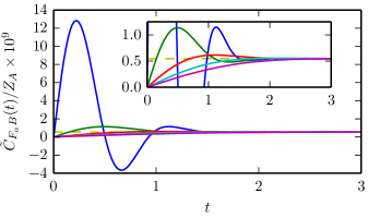
Figure 3: The Kubo-transformed modified flux-side correlation function for various values of $a$: blue $a=0.2$, green $a=0.4$, red $a=0.6$, cyan $a=0.8$, magenta $a=1$. All five converge to the golden-rule rate (yellow dashed) in the long time limit as can be seen in the magnified inset. Note that the $a=0$ version, shown in Fig. 2, is way off this scale.

Of course, this means that for very large $a$, it will be necessary to propagate to longer times to reach the plateau. Therefore for each problem, we should choose the minimum value of $a$ which defines a non-oscillatory function in order to achieve the best efficiency. We explore the effects of varying this parameter numerically in Fig. 3. It is seen that the Kubo correlation function, which had large oscillations for $a=0$ has been smoothed out using the parameter $a>0$, where it tends to the shape of an error function.

In the biased case, even the symmetric correlation function becomes oscillatory as shown in Fig. 4. We note that varying the value of $\beta^{\prime}$ only makes the problem worse, but that increasing $a$ removes the oscillations completely.

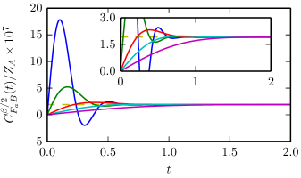
Figure 4: The symmetric correlation functions ($\beta^{\prime}=\tfrac{1}{2}\beta$) for a biased system with $\beta=1$, $\alpha=0.5$, $\epsilon=10$ for various values of $a$: blue $a=0$, green $a=0.1$, red $a=0.2$, cyan $a=0.3$, magenta $a=0.5$. All five converge to the golden-rule rate (yellow dashed) in the long time limit as can be seen in the magnified inset.

This completes our definition and study of the non-oscillatory flux-side correlation function formalism. In summary, due to the rigorous derivation from linear response theory, our modifications have not changed the long-time limit of the correlation functions from which the rate constant is defined, regardless of the strength of the electronic coupling parameter $\Delta$. However, the particular form of nonequilibrium perturbation used, Eq. (25), has removed the oscillatory problem in the weak-coupling limit. In the adiabatic, strong-coupling limit, the most efficient way to compute the rate is of course with none of these functions but with a position-dependent dividing surface. A complete nonadiabatic rate theory should be able to make use of both of these limits.

Note that we have not simply computed the oscillatory integral using a stationary-phase approximation but instead derived a non-oscillatory version which gives the exact rate. This is not only a more accurate approach but also leads to useful new developments. The non-oscillatory correlation function formalism is expected to be of great use in the development of new approximate dynamical methods. Immediate advances include an improved initial distribution for nonadiabatic classical trajectory simulations and a new formulation of the exact golden-rule rate in terms of the quantum trace. We deal with the former in the next section and the latter in Sec. VI.

V Modified initial distributions

As we have already discussed, a trajectory simulation of the traditional Kubo-transformed flux-side correlation function in the nonadiabatic, weak-coupling limit will be dominated by transitions occurring in the reactant or product wells leading to strong oscillations at short times. We know from the laws of energy conservation, that successful transitions should only occur in the region of the crossing point. However, neither the flux, $F$, nor a Kubo-transformed thermal flux operator localizes the initial distribution here. As we shall show, the modified flux, $F_{a}$, offers the possibility to alleviate this problem via the strength of the parameter $a$.

We shall consider here the classical limit of trajectory-based nonadiabatic dynamics simulations of one-dimensional systems, as this provides one of the simplest problems that poses a significant challenge to current methods. Landry and Subotnik (2012); Menzeleev, Bell, and Miller III (2014) By this limit, as discussed in LABEL:Tully1990hopping, we imply that the system is formed of heavy nuclei moving with small velocities but which are still allowed to hop between diabatic surfaces—an inherently quantum effect. We do not specify any particular form of trajectory method, or even if it gives exact or approximate dynamics. The extension to treat multidimensional systems with position-dependent electronic coupling is trivial and we leave the generalization for the treatment of quantum nuclei by path-integral methods to future work.

Let us assume that we wish to compute the Kubo-transformed modified flux-flux correlation function, $\tilde{C}_{F_{a}F}(t)$. The distribution of the initial nuclear coordinate contributing to the short-time limit is given by

$$\tilde{P}_{a}(x) =\frac{1}{\beta}\int_{0}^{\beta}\operatorname{Tr}\left[\mathrm{e}^{-\beta^{\prime}H}F_{a}\,\mathrm{e}^{-(\beta-\beta^{\prime})H}F\,\delta(\hat{x}-x)\right]\mathrm{d}\beta^{\prime},$$ (36)

such that $\tilde{C}_{F_{a}F}(0)=\int_{-\infty}^{\infty}\tilde{P}_{a}(x)\,\mathrm{d}x$.

In order to put this into closed form, where we can more easily study the properties of the distribution, we substitute quantum operators for localized classical variables to give an approximation to the modified flux

$$F_{a} \approx\frac{\mathrm{i}\Delta}{\hbar}\iint\delta(p^{2}/2m+V(x)-E)\,\big{(}\ket{0}\!\bra{1}-\ket{1}\!\bra{0}\big{)}$$

$$\quad\times\delta(p^{2}/2m+V(x)-E^{\prime})\,\mathrm{e}^{-a^{2}(E-E^{\prime})^{2}}\mathrm{d}E\,\mathrm{d}E^{\prime}.$$ (37)

The integrals can be performed at each value of $x$ in the basis of adiabatic electronic states $\ket{\chi_{\pm}(x)}$, which diagonalize the diabatic potential matrix $V(x)$. The corresponding eigenvalues are $W_{\pm}(x)\equiv\braket{\chi_{\pm}(x)}{V(x)}{\chi_{\pm}(x)}$. Using the relations given in Appendix C along with standard trigonometric identities, we can show that it simplifies to give

$$F_{a}\approx\frac{\mathrm{i}\Delta}{\hbar}\big{(}\ket{0}\!\bra{1}-\ket{1}\!\bra{0}\big{)}\,\mathrm{e}^{-a^{2}[W_{+}(x)-W_{-}(x)]^{2}}.$$ (38)

It is seen that the modified flux, within the classical approximation, is simply the standard flux operator weighted by a Gaussian which localizes it about the avoided crossing.

The classical distribution contributing to $\tilde{C}_{F_{a}F}(0)$ is obtained in the same way to give

$$\tilde{P}_{a}(x)\approx\sqrt{\frac{m}{2\pi\beta\hbar^{2}}}\frac{2\Delta^{2}}{\beta\hbar^{2}}\frac{\mathrm{e}^{-\beta W_{-}(x)}-\mathrm{e}^{-\beta W_{+}(x)}}{W_{+}(x)-W_{-}(x)}\\ \times\mathrm{e}^{-a^{2}[W_{+}(x)-W_{-}(x)]^{2}}.$$ (39)

In the golden-rule limit, i.e. retaining only terms of order $\Delta^{2}$, this becomes

$$\tilde{P}_{a}(x)\approx\sqrt{\frac{m}{2\pi\beta\hbar^{2}}}\frac{2\Delta^{2}}{\beta\hbar^{2}}\frac{\mathrm{e}^{-\beta V_{1}(x)}-\mathrm{e}^{-\beta V_{0}(x)}}{V_{0}(x)-V_{1}(x)}\\ \times\mathrm{e}^{-a^{2}[V_{0}(x)-V_{1}(x)]^{2}}.$$ (40)

It is from distribution functions such as these that initial points are selected for trajectory simulations. *[Thesamplingofacorrelationfunctionusingadistributionbasedonitszero-timelimitisdiscussedin][]Zimmermann2013sampling Note that in order to sample these functions, it would not be necessary to know the exact location of the crossing of the potentials which for a complex multidimensional system would be a high-dimensional hypersurface and is generally difficult to calculate. Instead, a Monte Carlo evaluation would automatically select samples from the correct region of configuration space. The distribution at the same level of approximation corresponding to the original unmodified Kubo-transformed flux-flux correlation function, $\tilde{P}_{0}(x)$, is found by setting $a=0$. A range of approximate modified distributions with $a\geq 0$ are presented in Fig. 5 for a biased and an unbiased system.

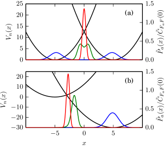
Figure 5: Normalized classical nuclear distributions, $\tilde{P}_{a}(x)$, in the golden-rule limit, Eq. (40), for initializing a Kubo-transformed modified flux-flux correlation function calculation; $a$ is equal to 0 (blue), 0.15 (green) or 0.3 (red). The system is a typical two-state curve-crossing problem, Eq. (59), with diabatic surfaces shown in black, $\beta=1$ no bias in the top panel and $\epsilon=30$ in the lower.

It is seen that large values of $a$ localize the nuclear distribution about the crossing point with an effective localization given by

$$\frac{\tilde{P}_{a}(x)}{\tilde{P}_{0}(x)}\approx\mathrm{e}^{-a^{2}[W_{+}(x)-W_{-}(x)]^{2}}.$$ (41)

This effect applies equally to symmetric as to biased systems even deep into the inverted regime. This is exactly the effect that we wished to apply to the system based on an intuition that trajectories should hop between diabatic surfaces only in this region. Estimates for good values of $a$ can be obtained from an analysis of the golden-rule limit of the approximate distribution function, given by Eq. (40). We here assume that the system has strong vibronic coupling such that $\beta V_{n}^{\prime}(x^{\ddagger})^{2}\gg V_{n}^{\prime\prime}(x^{\ddagger})$, where $x^{\ddagger}$ is the crossing point such that $V_{0}(x^{\ddagger})=V_{1}(x^{\ddagger})$. The distribution in a symmetric system has a maximum at $x=0$ for $a\geq\beta/\sqrt{24}$. For an asymmetric system, the distribution at $x^{\ddagger}$ is not necessarily a stationary point but has a negative curvature, and is therefore well within the envelope, for $a\geq\beta\sqrt{1/6+V_{0}^{\prime}(x^{\ddagger})V_{1}^{\prime}(x^{\ddagger})/2\mathcal{F}^{2}}$, where $\mathcal{F}=|V_{0}^{\prime}(x^{\ddagger})-V_{1}^{\prime}(x^{\ddagger})|$. We note that the value of $a$ used in simulations can be chosen to minimize oscillations and optimize the efficiency of the calculation and that these estimates may be used for a good first guess and do not need to be accurately calculated. In principle, the rate constant found by an accurate simulation will not depend on the value chosen.

With an exact dynamical method, one could therefore compute the modified flux-flux correlation function, and hence the rate constant, starting from a localized region of configuration space. Note that the localization has appeared naturally from our derivation from linear response theory. We could not have simply performed Monte Carlo importance sampling of $\tilde{P}_{0}(x)$ with an umbrella function centred about the crossing point because this would still be a simulation of the original correlation function, and in fact the effects of outlying trajectories which do start in the wells would be magnified by the umbrella and worsen the statistics even more. Although a nuclear-configurational dividing surface could also be used to localize the nuclei at the crossing point, as discussed above, such dividing-surface approaches lead to inefficient calculations due to its time derivative, the flux, which depends on the nuclear momenta rather than diabatic hops.

It was possible for previous studies Topaler and Makri (1996); Wang et al. (1999); Wang, Skinner, and Thoss (2006) to perform efficient simulations of symmetric correlation functions without the present modifications. This is because the symmetrized thermal flux $\mathrm{e}^{-\beta H/2}F\mathrm{e}^{-\beta H/2}$, unlike its Kubo-transformed version, is localized about $x=0$ for a spin-boson model. However, for strongly biased systems, Menzeleev, Ananth, and Miller (2011); Huo, Miller III, and Coker (2013) this does not coincide with the diabatic crossing point, $x^{\ddagger}$, and the current theory may be useful to avoid strongly oscillatory functions.

In conclusion, the proposed modified flux-side correlation functions $C_{F_{a}B}(t)$ can be used instead of the original flux-side versions $C_{FB}(t)$ as they all tend to the same long-time limit from which the rate constant is given exactly. Therefore, for an exact dynamical method based on flux correlation functions, and in particular the Kubo-transformed versions, the proposed modifications will improve the efficiency without affecting the result, regardless of the strength of electronic coupling. Approximate methods will also see a large efficiency gain and may even see an improvement in the accuracy of their results as phase cancellation is no longer necessary with this more intuitive localized initial distribution. Such applications will be explored in future work.

VI Golden-rule transition-state theory

VI.1 Quantum formulation

The modified nonequilibrium perturbation, Eq. (25), was introduced in order to damp the oscillations of the flux correlation functions, but we shall show that it can also be used to derive a new formulation of a nonadiabatic quantum transition-state theory, which is exact in the golden-rule limit.

There are many different theories in the literature bearing the TST label, often with quite different meanings. We use the definition that TST is a dynamics-free approach based on the statistical mechanics of a low-probability region of phase space associated with transitions—in this case, near the crossing point where the diabatic potentials are equal. There must also exist a related correlation function from which the exact rate can be computed and which is equivalent to the TST rate if there is no recrossing in the dynamics.

The definition of recrossing in the correlation function varies depending on the system studied. For example, for adiabatic dynamics, a dividing surface in nuclear-configuration space is usually defined and the TST assumption is that trajectories will never cross this dividing surface more than once. For the classical Born-Oppenheimer flux-side correlation function Chandler (1978, 1987) and a particular generalization of its quantum equivalent, Hele and Althorpe (2013a); *Althorpe2013QTST it can be shown that the non-recrossing assumption leads to a step-like shape and therefore that the TST rate is proportional to its $t\rightarrow 0_{+}$ limit.

In our case, where there is no dividing surface, a recrossing path will be defined as one which hops between the diabatic states more than once within either the forward or backward propagators $\mathrm{e}^{\mp\mathrm{i}Ht/\hbar}$. Because each hop introduces a factor of $\Delta$, this non-recrossing assumption is exact in the golden-rule limit. For a system with a continuum of product states in the $\Delta\rightarrow 0$ limit, it was seen in Eq. (35) that the correlation function $C_{F_{a}B}(t)$ with $a\rightarrow\infty$ goes like the error function and that therefore its time-derivative, the modified flux-flux correlation function, $C_{F_{a}F}(t)$ is Gaussian with known width. We can therefore use this as our correlation function from which the exact rate can be computed whether the non-recrossing assumption is valid or not, but which, in the golden-rule limit, has a simple form from which we can compute the TST rate solely from its value at $t=0$. As was shown in the previous section, the corresponding distribution will be localized about the crossing region. Like other quantum TSTs,Hele and Althorpe (2013a) our formulation will not necessarily be variational, i.e. the exact rate may be smaller or larger than the TST rate.

According to our definition, the approach of Wolynes Wolynes (1987) is not a TST but instead a quantum instanton approximation as it is based on a steepest-descent integration along time. Vaníček et al. (2005) It is therefore not necessarily exact for a system with no recrossing, that is in the golden-rule $\Delta\rightarrow 0$ limit, and is not directly related to a dynamical method.

In order to formulate a quantum expression for the golden-rule TST rate, we utilize the fact that we know the shape of the modified flux-flux correlation function in the limit $a\rightarrow\infty$ within the non-recrossing assumption. That is

$$\lim_{a\rightarrow\infty}C_{F_{a}F}(t) \approx\lim_{a\rightarrow\infty}C_{F_{a}F}(0)\,\mathrm{e}^{-t^{2}/4\hbar^{2}a^{2}},$$ (42)

where the approximation becomes exact in the $\Delta\rightarrow 0$ limit. The value at zero time for any value of $\beta^{\prime}$ is given by

$$C_{F_{a}F}(0) =\operatorname{Tr}\left[\mathrm{e}^{-\beta^{\prime}H}F_{a}\,\mathrm{e}^{-(\beta-\beta^{\prime})H}F\right]$$ (43)

$$\equiv\frac{2\sqrt{\pi}\Delta^{2}}{\hbar^{2}a}\mathcal{Z}^{\ddagger}(a)$$ (44)

where $\mathcal{Z}^{\ddagger}(a)$ is defined by this equivalence. We introduce the transition-state partition function

$$Z^{\ddagger} =\lim_{a\rightarrow\infty}\mathcal{Z}^{\ddagger}(a)$$ (45)

$$=\lim_{a\rightarrow\infty}\frac{a}{2\sqrt{\pi}}\iint\mathrm{d}E\,\mathrm{d}E^{\prime}\,\mathrm{e}^{-a^{2}(E-E^{\prime})^{2}}\lim_{\Delta\rightarrow 0}$$

$$\quad\operatorname{Tr}\Big{[}\mathrm{e}^{-\beta^{\prime}H}\delta(H-E)\ket{0}\!\bra{1}\delta(H-E^{\prime})\,\mathrm{e}^{-(\beta-\beta^{\prime})H}\ket{1}\!\bra{0}$$

$$\quad+\mathrm{e}^{-\beta^{\prime}H}\delta(H-E)\ket{1}\!\bra{0}\delta(H-E^{\prime})\,\mathrm{e}^{-(\beta-\beta^{\prime})H}\ket{0}\!\bra{1}\Big{]}$$ (46)

$$=\int\mathrm{e}^{-\beta E}\lim_{\Delta\rightarrow 0}\operatorname{Tr}\big{[}\delta(H-E)\ket{0}\!\bra{1}\delta(H-E)\ket{1}\!\bra{0}\big{]}\mathrm{d}E$$ (47)

$$=\int\mathrm{e}^{-\beta E}\operatorname{tr}\big{[}\delta\big{(}\!\braket{0}{H}{0}-E\big{)}\,\delta\big{(}\!\braket{1}{H}{1}-E\big{)}\big{]}\mathrm{d}E,$$ (48)

in which we have used a relation for the Dirac delta function $\delta(z)=\lim_{a\rightarrow\infty}\frac{a}{\sqrt{\pi}}\mathrm{e}^{-a^{2}z^{2}}$ and performed the integration over $E^{\prime}$. In the last line, the quantum trace is taken only over nuclear degrees of freedom.

The golden-rule TST rate is therefore

$$k_{\mathrm{TST}} =Z_{A}^{-1}\lim_{a\rightarrow\infty}\int_{0}^{\infty}C_{F_{a}F}(0)\,\mathrm{e}^{-\tau^{2}/4\hbar^{2}a^{2}}\mathrm{d}\tau$$ (49)

$$=\frac{2\pi\Delta^{2}}{\hbar}\frac{Z^{\ddagger}}{Z_{A}}.$$ (50)

This expression is only valid in the $\Delta\rightarrow 0$ limit where it gives the quantum golden-rule result exactly but without explicitly using the states of the system. This is most easily seen by evaluating the trace in the basis of the vibronic states before integrating over energy from which Eq. (21) is recovered. It is however a more general result which also applies to complex systems after a trivial extension to multidimensional nuclear configurations and non-constant electronic coupling $\Delta(\hat{x})$, which would then be included inside the trace of Eq. (48).

We could have derived this result from an alternative formulation of the rate constant in terms of the microcanonical cumulative reaction probability, equivalent to that of LABEL:Miller1983rate with a substitution for the electronic flux, Eq. (20a):

$$k=\frac{\pi\hbar}{Z_{A}}\int\mathrm{e}^{-\beta E}\operatorname{Tr}\big{[}F\delta(E-H)F\delta(E-H)\big{]}\mathrm{d}E.$$ (51)

This general formulation gives the exact rate constant regardless of the coupling strength, $\Delta$, and reduces to our TST result, Eq. (50), in the $\Delta\rightarrow 0$ limit. However, the new derivation presented in this work has shown that the golden-rule result can be considered a transition-state theory in the sense that it can be linked to the short-time limit of the modified flux-flux correlation function in the $a\rightarrow\infty$ limit. Such links with transition-state theories can be invaluable when developing new trajectory-based methods for rate calculations.

The new formulation, Eq. (50), can be compared to the imaginary-time path-integral methods for computing the golden-rule rate of Refs. Wolynes, 1987; Cao and Voth, 1997. They also depend on a transition-state partition function where two diabatic hops are enforced but without explicitly imposing energy conservation. These methods were derived from a steepest-descent approximation to the analytically-continued flux-flux correlation function formalism and are not exact, even in the golden-rule limit. Our new formulation does not take these approximations and also avoids the unsavoury analytic continuation.

We note that unlike the former approaches, for which results are efficiently computed using path-integral Monte Carlo, at first glance, a numerical evaluation of Eq. (48) using path integrals Chandler and Wolynes (1981); Wolynes (1987); Alexander (2001) or semiclassical instanton methods Miller (1975a); Cao and Voth (1997) looks extremely complicated due to presence of the microcanonical density operators. Miller (1975b); Lawson (2000) However, it is simplified somewhat by the integral over energy. Further work will assess whether a practical formulation can be found applicable to complex systems. We can however analyse quite easily the classical limit which is outlined in the next section.

VI.2 Classical golden-rule rate

In the limiting case that the one-dimensional nuclear motion can be considered classically, we can show that the TST formulation derived above gives the same rate constant as Landau-Zener theory or, in the special case of a spin-boson system, Marcus theory.

We take the classical limit of Eq. (48) as in Sec. V to give

$$Z^{\ddagger} =\frac{1}{2\pi\hbar}\int\mathrm{d}E\,\mathrm{e}^{-\beta E}\iint_{-\infty}^{\infty}\mathrm{d}x\,\mathrm{d}p$$

$$\quad\times\delta\big{(}p^{2}/2m+V_{0}(x)-E\big{)}\,\delta\big{(}p^{2}/2m+V_{1}(x)-E\big{)}$$ (52)

$$=\frac{1}{2\pi\hbar}\iint_{-\infty}^{\infty}\mathrm{e}^{-\beta p^{2}/2m}\,\mathrm{e}^{-\beta V_{0}(x)}\,\delta\big{[}V_{0}(x)-V_{1}(x)\big{]}\,\mathrm{d}x\,\mathrm{d}p,$$ (53)

where here $x$ and $p$ are considered as classical variables. This same result could also be derived from the classical limit Lawson (2000) of the elements of the quantum microcanonical density matrix. Miller (1975b) Note that the two kinetic energy terms are equal in Eq. (VI.2), and have therefore cancelled out in the delta function in Eq. (53). This is because the flux operator does not affect position or momentum, only electronic states.

We proceed using

$$\delta\big{[}V_{0}(x)-V_{1}(x)\big{]}=\frac{\delta(x-x^{\ddagger})}{|V_{0}^{\prime}(x^{\ddagger})-V_{1}^{\prime}(x^{\ddagger})|}$$ (54)

and by defining the activation energy as $V^{\ddagger}\equiv V_{0}(x^{\ddagger})=V_{1}(x^{\ddagger})$ to give, from Eq. (50), a general formula for the classical TST rate,

$$k_{\mathrm{cl,TST}} =\sqrt{\frac{2\pi m}{\beta\hbar^{2}}}\frac{\Delta^{2}}{\hbar|V_{0}^{\prime}(x^{\ddagger})-V_{1}^{\prime}(x^{\ddagger})|}\frac{\mathrm{e}^{-\beta V^{\ddagger}}}{Z_{A}},$$ (55)

which is the same result as found by the Landau-Zener approach in the golden-rule limit for a one-dimensional system Nitzan (2006)

$$k_{\mathrm{LZ}} =\int_{-\infty}^{\infty}|\dot{x}|P(x^{\ddagger},\dot{x})P_{0\rightarrow 1}^{\ddagger}(\dot{x})\,\mathrm{d}\dot{x},$$ (56)

with Zener (1932)

$$P(x^{\ddagger},\dot{x}) =\frac{m}{2\pi\hbar Z_{A}}\,\mathrm{e}^{-\frac{1}{2}\beta m\dot{x}^{2}}\mathrm{e}^{-\beta V^{\ddagger}}$$ (57)

$$P^{\ddagger}_{0\rightarrow 1}(\dot{x}) =\frac{2\pi\Delta^{2}}{\hbar|\dot{x}||V^{\prime}_{0}(x^{\ddagger})-V_{1}^{\prime}(x^{\ddagger})|}.$$ (58)

Note that we have assumed that reactive trajectories can occur with positive or negative velocity, $\dot{x}$, as is appropriate for bound reactant states.

As a specific example, we consider a model system typically used in Marcus’ theory of electron-transfer reactions, defined as in Eq. (22) but with two harmonic potential energy surfaces Weiss (2008)

$$V_{0}(x) =\tfrac{1}{2}m\omega^{2}(x+x_{0})^{2},$$ (59a)

$$V_{1}(x) =\tfrac{1}{2}m\omega^{2}(x-x_{0})^{2}-\epsilon.$$ (59b)

The reorganization energy is $\Lambda=2m\omega^{2}x_{0}^{2}$ and the crossing point is $x^{\ddagger}=-x_{0}\epsilon/\Lambda$ with $V^{\ddagger}=(\Lambda-\epsilon)^{2}/4\Lambda$ and $V_{0}^{\prime}(x^{\ddagger})-V_{1}^{\prime}(x^{\ddagger})=\Lambda/x_{0}$. The reactant partition function is $Z_{A}=(\beta\hbar\omega)^{-1}$ and the rate constant predicted by Eq. (53) is

$$k_{\mathrm{cl,TST}} =\frac{\Delta^{2}}{\hbar}\sqrt{\frac{\pi\beta}{\Lambda}}\,\mathrm{e}^{-\beta(\Lambda-\epsilon)^{2}/4\Lambda}.$$ (60)

This is equal to the familiar classical Marcus rate, Marcus (1956) which is the result for a spin-boson system in the golden-rule limit with classical nuclei.

This link to Marcus theory is perhaps more exciting than it at first seems because, as already discussed, the path-integral golden-rule rate formula proposed by Wolynes, Wolynes (1987) Cao and Voth Cao and Voth (1997) cannot describe the correct behaviour in the inverted regime $\epsilon>\Lambda$. This shows that the current formulation, Eq. (50), is a more powerful starting point for the derivation of nonadiabatic golden-rule TST than the analytic-continuation or $\operatorname{Im}F$ methods.

Although the classical formula has reduced to well-known results, its formulation offers something new, which is a direct link between the non-dynamical Marcus theory and an exact correlation function formalism, showing that Marcus theory itself, and its anharmonic generalization Eq. (55), can be thought of as classical nonadiabatic transition-state theories. This implies that if a classical trajectory-based dynamical method, which may be efficiently initialized near the crossing-point, gives the correct Gaussian decay of the modified flux-flux correlation function in the large $a$ limit, it will necessarily reproduce rates of Marcus theory when in the golden-rule limit. This sets a very clear goal for the development of new nonadiabatic dynamical theories.

We note also that a multidimensional extension to Eq. (53) is found trivially by following the same procedure, which when combined with the usual efficient approaches for the calculation of free energies, gives perhaps one of the simplest methods for computing classical golden-rule rates without making the harmonic approximation.

VII Conclusions

We have analysed the use of the Kubo-transformed flux-side correlation function, with reactants and products defined as usual by projections onto electronic states, Topaler and Makri (1996) to compute the nonadiabatic rate constant for systems with weak electronic coupling. It was shown to be very inefficient due to strong oscillatory behaviour stemming from spurious diabatic transitions occurring between low- and high-energy states, which due to phase cancellation at long times do not contribute to the rate constant. Using a formalism based on linear response theory, we have proposed a modified flux-side correlation function which rigorously gives the same exact rate in the long-time limit, regardless of the electronic coupling strength, but which includes a parameter $a$ which can be chosen to remove the oscillations at short times. An alternative derivation equates the formalism directly with quantum scattering theory via the traditional flux correlation functions. Miller, Schwartz, and Tromp (1983)

Non-zero values of the parameter change the nuclear distribution function used to initialize typical trajectory simulations such that the distribution is localized about the crossing of the potential energy surfaces. Very large values of $a$ may need a longer propagation time to reach a plateau so we recommend a medium value of $a\sim\beta$ which would give an initial distribution of nuclear configurations distributed close to the crossing where the electronic states have similar energies. For complex systems, it will not of course be possible to compute the modified flux correlation functions exactly, any more than it is for the original form. However, the new formalism provides a rigorous base on which to build approximate dynamical methods, which share the benefits of being non-oscillatory and of starting from a distribution localized about the crossing point. Such methods will be more efficient and perhaps even more accurate due to the proposed modifications.

The new formalism is of particular importance for the use of nonadiabatic RPMD Richardson and Thoss (2013) in the weak-coupling regime, which like all ring-polymer approaches, Craig and Manolopoulos (2004) approximately computes Kubo-transformed correlation functions. The Kubo transform is also the most appropriate form for other classical-trajectory approaches as it shares many symmetry properties with classical correlation functions. Craig and Manolopoulos (2004) Further work will attempt to compute the non-oscillatory flux-side correlation functions using such approaches. However, it may also be possible to use the proposed function to improve the efficiency of a wide range of other nonadiabatic dynamical methods Wang, Skinner, and Thoss (2006); Topaler and Makri (1996); Wang et al. (1999) based on the symmetric correlation function at least when studying strongly biased systems. Menzeleev, Ananth, and Miller (2011); Huo, Miller III, and Coker (2013)

Our study of the initial distribution for trajectory simulations was based on a classical limit. Path-integral methods could be used for example to initialize nonadiabatic ring-polymer dynamics from Eq. (36) but further work is required before a practical path-integral sampling scheme can be implemented. We note, however, that even without this extension, there is still a large applicability for trajectory methods for the nonadiabatic dynamics of classical nuclei, using for example surface-hopping or classical mapping approaches. In fact, even the nonadiabatic RPMD method Richardson and Thoss (2013) with classical nuclei is worthy of study because the introduction of ring-polymer beads was seen not only to describe nuclear quantum effects but also to improve the electronic dynamics; i.e. it does not reduce to the classical $N=1$ mapping approach when the ring polymers collapse in nuclear-configuration space. There is therefore good reason to attempt to utilize such methods to compute the modified flux-side correlation functions proposed here.

We were also able to extract another useful development from the non-oscillatory correlation function formalism, which is the derivation of an expression for a nonadiabatic TST rate constant, exact in the golden-rule, $\Delta\rightarrow 0$, limit. This limit is often encountered in electron-transfer processes in the condensed phase, Chandler (1998) the simulation of which would provide many possible applications for the method. If the nuclei are considered to be classical and are treated in the harmonic approximation, the expression reduces to the Marcus theory rate even in the inverted regime. Further work is needed to find a practical expression for computer simulation which will allow the efficient computation of nonadiabatic rates in the golden-rule limit for complex systems including quantum-mechanical effects such as nuclear tunnelling in proton-coupled electron transfer. Hammes-Schiffer and Stuchebrukhov (2010)

VIII Acknowledgement

The authors would like to thank Stuart C. Althorpe for helpful comments on the manuscript. JOR gratefully acknowledges a Research Fellowship from the Alexander von Humboldt Foundation.

Appendix A Vibronic states

We define the one- or multidimensional nuclear configuration as $x$ and the positions of all electrons in the system as $\mathbf{r}$. As these variables cover all spatial degrees of freedom in a molecular system, we recognize the identity $\iint\ket{x,\mathbf{r}}\!\bra{x,\mathbf{r}}\mathrm{d}x\,\mathrm{d}\mathbf{r}=1$.

Writing the electronic (diabatic) wave functions as $\phi_{0}(\mathbf{r};x)$ and $\phi_{1}(\mathbf{r};x)$ and nuclear wave functions as $\psi_{\mu}(x)$ and $\psi_{\nu}(x)$, we can define the vibronic states using

$$\braket{x,\mathbf{r}}{\mu} =\psi_{\mu}(x)\phi_{0}(\mathbf{r};x), \braket{x,\mathbf{r}}{0} =\bra{x}\phi_{0}(\mathbf{r};x),$$

$$\braket{x,\mathbf{r}}{\nu} =\psi_{\nu}(x)\phi_{1}(\mathbf{r};x), \braket{x,\mathbf{r}}{1} =\bra{x}\phi_{1}(\mathbf{r};x).$$

Projections onto the electronic states give

$$\braket{0}{\mu} =\int\ket{x}\psi_{\mu}(x)\,\mathrm{d}x, \braket{1}{\nu} =\int\ket{x}\psi_{\nu}(x)\,\mathrm{d}x.$$

The coupling matrix element can therefore be defined as

$$\braket{\mu}{0}\braket{1}{\nu} =\iint\psi_{\mu}(x^{\prime})^{*}\braket{x^{\prime}}{x}\psi_{\nu}(x)\,\mathrm{d}x\,\mathrm{d}x^{\prime}$$ (61)

$$=\int\psi_{\mu}(x)^{*}\psi_{\nu}(x)\,\mathrm{d}x,$$ (62)

which is the Franck-Condon matrix element.

Appendix B Wave functions of the model system

The reactant well, Eq. (23), has the form of a harmonic oscillator with eigenstates

$$\psi_{\mu}(x)=\left(\frac{m\omega}{\pi\hbar}\right)^{\frac{1}{4}}\frac{1}{\sqrt{2^{\mu}\mu!}}\,\mathrm{e}^{-m\omega x^{2}/2\hbar}H_{\mu}\left(\sqrt{\frac{m\omega}{\hbar}}x\right),$$ (63)

where $\mu\in\{0,1,\dots\}$ and $H_{\mu}$ are the Hermite polynomials. The discrete energies are $E_{\mu}=(\mu+\tfrac{1}{2})\hbar\omega$.

The product wave functions are the continuum states of the repulsive Morse oscillator, Eq. (24), normalized in energy space, Mündel and Domcke (1984)

$$\psi_{\nu}(x)=\sqrt{\frac{m\hbar}{2\pi py}}(2b)^{-\zeta}\frac{\Gamma(\tfrac{1}{2}-\zeta)}{\Gamma(-2\zeta)}W_{0,\zeta}(y),$$ (64)

for $E_{\nu}>-\epsilon$, where $p=\sqrt{2m(E_{\nu}+\epsilon)}$, $b=\sqrt{2mD}/\hbar\alpha$, $\zeta=\mathrm{i}p/\hbar\alpha$ and $y=2b\exp[-\alpha(x-x_{0})]$. This particular Whittaker function is related [SeeEq.9.235.2from][]Gradshteyn to a modified Bessel function of purely imaginary order, $W_{0,\zeta}(y)=\sqrt{y/\pi}K_{\zeta}(y/2)$, which can be can be computed with the algorithm of LABEL:Gil2004iBessel.

Appendix C Adiabatic states

The adiabatic states $\ket{\chi_{\pm}(x)}$ are defined in the diabatic basis as the eigenvectors of the $2\times 2$ diabatic matrix $V(x)$, given by Eq. (22b). One can show Tannor (2007) that

$$\braket{0}{\chi_{+}(x)} =\cos\tfrac{\theta}{2} \braket{0}{\chi_{-}(x)} =-\sin\tfrac{\theta}{2}$$

$$\braket{1}{\chi_{+}(x)} =\sin\tfrac{\theta}{2} \braket{1}{\chi_{-}(x)} =\cos\tfrac{\theta}{2}$$

is the solution with

$$\tan\theta=\frac{2\Delta}{V_{0}(x)-V_{1}(x)}.$$ (65)

The corresponding eigenvalues are

$$W_{\pm}(x)=\frac{V_{0}(x)+V_{1}(x)}{2}\pm\tfrac{1}{2}\sqrt{[V_{0}(x)-V_{1}(x)]^{2}+4\Delta^{2}}.$$ (66)

References

- Tully (2012) J. C. Tully, J. Chem. Phys. 137, 22A301 (2012).
- Domcke, Yarkony, and Köppel (2004) W. Domcke, D. R. Yarkony, and H. Köppel, eds., Conical Intersections: Electronic Structure, Dynamics and Spectroscopy (World Scientific, Singapore, 2004).
- Levine and Martínez (2007) B. G. Levine and T. J. Martínez, Annu. Rev. Phys. Chem. 58, 613 (2007).
- Stock and Thoss (2005) G. Stock and M. Thoss, Adv. Chem. Phys. 131, 243 (2005).
- Garg, Onuchic, and Ambegaokar (1985) A. Garg, J. N. Onuchic, and V. Ambegaokar, J. Chem. Phys. 83, 4491 (1985).
- Leggett et al. (1987) A. J. Leggett, S. Chakravarty, A. T. Dorsey, M. P. A. Fisher, A. Garg, and W. Zwerger, Rev. Mod. Phys. 59, 1 (1987).
- Rips and Pollak (1995) I. Rips and E. Pollak, J. Chem. Phys. 103, 7912 (1995).
- Weiss (2008) U. Weiss, Quantum Dissipative Systems, 3rd ed. (World Scientific, Sinagpore, 2008).
- Wang, Thoss, and Miller (2001) H. Wang, M. Thoss, and W. H. Miller, J. Chem. Phys. 115, 2979 (2001).
- Thoss, Wang, and Miller (2001) M. Thoss, H. Wang, and W. H. Miller, J. Chem. Phys. 115, 2991 (2001).
- Wang and Thoss (2003) H. Wang and M. Thoss, J. Chem. Phys. 119, 1289 (2003).
- Thoss and Wang (2006) M. Thoss and H. Wang, Chem. Phys. 322, 210 (2006).
- Wang, Skinner, and Thoss (2006) H. Wang, D. E. Skinner, and M. Thoss, J. Chem. Phys. 125, 174502 (2006).
- Mak and Chandler (1991) C. H. Mak and D. Chandler, Phys. Rev. A 44, 2352 (1991).
- Topaler and Makri (1996) M. Topaler and N. Makri, J. Phys. Chem. 100, 4430 (1996).
- Mühlbacher and Egger (2003) L. Mühlbacher and R. Egger, J. Chem. Phys. 118, 179 (2003).
- Mühlbacher and Egger (2004) L. Mühlbacher and R. Egger, Chem. Phys. 296, 193 (2004).
- Zwanzig (2001) R. Zwanzig, Nonequilibrium Statistical Mechanics (Oxford University Press, 2001).
- Lee, Dunietz, and Geva (2013) M. H. Lee, B. D. Dunietz, and E. Geva, J. Phys. Chem. C 117, 23391 (2013).
- Bader, Kuharski, and Chandler (1990) J. S. Bader, R. A. Kuharski, and D. Chandler, J. Chem. Phys. 93, 230 (1990).
- Marcus (1956) R. A. Marcus, J. Chem. Phys. 24, 966 (1956).
- Chandler (1998) D. Chandler, in Classical and Quantum Dynamics in Condensed Phase Simulations, edited by B. J. Berne, G. Ciccotti, and D. F. Coker (World Scientific, Singapore, 1998) Chap. 2, pp. 25–49.
- Miller, Calcaterra, and Closs (1984) J. R. Miller, L. T. Calcaterra, and G. L. Closs, J. Am. Chem. Soc. 106, 3047 (1984).
- Egorov, Rabani, and Berne (1999) S. A. Egorov, E. Rabani, and B. Berne, J. Phys. Chem. B 103, 10978 (1999).
- Shi and Geva (2004) Q. Shi and E. Geva, J. Phys. Chem. A 108, 6109 (2004).
- Wolynes (1987) P. G. Wolynes, J. Chem. Phys. 87, 6559 (1987).
- Cao and Voth (1997) J. Cao and G. A. Voth, J. Chem. Phys. 106, 1769 (1997).
- Coleman (1977) S. Coleman, Phys. Rev. D 15, 2929 (1977).
- Affleck (1981) I. Affleck, Phys. Rev. Lett. 46, 388 (1981).
- Zheng, McCammon, and Wolynes (1989) C. Zheng, J. A. McCammon, and P. G. Wolynes, P. Natl. Acad. Sci. USA 86, 6441 (1989).
- Zheng, McCammon, and Wolynes (1991) C. Zheng, J. A. McCammon, and P. G. Wolynes, Chem. Phys. 158, 261 (1991).
- Marchi and Chandler (1991) M. Marchi and D. Chandler, J. Chem. Phys. 95, 889 (1991).
- Schwieters and Voth (1999) C. D. Schwieters and G. A. Voth, J. Chem. Phys. 111, 2869 (1999).
- Miller, Schwartz, and Tromp (1983) W. H. Miller, S. D. Schwartz, and J. W. Tromp, J. Chem. Phys. 79, 4889 (1983).
- Tully (1990) J. C. Tully, J. Chem. Phys. 93, 1061 (1990).
- Landry and Subotnik (2011) B. R. Landry and J. E. Subotnik, J. Chem. Phys. 135, 191101 (2011).
- Landry and Subotnik (2012) B. R. Landry and J. E. Subotnik, J. Chem. Phys. 137, 22A513 (2012).
- Meyer and Miller (1979) H.-D. Meyer and W. H. Miller, J. Chem. Phys. 70, 3214 (1979).
- Stock and Thoss (1997) G. Stock and M. Thoss, Phys. Rev. Lett. 78, 578 (1997).
- Thoss and Stock (1999) M. Thoss and G. Stock, Phys. Rev. A 59, 64 (1999).
- Müller and Stock (1998) U. Müller and G. Stock, J. Chem. Phys. 108, 7516 (1998).
- Müller and Stock (1999) U. Müller and G. Stock, J. Chem. Phys. 111, 77 (1999).
- Sun and Miller (1997) X. Sun and W. H. Miller, J. Chem. Phys. 106, 6346 (1997).
- Bonella and Coker (2003) S. Bonella and D. F. Coker, J. Chem. Phys. 118, 4370 (2003).
- Miller (2009) W. H. Miller, J. Phys. Chem. A 113, 1405 (2009).
- Sun, Wang, and Miller (1998) X. Sun, H. Wang, and W. H. Miller, J. Chem. Phys. 109, 7064 (1998).
- Wang et al. (1999) H. Wang, X. Song, D. Chandler, and W. H. Miller, J. Chem. Phys. 110, 4828 (1999).
- Liao and Voth (2002) J.-L. Liao and G. A. Voth, J. Phys. Chem. B 106, 8449 (2002).
- Ananth and Miller (2010) N. Ananth and T. F. Miller, III, J. Chem. Phys. 133, 234103 (2010).
- Richardson and Thoss (2013) J. O. Richardson and M. Thoss, J. Chem. Phys. 139, 031102 (2013).
- Ananth (2013) N. Ananth, J. Chem. Phys. 139, 124102 (2013).
- Huo, Miller III, and Coker (2013) P. Huo, T. F. Miller III, and D. F. Coker, J. Chem. Phys. 139, 151103 (2013).
- Micha (1983) D. A. Micha, J. Chem. Phys. 78, 7138 (1983).
- Ben-Nun and Martínez (2002) M. Ben-Nun and T. J. Martínez, Adv. Chem. Phys. 121, 439 (2002).
- Kapral (2006) R. Kapral, Annu. Rev. Phys. Chem. 57, 129 (2006).
- Agostini et al. (2013) F. Agostini, A. Abedi, Y. Suzuki, and E. Gross, Mol. Phys. 111, 3625 (2013).
- Menzeleev, Ananth, and Miller (2011) A. R. Menzeleev, N. Ananth, and T. F. Miller, III, J. Chem. Phys. 135, 074106 (2011).
- Kretchmer and Miller III (2013) J. S. Kretchmer and T. F. Miller III, J. Chem. Phys. 138, 134109 (2013).
- Shushkov (2013) P. Shushkov, J. Chem. Phys. 138, 224102 (2013).
- Menzeleev, Bell, and Miller III (2014) A. R. Menzeleev, F. Bell, and T. F. Miller III, J. Chem. Phys. 140, 064103 (2014).
- Craig and Manolopoulos (2005) I. R. Craig and D. E. Manolopoulos, J. Chem. Phys. 123, 034102 (2005).
- Richardson and Althorpe (2009) J. O. Richardson and S. C. Althorpe, J. Chem. Phys. 131, 214106 (2009).
- Hele and Althorpe (2013a) T. J. H. Hele and S. C. Althorpe, J. Chem. Phys. 138, 084108 (2013a).
- Althorpe and Hele (2013) S. C. Althorpe and T. J. H. Hele, J. Chem. Phys. 139, 084115 (2013).
- Hele and Althorpe (2013b) T. J. H. Hele and S. C. Althorpe, J. Chem. Phys. 139, 084116 (2013b).
- Chandler (1987) D. Chandler, Introduction to Modern Statistical Mechanics (Oxford University Press, New York, 1987).
- Chandler (1978) D. Chandler, J. Chem. Phys. 68, 2959 (1978).
- Kubo, Toda, and Hashitsume (1978) R. Kubo, M. Toda, and N. Hashitsume, Statistical Physics II (Springer, 1978).
- Craig, Thoss, and Wang (2007) I. R. Craig, M. Thoss, and H. Wang, J. Chem. Phys. 127, 144503 (2007).
- Yamamoto (1960) T. Yamamoto, J. Chem. Phys. 33, 281 (1960).
- Miller (1974) W. H. Miller, J. Chem. Phys. 61, 1823 (1974).
- Craig and Manolopoulos (2004) I. R. Craig and D. E. Manolopoulos, J. Chem. Phys. 121, 3368 (2004).
- Borkovec and Talkner (1990) M. Borkovec and P. Talkner, J. Chem. Phys. 92, 5307 (1990).
- Ruiz-Montero, Frenkel, and Brey (1997) M. J. Ruiz-Montero, D. Frenkel, and J. J. Brey, Mol. Phys. 90, 925 (1997).
- Frenkel and Smit (1996) D. Frenkel and B. Smit, Understanding Molecular Simulation, 2nd ed. (Elsevier, San Diego, 1996).
- Zener (1932) C. Zener, Proc. R. Soc. Lond. A 137, 696 (1932).
- Nitzan (2006) A. Nitzan, Chemical Dynamics in Condensed Phases: Relaxation, Transfer, and Reactions in Condensed Molecular Systems (Oxford University Press, 2006).
- Note (1) As an extreme example, consider the case of a system where the two diabatic potentials have a minimum at the same nuclear configuration. A dividing surface would not then be able to differentiate between products and reactants.
- Note (2) In fact, because of this it is not obvious if it is possible to find a single unified formula to give the rate constant for any value of from the adiabatic to the nonadiabatic limit. There is no smooth connection as the very meaning and definition of the rate constant is different in these two regimes.
- Note (3) In this case, the operator is the projection onto a diabatic state and not a side operator at all. Nonetheless we retain the familiar terminology for the flux-side correlation function.
- Hänggi, Talkner, and Borkovec (1990) P. Hänggi, P. Talkner, and M. Borkovec, Rev. Mod. Phys. 62, 251 (1990).
- Zimmermann and Vaníček (2013) T. Zimmermann and J. Vaníček, J. Chem. Phys. 139, 104105 (2013).
- Vaníček et al. (2005) J. Vaníček, W. H. Miller, J. F. Castillo, and F. J. Aoiz, J. Chem. Phys. 123, 054108 (2005).
- Note (4) An important example is RPMD and its TST limit described in Refs. \rev@citealpnumRPMDrefinedRate,rpinst,Hele2013QTST,Althorpe2013QTST.
- Chandler and Wolynes (1981) D. Chandler and P. G. Wolynes, J. Chem. Phys. 74, 4078 (1981).
- Alexander (2001) M. H. Alexander, Chem. Phys. Lett. 347, 436 (2001).
- Miller (1975a) W. H. Miller, J. Chem. Phys. 62, 1899 (1975a).
- Miller (1975b) W. H. Miller, J. Chem. Phys. 63, 1166 (1975b).
- Lawson (2000) J. W. Lawson, Phys. Rev. E 61, 61 (2000).
- Note (5) In fact this also holds for scattering states bound on the product side such that classical trajectories must change direction and come back via the crossing point .
- Hammes-Schiffer and Stuchebrukhov (2010) S. Hammes-Schiffer and A. A. Stuchebrukhov, Chem. Rev. 110, 6939 (2010).
- Mündel and Domcke (1984) C. Mündel and W. Domcke, J. Phys. B: At. Mol. Phys. 17, 3593 (1984).
- Gradshteyn and Ryzhik (2000) I. S. Gradshteyn and I. M. Ryzhik, Tables of Integrals, Series and Products, 6th ed. (Academic Press, San Diego, 2000).
- Gil, Segura, and Temme (2004) A. Gil, J. Segura, and N. M. Temme, ACM T. Math. Software 30, 159 (2004).
- Tannor (2007) D. J. Tannor, Introduction to Quantum Mechanics: A Time-Dependent Perspective (University Science Books, Sausalito, Calif., 2007).