$\mathcal{P}\mathcal{T}$-symmetric sine-Gordon breathers

Abstract

In this work, we explore a prototypical example of a genuine continuum breather (i.e., not a standing wave) and the conditions under which it can persist in a $\mathcal{PT}$-symmetric medium. As our model of interest, we will explore the sine-Gordon equation in the presence of a $\mathcal{PT}$- symmetric perturbation. Our main finding is that the breather of the sine-Gordon model will only persist at the interface between gain and loss that $\mathcal{PT}$-symmetry imposes but will not be preserved if centered at the lossy or at the gain side. The latter dynamics is found to be interesting in its own right giving rise to kink-antikink pairs on the gain side and complete decay of the breather on the lossy side. Lastly, the stability of the breathers centered at the interface is studied. As may be anticipated on the basis of their “delicate” existence properties such breathers are found to be destabilized through a Hopf bifurcation in the corresponding Floquet analysis.

I Introduction

Over the past 15 years i.e., after its theoretical suggestion in the realm of linear quantum mechanics bend1 ; bend2 ; bend3 , the examination of systems combining gain and loss in a so-called $\mathcal{PT}$-symmetric form has seen an explosive increase of interest. $\mathcal{PT}$-symmetry implies that the gain and loss are introduced in a way such that the system remains invariant under the combined transformation of $x\rightarrow-x$ and $t\rightarrow-t$ (and $i\rightarrow-i$ in Schrödinger type settings of a complex order parameter). This physically implies a balance of the gain and loss regions that leads to an intriguing class of systems bearing both “Hamiltonian” characteristics (such as mono-parametric families of solutions and symmetric spectra) and “dissipative” ones (such as non-energy conserving evolutionary dynamics).

One of the principal sources for the considerable interest in this class of systems has been the realization that areas such as optics might be well suited both for the theoretical study (as per the pioneering suggestions of Muga ; ziad ; Ramezani ), and for the experimental realization salamo ; dncnat ; whisper of such systems. In fact, more recently additional areas of application of $\mathcal{PT}$-symmetric systems have also emerged. In particular, measurements of $\mathcal{PT}$-symmetric realizations (and identifications e.g. of the so-called $\mathcal{PT}$-phase transition) have taken place at the mechanical level bend_mech and at the electrical one R21 ; tsampas2 . These experimental efforts have given rise to a large volume of theoretical literature on the study of solitary waves, breathers and even rogue waves in continua and lattices Abdullaev ; baras2 ; baras1 ; malom1 ; malom2 ; Nixon ; Dmitriev ; Pelin1 ; Sukh ; bludov ; yang2 , as well as on the complementary aspect of low-dimensional (oligomer or plaquette) settings Li ; Guenter ; suchkov ; Sukhorukov ; ZK ; Flachbar ; Flachbar2 .

Admittedly, most of these works have been focused on the Schrödinger class of dynamical models (of a complex order parameter) in which the notion of $\mathcal{PT}$-symmetry was originally proposed bend1 ; bend2 ; bend3 (and also experimentally implemented salamo ; dncnat ). Nevertheless, recently there have been various motivations for exploring similar notions in Klein-Gordon type systems. At the experimental linear level, a relevant example is the dimer configuration of coupled gain-loss second order oscillators of R21 ; tsampas2 . Recently, also, a Klein-Gordon setting has also been explored theoretically for so-called $\mathcal{PT}$-symmetric nonlinear metamaterials and the formation of gain-driven discrete breathers therein tsironis . This, in turn, has led to a number of studies of discrete ptkg ; demirkaya (both at the level of oligomers ptkg and at that of lattices demirkaya ) and continuum demirkaya2 Klein-Gordon models of $\mathcal{PT}$-symmetric media. It is relevant to point out that nonlinear dimers of along the lines of second order evolution equations are progressively attracting more attention both at the theoretical gianfreda and even at the experimental factor level.

While the studies in the case of extended systems have explored predominantly the realm of standing waves (in nonlinear Schrödinger systems) and kinks (in Klein-Gordon ones), genuine Klein-Gordon breather states have not been addressed (to the best of our knowledge). The latter, as is well known, are far more delicate birnir , especially so in the continuum limit when subject to perturbations. It is the aim of the present study to indeed explore the existence, stability and dynamics of continuum breathers in, arguably, the prototypical model in which they exist namely the sine-Gordon equation under $\mathcal{PT}$-symmetric perturbations. We theoretically derive conditions for the persistence of the breathers, which illustrate that they can survive at the interface between the region of gain and that of loss within our $\mathcal{PT}$-symmetric medium (section II). We then numerically explore their linear stability by means of Floquet analysis and identify their instability (section III). In the same section, we numerically explore their evolution dynamics identifying distinct scenarios when the instability pushes the breather on the gain side, vs. that of the loss side. In the former case, a kink-antikink pair nucleates, while in the latter the breather is found to be annihilated. Lastly, in section IV, we summarize our findings and present some potential directions for future study.

II Theoretical Analysis

We consider a modified sine-Gordon equation of the form:

$$u_{tt}-u_{xx}+\epsilon\gamma(x)u_{t}+\sin u=0.$$ (1)

Here, in order to preserve the $\mathcal{PT}$-symmetry, $\gamma(x)$, should be an antisymmetric function satisfying $\gamma(-x)=-\gamma(x)$. This physically implies that while this is an “open” system with gain and loss, where the gain balances the loss, in preserving the symmetry. In order to study the $\mathcal{PT}$ symmetry effects on breathers within a concrete example, we have chosen $\gamma(x)=x\exp[-(x/2)^{2}]$.

When $\epsilon=0$, Eq. (1) has even and odd in time breathers of the form:

$$b_{e}(x,t)=4\arctan{\frac{\sigma\cos{at}}{a\cosh{\sigma x}}}\ \ \text{and}\ \ b_{o}(x,t)=4\arctan{\frac{\sigma\sin{at}}{a\cosh{\sigma x}}}$$ (2)

where $0<a<1$ and $\sigma=\sqrt{1-a^{2}}$; in what follows, however, we will restrict our analytical considerations to breathers with $a>1/2$ for technical reasons, briefly explained below. More generally, these solutions are both space and time translation invariant (associated, respectively, with momentum and energy conservation). Yet, notice that here we only identify and utilize the even and odd (in $t$) elements of the time translation invariant family of breather solutions. Additionally, we will only be concerned about spatial translations at a later, separate stage below. The breather solutions can be obtained by the inverse scattering method. Theoretical studies of persistence of breathers under Hamiltonian perturbations can be found in birnir ; denzler , where the authors examined the rigidity of the breather. More precisely, they showed the breather can only survive under perturbations in a very specific form. Furthermore, the perturbed breather is just a rescaling of the unperturbed one. In general, the breather should deform to a family of solutions with small oscillations at infinity along the $x$-direction shatah ; lu .

One way to study the persistence of breathers is to use spatial dynamics, namely, swapping $x$ and $t$. Under such a formulation, breathers can be viewed as homoclinic orbits for a nonlinear wave equation with periodic boundary conditions. Therefore, invariant manifold theory and Melnikov type analysis can be used to establish the persistence of breathers. We will adopt such a formulation in what follows. Consider the equation (obtained by swapping $x$ and $t$ in (1))

$$u_{tt}=(1+a^{2}\partial_{xx})u+\epsilon a\gamma(t)u_{x}+(\sin u-u).$$ (3)

The parameter $a$ comes from rescaling so that we can consider (3) under $2\pi$-periodic boundary condition for every $a$. The breathers then become (within spatial dynamics)

$$b_{e}(x,t)=4\arctan{\frac{\sigma\cos{x}}{a\cosh{\sigma t}}}\ \ \text{and}\ \ b_{o}(x,t)=4\arctan{\frac{\sigma\sin{x}}{a\cosh{\sigma t}}},$$ (4)

where the subscripts $e,o$ refer to the breather that is even or odd in $x$. The linear operator $1+a^{2}\partial_{xx}$ has characteristic frequencies $\sqrt{1-a^{2}k^{2}}$, where $k=0,1,\cdots$. Therefore, the corresponding real eigenvalues $\pm 1$ have multiplicity $1$ and $\pm\sigma$ (specifically under the choice made above of $a>1/2$) have multiplicity $2$ (this is because we cannot assume $u$ is even or odd in $x$ in (3)). All other eigenvalues are $\pm i\sqrt{a^{2}k^{2}-1}$ with multiplicity $2$. From the distribution of eigenvalues (3-stable modes, 3-unstable modes, infinitely many neutral modes), it is not hard to see why the breather is an uncommon feature (at least for continuum models). For a general Klein-Gordon type equation, one should expect to find solutions that converge to oscillations generated by those neutral modes instead of the stationary solution $0$. This simple observation conceptually confirms the theoretical results mentioned above.

If we now rewrite (3) as a first order system, we have

$$\left\{\begin{aligned} &u_{t}=v,\\ &v_{t}=(1+a^{2}\partial_{xx})u+\epsilon a\gamma(t)u_{x}+(\sin u-u).\end{aligned}\right.$$ (5)

Recall that when $\epsilon=0$, Eq. (3) has the Hamiltonian

$$H(u,u_{t})=\int\left[\frac{1}{2}u_{t}^{2}+\frac{a^{2}}{2}u_{x}^{2}+\cos u\right]\ dx.$$

To keep our exposition clean, we focus on the odd breather, namely, $b_{o}$ in the following analysis. The results for even breathers $b_{e}$ follow from an essentially identical analysis to the case of $b_{o}$. Formally, the persistence condition for the breather is given by the Melnikov integral which assumes the form guggen :

$$M(t_{0})= \int_{-\infty}^{+\infty}\int_{-\pi}^{\pi}\nabla H(b_{o},\partial_{t}b_{o})\begin{bmatrix}0\\ a\gamma(t+t_{0})\partial_{x}b_{o}\end{bmatrix}\ dxdt$$ (6)

$$= a\int_{-\infty}^{\infty}\int_{-\pi}^{\pi}(\partial_{t}b_{o})(\partial_{x}b_{o})\gamma(t+t_{0})\ dxdt.$$

Here $b_{o}$ is defined as in (4). Note that $(\partial_{t}b_{o})(\partial_{x}b_{o})$ are odd in $x$, which implies

$$M(t_{0})\equiv 0.$$ (7)

Therefore, the unstable manifold and center-stable manifold split at most by a distance $O(\epsilon^{2})$, which means that the above Melnikov function is not particularly useful in this case.

In fact, the splitting of the unstable manifold and the center-stable manifold can be measured by $H(\phi^{u}(t_{0},\epsilon),\phi_{t}^{u}(t_{0},\epsilon))-H(\phi^{cs}(t_{0},\epsilon),\phi_{t}^{cs}(t_{0},\epsilon))$, where $(\phi^{u},\phi_{t}^{u})$ and $(\phi^{cs},\phi_{t}^{cs})$ are solutions that stay on the perturbed unstable manifold and center-stable manifolds. Since

$$|\phi^{u,cs}(t_{0},\epsilon)-b_{o}|+|\phi_{t}^{u,cs}(t_{0},\epsilon)-\partial_{t}b_{o}|=O(\epsilon),$$

one can easily derive

$$H(\phi^{u}(t_{0},\epsilon),\phi_{t}^{u}(t_{0},\epsilon))-H(\phi^{cs}(t_{0},\epsilon),\phi_{t}^{cs}(t_{0},\epsilon))=\epsilon M(t_{0})+O(\epsilon^{2}).$$

We next calculate the leading order term in $O(\epsilon^{2})$. Formally, we have

$$H(\phi^{u}(t_{0},\epsilon),\phi_{t}^{u}(t_{0},\epsilon))-H(\phi^{cs}(t_{0},\epsilon),\phi_{t}^{cs}(t_{0},\epsilon))=H(\phi^{u}(t_{0},\epsilon),\phi_{t}^{u}(t_{0},\epsilon))-H(0,0)-H(\phi^{cs}(t_{0},\epsilon),\phi_{t}^{cs}(t_{0},\epsilon))+H(0,0).$$

Let $\Phi(t,\epsilon;u(t_{0},\epsilon),u_{t}(t_{0},\epsilon))$ be the solution map of (5) at time $t$ with initial data $(u(t_{0},\epsilon),u_{t}(t_{0},\epsilon))$ and $V(t,\epsilon,\Phi)$ be the right hand side of (5). Differentiating (3) with respect to $\epsilon$ and setting $v(\cdot)=\partial_{\epsilon}u|_{\epsilon=0}(\cdot+t_{0})$ (suppressing the $x$ variable for reasons of compactness) yield the first variational equation (for $\epsilon$)

$$v_{tt}=(a^{2}\partial_{xx}+\cos b_{o})v+a\gamma(t+t_{0})\partial_{x}b_{o}(t+t_{0}).$$ (8)

Moreover, $v$ is periodic and even in $x$. If we choose $b_{e}$, then $v$ is is odd in $x$. The first Melnikov function in (7) suggests

$$v(0)=v_{t}(0)=0.$$ (9)

The invariance of $H$ for (5) with $\epsilon=0$ implies

$$\int_{-\pi}^{\pi}DH(\Phi(t,\epsilon;u(t_{0},\epsilon),u_{t}(t_{0},\epsilon)))V(t,0,\Phi(t,\epsilon;u(t_{0},\epsilon),u_{t}(t_{0},\epsilon)))=0.$$

Consequently, we have

$$H(\phi^{u}(t_{0},\epsilon),\phi_{t}^{u}(t_{0},\epsilon))-H(0,0)$$ (10)

$$= \int_{-\infty}^{0}\int_{-\pi}^{\pi}\partial_{t}H(\Phi(t,\epsilon;u(t_{0},\epsilon),u_{t}(t_{0},\epsilon)))\ dxdt$$

$$= \int_{-\infty}^{0}\int_{-\pi}^{\pi}DH(\Phi(t,\epsilon;u(t_{0},\epsilon),u_{t}(t_{0},\epsilon)))\cdot\partial_{t}\Phi(t,\epsilon;u(t_{0},\epsilon),u_{t}(t_{0},\epsilon))\ dxdt$$

$$= \int_{-\infty}^{0}\int_{-\pi}^{\pi}DH(\Phi(t,\epsilon;u(t_{0},\epsilon),u_{t}(t_{0},\epsilon)))\cdot\Big{(}V(t,\epsilon,\Phi)-V(t,0,\Phi)\Big{)}\ dxdt$$

$$= \int_{-\infty}^{0}\int_{-\pi}^{\pi}\Big{(}DH(b_{o},\partial_{t}b_{o})+\epsilon D^{2}H(b_{o},\partial_{t}b_{o})\cdot\frac{d}{d\epsilon}\Phi\Big{|}_{\epsilon=0}+O(\epsilon^{2})\Big{)}\cdot\Big{(}\epsilon\int_{0}^{1}\partial_{\epsilon}V(t,s\epsilon,\Phi)\ ds\Big{)}\ dxdt,$$

where $D^{2}H(b_{o},\partial_{t}b_{o})$ is the Hessian of $H$ evaluated at $(b_{o},\partial_{t}b_{o})$. Note that

$$\frac{d}{d\epsilon}\Phi\Big{|}_{\epsilon=0}=\partial_{\epsilon}\Phi(t,0;u(t_{0},0),u_{t}(t_{0},0))+D\Phi(t,0;u(t_{0},0),u_{t}(t_{0},0))\cdot\begin{bmatrix}v(t_{0}),v_{t}(t_{0})\end{bmatrix}=\begin{bmatrix}v(t),v_{t}(t)\end{bmatrix}.$$ (11)

Here $D\Phi$ is the linearization of $\Phi$ with respect to initial data. The last equality follows from the definition of $v$ and (9). From the definition of $V$,

$$\int_{0}^{1}\partial_{\epsilon}V(t,s\epsilon,\Phi)\ ds=\begin{bmatrix}0\\ a\gamma(t+t_{0})(\partial_{x}b(t+t_{0})+\epsilon\partial_{x}v+O(\epsilon^{2}))\end{bmatrix}.$$ (12)

Combining (10), (11) and (12), we have

$$H(\phi^{u}(t_{0},\epsilon),\phi_{t}^{u}(t_{0},\epsilon))-H(0,0)$$

$$= -a\epsilon\int_{-\infty}^{0}\int_{-\pi}^{\pi}\partial_{t}b_{o}(t+t_{0})\partial_{x}b_{0}(t+t_{0})\gamma(t+t_{0})\ dxdt$$

$$-a\epsilon^{2}\int_{-\infty}^{0}\int_{-\pi}^{\pi}\Big{(}D^{2}H(b_{o},\partial_{t}b_{o})\begin{bmatrix}v(t)\\ v_{t}(t)\end{bmatrix}\Big{)}\cdot\begin{bmatrix}0\\ \gamma(t+t_{0})\partial_{x}b_{o}(t+t_{0})\end{bmatrix}dxdt$$

$$-a\epsilon^{2}\int_{-\infty}^{0}\int_{-\pi}^{\pi}\partial_{t}b_{o}(t+t_{0})\partial_{x}v(t)\gamma(t+t_{0})\ dxdt+O(\epsilon^{3}).$$

Similarly, one can derive

$$H(\phi^{cs}(t_{0},\epsilon),\phi_{t}^{u}(t_{0},\epsilon))-H(0,0)$$

$$= a\epsilon\int_{+\infty}^{0}\int_{-\pi}^{\pi}\partial_{t}b_{o}(t+t_{0})\partial_{x}b_{0}(t+t_{0})\gamma(t+t_{0})\ dxdt$$

$$+a\epsilon^{2}\int_{+\infty}^{0}\int_{-\pi}^{\pi}\Big{(}D^{2}H(b_{o},\partial_{t}b_{o})\begin{bmatrix}v(t)\\ v_{t}(t)\end{bmatrix}\Big{)}\cdot\begin{bmatrix}0\\ \gamma(t+t_{0})\partial_{x}b_{o}(t+t_{0})\end{bmatrix}dxdt$$

$$+a\epsilon^{2}\int_{+\infty}^{0}\int_{-\pi}^{\pi}\partial_{t}b_{o}(t+t_{0})\partial_{x}v(t)\gamma(t+t_{0})\ dxdt+O(\epsilon^{3}).$$

Together with $M(t_{0})=0$, we obtain

$$H(\phi^{u}(t_{0},\epsilon),\phi_{t}^{u}(t_{0},\epsilon))-H(\phi^{cs}(t_{0},\epsilon),\phi_{t}^{cs}(t_{0},\epsilon))$$

$$= -a\epsilon^{2}\int_{-\infty}^{+\infty}\int_{-\pi}^{\pi}\Big{(}D^{2}H(b_{o},\partial_{t}b_{o})\begin{bmatrix}v(t)\\ v_{t}(t)\end{bmatrix}\Big{)}\cdot\begin{bmatrix}0\\ \gamma(t+t_{0})\partial_{x}b_{o}(t+t_{0})\end{bmatrix}dxdt$$

$$-a\epsilon^{2}\int_{-\infty}^{+\infty}\int_{-\pi}^{\pi}\partial_{t}b_{o}(t+t_{0})\partial_{x}v(t)\gamma(t+t_{0})\ dxdt+O(\epsilon^{3}),$$

The above integral can be simplified to (dropping the factor $-a\epsilon^{2}$)

$$M_{2}(t_{0})\triangleq\int_{-\infty}^{+\infty}\int_{-\pi}^{\pi}\big{(}\partial_{t}b_{o}(t+t_{0})\partial_{x}v(t)+\partial_{t}v(t)\partial_{x}b_{o}(t+t_{0})\big{)}\gamma(t+t_{0})\ dxdt,$$ (13)

where we recall that $b_{o}$ are defined in (4) and $v(t)$ satisfies (8). For $t_{0}=0$, we observe that the solution of (8) is odd in $t$, because $\gamma$ is odd in $t$. Therefore, the integrand in (13) for $t_{0}=0$ is

$$(odd\times odd+even\times even)\times odd=odd\ in\ t,$$

which leads to

$$M_{2}(0)=0.$$

Next we calculate $\partial_{t_{0}}M_{2}(0)$, which satisfies

$$\partial_{t_{0}}M_{2}(0)= \int_{-\infty}^{\infty}\int_{-\pi}^{\pi}(\partial_{tt}b_{o}\partial_{x}v+\partial_{t}v\partial_{tx}b_{o})\gamma+(\partial_{t}b_{o}\partial_{x}v+\partial_{t}v\partial_{x}b_{o})\partial_{t}\gamma\ dxdt$$

$$= -\int_{-\infty}^{\infty}\int_{-\pi}^{\pi}(\partial_{t}b_{o}\partial_{tx}v+\partial_{tt}v\partial_{x}b_{o})\gamma\ dxdt,$$

where we integrate the second term in the first line by parts in $t$ to obtain the second line. Recall the fact from (8) that $v$ is even in $x$ for $b_{o}$. The integrand in the second line is even both in $x$ and in $t$. Thus,

$$\partial_{t_{0}}M_{2}(0)\neq 0.$$

By going through a similar procedure, one can verify the same properties hold for $M_{2}(0)$ and $\partial_{t_{0}}M_{2}(0)$ if $b_{o}$ is replaced by $b_{e}$.

From the above spatial dynamics calculation, the result $M_{2}(0)=0$ implies that the breather can be centered at the interface between gain and loss, while the non-vanishing of the corresponding derivative suggests that the relevant state does not persist (generically) either on the gain side or on the lossy one. This confirms the delicate nature of this type of coherent structure in the presence of $\mathcal{PT}$-symmetry. We now turn to numerical computations for the stability and evolutionary dynamics of the breather.

III Numerical Results

In order to identify the relevant numerical breather solutions, we have used a centered difference scheme to discretize the model in space, while Fourier space techniques have been utilized in order to expand the solution in time and to obtain its numerically exact form (up to a prescribed numerical tolerance). Finally, Floquet theory has been used to explore the stability of the pertinent configurations. More details about the numerical methods have been given in the Appendix.

We have studied the existence and stability of breathers centered at $x=0$ in a system that extends in the interval $[-50,50]$ starting from the Hamiltonian limit $\epsilon=0$ and continuing it to the $\mathcal{P}\mathcal{T}$ regime ($\epsilon>0$). To this aim, we have chosen a dissipation profile $\gamma(x)=x\exp[-(x/2)^{2}]$ and a breather frequency $a=0.9$. Notice that different frequencies give qualitatively similar results. In addition, we should indicate that using our Newton-Raphson type algorithm, we have confirmed that breathing solutions were indeed only tractable when centered at $x=0$, while our iteration failed to identify them for $x\neq 0$.

Next, we consider the stability properties of a breather centered at $x_{0}=0$. This breather, which is stable for every value of $a$ in the Hamiltonian limit $\epsilon=0$ (see e.g. Aubry ) becomes unstable via a Hopf bifurcation when the gain/loss term is switched on for a small value of $\epsilon>0$, as shown in Fig. 1.

The spectrum of the Floquet operator for the breather at the Hamitonian limit consists of two pairs of localized modes located at $+1$ and two symmetric (with respect to the real axis) bands of extended modes on the unit circle. The pairs of localized modes correspond to (1) the phase and growth modes and (2) the pinning (or translational) mode flachgor . The angles of the bands of extended modes can be approximated by $\theta\equiv\mathrm{arg}(\Lambda)\approx\pm 2\pi\omega_{\mathrm{ph}}/a\ \mathrm{mod}\ 2\pi$ where $\omega_{\mathrm{ph}}$ are the frequencies of the linear modes (phonons) of the system (notice that the spectrum is wrapped around the unit circle). The above expression is approximate as the presence of the breather slightly deforms the (shape and frequency of the) modes and cause the appearance of a translational mode at $+1$. When the damping is switched on, translational invariance is broken, hence the translational mode departs from $\theta=0$; in addition, due to the localized character of the damping profile, extended modes start to become localized.

We find the breather to be unstable past $\epsilon_{c,1}=0.014$. The arguments and magnitudes of different Floquet multipliers $\Lambda$ are shown in panels 1a and 1b, respectively. Recall that instability is tantamount to $|\Lambda|>1$. Only eigenvalues causing crossing or bifurcations are shown in panel 1a for the sake of visibility. Notice that not every eigenvalue crossing is responsible for collision, as the coincidence of two eigenvalue pairs at a given $\theta$ is a necessary but not sufficient condition for the Hopf bifurcation to occur, even if the Krein signature of the coincident eigenvalues is opposite, as shown by Aubry Aubry . In addition, only eigenvalues with argument fulfilling $|\theta|<\pi/2$ are shown as the only observed collisions take place at this range.

The instability in the present setting stems from the collision of modes of the continuous spectrum (which are discretized in our finite domain computation), as shown in Fig. 1c. In this panel, an unstable mode emerges that persists for every $\epsilon>\epsilon_{c,1}=0.014$. Furthermore, as mentioned above, the translational mode departs from $+1$ for $\epsilon\neq 0$ and gives rise to further instabilities past $\epsilon_{c,2}=0.175$ (see Fig. 1a) where the translational mode bifurcates into a quartet upon collision with a mode of the continuous spectrum. Additional computations (not shown here) have confirmed that the dominant instabilities observed persist on a larger domain and also with a smaller discretization spacing $h$ on the same domain. Notice also that there is a cascade of additional Hopf bifurcations caused by the collision between different ones among the extended modes at angles $\theta\neq 0$, as can be seen if Fig. 1c and also Fig. 2. However, these are considerably weaker than the dominant instability, hence they will not be considered in further detail herein. Typical examples of the full Floquet spectrum for different values of $\epsilon$ are given in Fig.2. It is worthwhile to note that while it is an interesting question for further study in its own right why the translational mode instability occurs for $\epsilon>\epsilon_{c,2}$ (and not for smaller parameter values), it is expected that the multitude of Hopf bifurcations occurring for smaller values of $\epsilon$ contributes to this critical value.

(a)	(b)
(c)

Figure 1: Floquet spectrum versus $\epsilon$ for breathers with $a=0.9$ and discretization parameter $h=0.1$. Panel (a) shows the argument of the multipliers (i.e., their location on the trigonometric circle), while panel (b) shows their magnitude, which signals instability when it is $|\Lambda|>1$ (notice that only $\theta\geq 0$ and $|\Lambda|\geq 1$ half-planes are shown, as the other half is found by symmetry). It is worthwhile to point out the collisions around $\epsilon=0.014$ and $\epsilon=0.175$ in panel (a), which lead to the most significant instabilities in panel (b). Notice also that in panel (a), only the eigenvalues causing crossing or Hopf bifurcations are shown. Panel (c) displays a zoom of panel (a) around the Hopf bifurcation causing the principal instabilities (i.e. highest moduli in panel b).

(a)	(b)
(c)	(d)

Figure 2: Full Floquet spectrum at (a) $\epsilon=0.05$, (b) $\epsilon=0.17$, (c) $\epsilon=0.18$ and (d) $\epsilon=0.2$. In the first case, only the instability caused by the bifurcation at $\epsilon_{c,1}=0.014$ can be identified as those caused by the remaining modes are negligible. The instabilities by a multitude of continuous spectrum modes are somewhat more appreciable in panel (b). Panel (c) corresponds to a point with a damping higher than $\epsilon_{c,2}=0.175$, i.e. past the bifurcation caused by the translational mode. Finally, in panel (d), there is a third quartet that emerges from the band of instabilities caused by the continuous spectrum. Notice that this quartet corresponds to the third line from the top at Fig.1b.

We now turn to the evolutionary dynamics of the breather in this $\mathcal{PT}$-symmetric system. The most striking dynamical feature arises when the unstable breather at $x=0$ with $\epsilon\neq 0$ is used as initial condition for a simulation with its center displaced to a position $x_{0}$. If $x_{0}>0$, the breather spontaneously moves in a lossy fashion through the semi-line $x>0$; on the contrary, if $x_{0}<0$, the breather transforms into a kink-antikink pair. Examples of this type of dynamics are displayed in Figs. 3 and Fig. 4. In the former case, the breather is displaced by a distance of $2$ towards the gain side ($x_{0}=-2$, left panels) and also towards the lossy side ($x_{0}=2$, right panels). In the former case, the bottom panels elucidate the evolution of the Hamiltonian energy functional of the form

$$H=\int E(x,t)\mathrm{d}x,\qquad\text{with}\ E(x,t)=\frac{u_{t}^{2}}{2}+\frac{u_{x}^{2}}{2}+\left(1-\cos(u)\right);$$ (14)

i.e., $E(x,t)$ represents the energy density at a given space point $x$ (and a given time $t$).

When the breather is centered on the gain side, we observe that its Hamiltonian energy grows from its initial value until it hits the “nucleation threshold” of $H=16$, at which time the structure can transform itself into a kink-antikink pair, given that that is the energy of such a pair (the individual energy of the kink and of the antikink is $H=8$) dodd . On the lossy side, on the other hand, the energy is observed to continuously decrease leading to the eventual “annihilation” of the breather. Figure 4 essentially illustrates that the above phenomenology is generic along the gain and loss sides of our $\gamma(x)$, although a much larger choice of $x_{0}$ ($=\pm 10$ in the latter case) decreases the rate of emergence of the relevant phenomenology, as the gain and loss are considerably weaker at that location.

Although as the initial profile for the simulations we have made use of that of the unstable stationary breathers, the above mentioned scenarios would be the same if stable stationary breathers were used as initial condition.

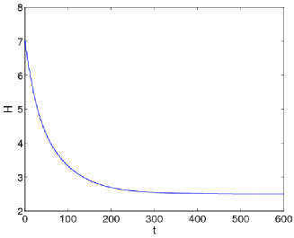
Figure 3: An unstable breather with frequency $a=0.9$, $\mathcal{PT}$-symmetry perturbation parameter $\epsilon=0.05$ and $\gamma(x)=x\exp[-(x/2)^{2}]$, initially centered at $x=0$ is displaced to $x_{0}=-2$ (left panels) or $x_{0}=2$ (right panels) and subsequently used as initial condition for a dynamical simulation. In the former case, the breather is inside the gain region and transforms through its increase of energy into a kink-antikink pair. In the latter case, the breather is located in the loss region and becomes mobile, while losing energy. The top left panel displays the evolution of the breather excitation $u(x,t)$ whereas the top right one, for the sake of better visualization, represents the energy density $E(x,t)$ of (14). The bottom panels show the evolution of the Hamiltonian energy of Eq. (14).

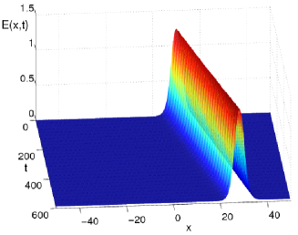
Figure 4: Same as Fig. 3 but for the breather displaced to $x_{0}=\pm 10$.

We have finally considered the evolution of unstable breathers located at $x_{0}=0$. If the breather is in the interval $\epsilon_{c,1}<\epsilon<\epsilon_{c,2}$, i.e. after the first bifurcation, the breather becomes quasi-periodic. For $\epsilon>\epsilon_{c,2}$ the breather transforms into a kink-antikink pair, similarly to the case of a breather located at the gain region. In both cases, the eigenvectors associated with the instabilities are localized in the gain ($x<0$) side. Fig. 5 shows two prototypical examples of these kinds of evolution. It is interesting to point out in this context that for this larger value of $\epsilon$, it can be seen that upon nucleation of the kink-antikink pair, the structure emerging on the gain side propagates unhindered, while the one appearing on the lossy side seems to decelerate and nearly stop. This is in line with earlier numerical (and semi-analytical) observations in Klein-Gordon models; cf. Ref. galley .

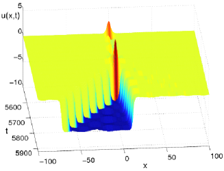
Figure 5: Dynamical evolution of an unstable breather with $\epsilon=0.1$ (left) and $\epsilon=0.18$ (right) located at $x_{0}=0$. Notice that in this figure and the previous ones, the points are taken with a rough time discretization that does not allow to observe the internal oscillation frequency $a$.

IV Conclusions & Future Challenges

In the present work, we have considered a prototypical example of the effect of $\mathcal{PT}$-symmetry on continuum breathers within the realm of the sine-Gordon equation. It has been shown through a Melnikov type calculation that the breathers are especially “delicate” persisting only at the special location of the interface between the gain and the loss. This non-robustness apparently renders these breathers linearly unstable, through a Hopf bifurcation as has been revealed in our Floquet analysis of the linearization problem and its monodromy matrix. Finally, the nonlinear dynamical evolution of the breathers has shown that when tilted towards the gain side, their energy grows until it is sufficient to nucleate a pair of a kink and anti-kink that subsequently separate from each other. On the other hand, in the case of the lossy side, it can be seen that the breathers gradually lose their energy, eventually being dissipated away.

Naturally many extensions of the present work can be considered. Perhaps the most natural one would be to explore the realm of discrete systems where breathers instead of being rather special, they are fairly generic macaub (under suitable non-resonance conditions). Understanding their persistence in such discrete settings might, in turn, reveal their potential observability in experimental settings (such as electrical lattices). Additionally, while here we have considered the special case of an exponentially decaying $\gamma(x)$ which corresponds purely to gain for $x<0$ and loss for $x>0$, it would be quite relevant to explore more complex forms of $\gamma(x)$, possibly involving oscillations of gain and loss (within the span of the breather) which may possess more complex breather existence and stability properties. Such studies are currently in progress and will be reported in future publications.

Appendix: Existence and stability of breathers

In order to perform a numerical analysis of the existence and stability of discrete breathers of frequency $a$ (which is in this case the natural parameter of the breather and assumes values $0<a<1$), we firstly need to discretize the spatial partial derivative in the sine-Gordon equation. We consider a finite-difference scheme so that

$$u_{xx}\approx\frac{1}{h^{2}}(u_{n+1}+u_{n-1}-2u_{n})$$ (15)

with $h$ being the discretization parameter. This transforms equation (1) into a set of $N$ coupled differential equations:

$$\ddot{u}_{n}+\epsilon\gamma(nh)\dot{u}_{n}+\sin u_{n}+\frac{1}{h^{2}}(u_{n+1}+u_{n-1}-2u_{n})=0$$ (16)

In order to calculate breathers in the $\mathcal{P}\mathcal{T}$-symmetric sine-Gordon model, we make use of a Fourier space implementation of the discretized dynamical equations (16) and continuations in frequency or gain/loss parameter are performed via a path-following (Newton-Raphson) method. Fourier space methods are based on the fact that the solutions are $T$-periodic, with $T=2\pi/a$; for a detailed explanation of these methods, the reader is referred to Refs. AMM99 ; Marin ; Cuevas . The method has the advantage, among others, of providing an explicit, analytical form of the Jacobian. Thus, the solution for the discretized system can be expressed in terms of a truncated Fourier series expansion:

$$u_{n}(t)=\sum_{k=-k_{m}}^{k_{m}}z_{k,n}\exp(\mathrm{i}kat)\ ,$$ (17)

with $k_{m}$ being the maximum of the absolute value of the running index $k$ in our Galerkin truncation of the full Fourier series solution. In the numerics, $k_{m}$ has been chosen as 15. After the introduction of (17), the equations (16) yield a set of $N\times(2k_{m}+1)$ nonlinear, coupled algebraic equations:

$$F_{k,n}\equiv-a^{2}k^{2}z_{k,n}-\mathrm{i}\gamma(nh)akz_{k,n}+{\cal F}_{k,n}-\frac{1}{h^{2}}(z_{k,n+1}+z_{k,n-1}-2z_{k,n})=0\ .$$ (18)

Here, ${\cal F}_{k,n}$ denotes the Discrete Fourier Transform:

$${\cal F}_{k,n}=\frac{1}{\cal N}\sum_{q=-k_{m}}^{k_{m}}\sin\left(\sum_{p=-k_{m}}^{k_{m}}z_{p}\exp\left[\mathrm{i}\frac{2\pi pn}{\cal N}\right]\right)\exp\left[-\mathrm{i}\frac{2\pi kq}{\cal N}\right],$$ (19)

with ${\cal N}=2k_{m}+1$. As $u_{n}(t)$ must be a real function, it implies that $z_{-k,n}=z^{*}_{k,n}$.

In order to study the spectral stability of periodic orbits, we introduce a small perturbation $\xi_{n}$ to a given solution $u_{n,0}$ of Eq. (16) according to $u_{n}=u_{n,0}+\xi_{n}$. Then, the equations satisfied to first order in $\xi_{n}$ read:

$$\ddot{\xi}_{n}+\cos(u_{0})\xi_{n}-\gamma(nh)\dot{\xi}_{n}-\frac{1}{h^{2}}(\xi_{n+1}+\xi_{n-1}-2\xi_{n})=0\ .$$ (20)

In order to study the spectral (linear) stability analysis of the relevant solution, a Floquet analysis can be performed if there exists $T\in\mathbb{R}$ so that the map $\{u_{n}(0)\}\rightarrow\{u_{n}(T)\}$ has a fixed point (which constitutes a periodic orbit of the original system). Then, the stability properties are given by the spectrum of the Floquet operator $\mathcal{M}$ (whose matrix representation is the monodromy) defined as:

$$\left(\begin{array}[]{c}\{\xi_{n}(T)\}\\ \{\dot{\xi}_{n}(T)\}\\ \end{array}\right)=\mathcal{M}\left(\begin{array}[]{c}\{\xi_{n}(0)\}\\ \{\dot{\xi}_{n}(0)\}\\ \end{array}\right).$$ (21)

The $2N\times 2N$ monodromy eigenvalues $\Lambda=\exp(\mathrm{i}\theta)$ are dubbed the Floquet multipliers and $\theta$ are denoted as Floquet exponents (FEs). This operator is real, which implies that there is always a pair of multipliers at $1$ (corresponding to the so-called phase and growth modes Marin ; Cuevas ) and that the eigenvalues come in pairs $\{\Lambda,\Lambda^{*}\}$.

References

- (1) C.M. Bender and S. Boettcher, Phys. Rev. Lett. 80, 5243 (1998).
- (2) C.M. Bender, S. Boettcher, and P.N. Meisinger, J. Math. Phys. 40, 2201 (1999)
- (3) C. M. Bender, Rep. Prog. Phys. 70 (2007) 947–1018.
- (4) A. Ruschhaupt, F. Delgado, and J.G. Muga, J. Phys. A: Math. Gen. 38 (2005) L171–L176.
- (5) Z. H. Musslimani, K. G. Makris, R. El-Ganainy, and D. N. Christodoulides, Phys. Rev. Lett. 100 (2008) 030402 (4 pages).
- (6) H. Ramezani, T. Kottos, R. El-Ganainy, and D.N. Christodoulides, Phys. Rev. A 82 (2010), 043803 (6 pages).
- (7) A. Guo, G.J. Salamo, D. Duchesne, R. Morandotti, M. Volatier-Ravat, V. Aimez, G. A. Siviloglou, and D. N. Christodoulides, Phys. Rev. Lett. 103, 093902 (2009).
- (8) C.E. Rüter, K.G. Makris, R. El-Ganainy, D.N. Christodoulides, M.Segev, and D. Kip, Nature Physics 6 (2010) 192–195.
- (9) B. Peng, S.K. Ozdemir, F. Lei, F. Monifi, M. Gianfreda, G.L. Long, S. Fan, F. Nori, C.M. Bender, L. Yang, Nature Physics 10 (2014) 394 -398.
- (10) C.M. Bender, B.J. Berntson, D. Parker and E. Samuel, Am. J. Phys. 81, 173 (2013).
- (11) J. Schindler, A. Li, M. C. Zheng, F. M. Ellis, and T. Kottos, Phys. Rev. A 84, 040101 (2011).
- (12) H. Ramezani, J. Schindler, F. M. Ellis, U. Günther, and T. Kottos, Phys. Rev. A 85, 062122 (2012).
- (13) F.Kh. Abdullaev, Y.V. Kartashov, V.V. Konotop, and D.A. Zezyulin, Phys. Rev. A 83, 041805(R) (2011).
- (14) N. V. Alexeeva, I. V. Barashenkov, A.A. Sukhorukov, and Yu.S. Kivshar, Phys. Rev. A 85, 063837 (2012)
- (15) I.V. Barashenkov, S.V. Suchkov, A.A. Sukhorukov, S.V. Dmitriev and Yu.S. Kivshar, Phys. Rev. A 86, 053809 (2012)
- (16) R. Driben and B.A. Malomed, Opt. Lett. 36, 4323 (2011).
- (17) R. Driben and B.A. Malomed, EPL 96, 51001 (2011).
- (18) S. Nixon, L. Ge, and J. Yang, Phys. Rev. A 85, 023822 (2012).
- (19) S.V. Dmitriev, A.A. Sukhorukov, and Yu.S. Kivshar, Opt. Lett. 35, 2976 (2010).
- (20) V.V. Konotop, D.E. Pelinovsky, and D.A. Zezyulin, EPL 100, 56006 (2012).
- (21) A.A. Sukhorukov, S.V. Dmitriev, S.V. Suchkov, and Yu.S. Kivshar, Opt. Lett. 37, 2148 (2012).
- (22) Yu.V. Bludov, R. Driben, V.V. Konotop, B.A. Malomed, J. Opt. 15, 064010 (2013).
- (23) J. Yang, Phys. Lett. A 378, 367–373 (2014) and also J. Yang, Opt. Lett. 39, 1133-1136 (2014).
- (24) K. Li and P.G. Kevrekidis, Phys. Rev. E 83, 066608 (2011).
- (25) K. Li, P.G. Kevrekidis, B.A. Malomed, and U. Günther, J. Phys. A Math. Theor. 45, 444021 (2012)
- (26) S.V. Suchkov, B.A. Malomed, S.V. Dmitriev and Yu.S. Kivshar, Phys. Rev. E 84, 046609 (2011).
- (27) A.A. Sukhorukov, Z. Xu, and Yu.S. Kivshar, Phys. Rev. A 82, 043818 (2010).
- (28) D.A. Zezyulin and V.V. Konotop, Phys. Rev. Lett. 108, 213906 (2012).
- (29) N. V. Alexeeva, I. V. Barashenkov, K. Rayanov, S. Flach, arXiv:1308.5862.
- (30) I. V. Barashenkov, G.S Jackson, S. Flach, Phys. Rev. A 88, 053817 (2013).
- (31) N. Lazarides and G. P. Tsironis, Phys. Rev. Lett. 110, 053901 (2013).
- (32) J. Cuevas, P.G. Kevrekidis, A. Saxena and A. Khare, Phys. Rev. A 88, 032108 (2013).
- (33) A. Demirkaya, D. J. Frantzeskakis, P. G. Kevrekidis A. Saxena, and A. Stefanov, Phys. Rev. E 88, 023203 (2013).
- (34) A. Demirkaya, M. Stanislavova, A. Stefanov, T. Kapitula and P.G. Kevrekidis, arXiv:1402.2942.
- (35) I.V. Barashenkov and M. Gianfreda, J. Phys. A: Math. Theor. 47 282001 (2014).
- (36) N. Bender, S. Factor, J. D. Bodyfelt, H. Ramezani, D. N. Christodoulides, F. M. Ellis, and T. Kottos, Phys. Rev. Lett. 110, 234101 (2013).
- (37) B. Birnir, H.P. McKean and A. Weinstein, Comm. Pure Appl. Math. 47, 1043 (1994).
- (38) J. Denzler, Comm. Math. Phys. 158, 397 (1993).
- (39) J. Shatah, C.C. Zeng, Nonlinearity 16, 591 (2003).
- (40) N. Lu, J. Differ. Equations 256, 745 (2014).
- (41) J. Guggenheimer, P. Holmes, Nonlinear Oscillations, Dynamical Systems and Bifurcation of Vector Fields, Springer-Verlag (New York, 1983).
- (42) S. Aubry, Physica D 103, 201 (1997).
- (43) S. Flach and A. V. Gorbach, Phys. Rep. 467, 1 (2008).
- (44) J.F.R. Archilla, R.S. MacKay, and J.L. Marín, Physica D 134, 406 (1999).
- (45) J.L. Marín, Intrinsic Localized Modes in nonlinear lattices. PhD Thesis, University of Zaragoza (1999).
- (46) J. Cuevas Localization and energy transfer in anharmonic inhomogeneus lattices PhD Thesis, University of Sevilla (2003).
- (47) R.K. Dodd, J.C. Eilbeck, J.D. Gibbon and H.C. Morris, Solitons and Nonlinear Wave Equations, Academic Press (London, 1982).
- (48) P.G. Kevrekidis, Phys. Rev. A 89, 010102(R) (2014).
- (49) R.S. MacKay and S. Aubry, Nonlinearity 7, 1623 (1994).