Strongly bound yet light bipolarons for double-well electron-phonon coupling

Abstract

We use the Momentum Average approximation (MA) to study the ground-state properties of strongly bound bipolarons in the double-well electron-phonon (el-ph) coupling model, which describes certain intercalated lattices where the linear term in the el-ph coupling vanishes due to symmetry. We show that this model predicts the existence of strongly bound yet lightweight bipolarons in some regions of the parameter space. This provides a novel mechanism for the appearance of such bipolarons, in addition to long-range el-ph coupling and special lattice geometries.

I Introduction

The coupling of charge carriers to lattice degrees of freedom (phonons) plays an important role in determining the properties of a wide range of materials such as organic semiconductors,Matsui et al. (2010); Ciuchi and Fratini (2011) cuprates,Lanzara et al. (2001); Shen et al. (2004); Reznik et al. (2006); Lee et al. (2006); Gadermaier et al. (2010); Gunnarsson and Rösch (2008) manganites,Mannella et al. (2005) two-gap superconductors like MgB₂,Yildirim et al. (2001); Liu et al. (2001); Mazin and Antropov (2003); Choi et al. (2002) and many more.

When a charge carrier becomes dressed by a cloud of phonons, the quasi-particle that forms – the polaron – may have quite different properties from the free particle, such as a larger effective mass and renormalized interactions with other particles. One particularly interesting effect of the latter is the formation of bipolarons, where an effective attraction mediated by exchange of phonons binds the carriers together. If the binding is strong enough, the two phonon clouds merge into one, resulting in a so-called S0 bipolaron. Weaker binding, where each polaron maintains its cloud and the binding is mediated by virtual visits to the other carrier’s cloud, is also possible and results in a S1 bipolaron.Bonc̆a et al. (2000); macridin

The existence of bipolarons is interesting for many reasons. For instance, it has been suggested that Bose-Einstein condensation of bipolarons might be responsible for superconductivity in some high-$T_{c}$ materials.*[See][foranoverview.]alexandrov_review For this to occur, the bipolaron must be strongly bound so it can survive up to high temperatures. However, such strong binding generally requires strong electron-phonon coupling. In most simple models of el-ph coupling such as the Holstein model,Holstein (1959) this also results in a large effective mass of the bipolaronBonc̆a et al. (2000); macridin which severely reduces its mobility and makes it likely to become localized by even small amounts of disorder.

For this reason, much of the theoretical work on bipolarons is focused on finding models and parameter regimes for which the bipolaron is strongly bound yet relatively light. So far, successful mechanism are based either on longer-range electron-phonon interactionsBonča and Trugman (2001); Hague et al. (2007); Alexandrov et al. (2012); daven or on special lattice geometries such as one-dimensional ladders or triangular lattices.Hague and Kornilovitch (2010)

Here we show that the recently proposed (short-range) double-well el-ph coupling modelAdolphs and Berciu (2014) also predicts the existence of strongly bound bipolarons with relatively low effective mass in certain regions of the parameter space, thus revealing another possible mechanism for their appearance. Our study uses the Momentum Average (MA) approximation,Berciu (2006); Goodvin et al. (2006); Adolphs and Berciu (2013, 2014) which we validate with exact diagonalization in an enlarged variational space. Since in the single-particle case the dimensionality of the underlying lattice had little qualitative impact, we focus here on the one-dimensional case.

This work is organized as follows. In Section II we introduce the Hamiltonian for the double-well model and in Section III we discuss the methods we use to solve it. In Section IV we present results for the bipolaron binding energy and effective mass, and in Section V we summarize our conclusions and an outlook for future work.

II Model

The double-well el-ph coupling model was introduced in Ref. Adolphs and Berciu, 2014 for the single polaron case. For ease of reference, we repeat some of its motivation and introduction here.

The model is relevant for crystals whose structure is such that a sublattice of light ions is symmetrically intercalated with one of much heavier ions; the latter are assumed to be immobile. Moreover, charge transport occurs on the sublattice of the light ions. An example is the one-dimensional intercalated chain shown in Fig. 1(a). Another example is a two-dimensional CuO layer, sketched in Fig. 1(b), where the doping holes move on the light oxygen ions placed in between the heavy copper ions. In such structures, because in equilibrium each light ions is symmetrically placed between two immobile heavy ions, the potential felt by a carrier located on a light ion must be an even function of that ion’s longitudinal displacement from equilibrium, i.e. the first derivative of the local potential must vanish. As a result, the linear electron-phonon coupling is zero by symmetry, and one needs to consider the quadratic coupling. This is what the double-well el-ph coupling model does.

Starting from the single-polaron Hamiltonian describing double-well el-ph coupling, introduced in Ref. Adolphs and Berciu, 2014, we add the appropriate terms for the many-electron problem to obtain

$$\mathcal{H}=\hat{T}+\Omega\sum_{i}b_{i}^{\dagger}b_{i}^{\phantom{\dagger}}+U\sum_{i}\hat{n}_{i\uparrow}\hat{n}_{i\downarrow}\\ +g_{2}\sum_{i\sigma}c_{i\sigma}^{\dagger}c_{i\sigma}^{\phantom{\dagger}}\left(b_{i}^{\dagger}+b_{i}^{\phantom{\dagger}}\right)^{2}+\sum_{i}g_{4}^{n_{i}}\left(b_{i}^{\dagger}+b_{i}^{\phantom{\dagger}}\right)^{4}.$$ (1)

Here, $c_{i\sigma}$ and $b_{i}$ are annihilation operators for a spin-$\sigma$ carrier at site $i$, and a phonon at site $i$. $\hat{T}$ describes hopping of free carriers on the sublattice of light ions in an intercalated lattice like that sketched in Fig. 1. For simplicity, we consider nearest-neighbor hopping only, $\hat{T}=-t\sum_{\langle i,j\rangle,\sigma}c_{i\sigma}^{\dagger}c_{j\sigma}^{\phantom{\dagger}}+h.c.$, although our method can also treat longer-range finite hopping.Möller et al. (2012) The next two terms describe a single branch of dispersionless optical phonons with energy $\Omega$, and the Hubbard on-site Coulomb repulsion with strength $U$. The last two terms describe the el-ph coupling in the double-well model. As mentioned, in lattices like that sketched in Fig. 1, the coupling depends only on even powers of the light-ion displacement $\delta\hat{x}_{i}\propto b_{i}^{\dagger}+b_{i}$ (the heavy ions are assumed to be immobile). As a result, the lowest order el-ph coupling is the quadratic term whose characteristic energy $g_{2}$ can have either sign, depending on modeling details. As discussed at length in Ref. Adolphs and Berciu, 2014, the interesting physics occurs when $g_{2}<0$ so that the el-ph coupling “softens” the lattice potential. For sufficiently negative $g_{2}$ this renders the lattice locally unstable in the harmonic approximation and requires the inclusion of quartic terms in the lattice potential. For consistency, one should then also include quartic terms in the el-ph coupling. As detailed in Ref. Adolphs and Berciu, 2014, under reasonable assumptions the quartic lattice terms can be combined with the quartic el-ph coupling term on sites hosting a carrier and ignored on all other sites. Because the resulting quartic term contains contributions from both the lattice potential and from the el-ph interaction, it should not be assumed to be linear in the carrier number, unlike the quadratic term which arises purely from el-ph coupling. Instead, we use the general form

$$g_{4}^{(n_{i})}=g_{4}\cdot\begin{cases}0,&\mbox{ if }n_{i}=0\\ 1,&\mbox{ if }n_{i}=1\\ \alpha,&\mbox{ if }n_{i}=2\end{cases}$$

where $n_{i}=\sum_{\sigma}c^{\dagger}_{i\sigma}c_{i\sigma}$ is the number of carriers on site $i$, and $\alpha$ is a constant between $1$ and $2$. Setting $\alpha=2$ assumes that quartic lattice effects are negligible compared to the quartic el-ph terms, whereas $\alpha=1$ is the opposite extreme. For the remainder of this article we set $\alpha=1$, so that $g_{4}^{(1)}=g_{4}^{(2)}=g_{4}$. This case leads to stronger coupling, since a lower $g_{4}$ results in deeper wells that are further apart,Adolphs and Berciu (2014) and thus represents the parameter regime we are interested in. Physically, this describes the situation where the quartic lattice terms are much larger than the quartic el-ph coupling; however they are still negligible compared to the quadratic lattice terms and therefore can be ignored at sites without a carrier.

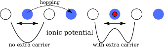
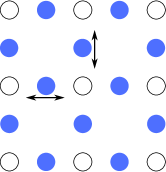
Figure 1: (color online) Sketch of the crystal structures dis- cussed in this work: (a) 1D chain, and (b) 2D plane, consist- ing of light atoms (filled circles) intercalated between heavy atoms (empty circles). In the absence of carriers, the ionic potential of a light atom is a simple harmonic well. In the presence of a carrier, the ionic potential of the light atom hosting it remains an even function of its longitudinal dis- placement, so the linear e-ph coupling vanishes. In suitable conditions the effective ionic potential becomes a double well. (Reproduced from Ref. Adolphs and Berciu, 2014)

III Formalism

We compute the bipolaron binding energy and effective mass using the momentum average (MA) approximation.Berciu (2006); Goodvin et al. (2006); Adolphs and Berciu (2013, 2014) Since we are interested in strongly-bound bipolarons which have a large probability of having both carriers on the same site, the version of MA used here is the variational approximation that discounts states where the two carriers occupy different sites. This results in an analytic expression of the two-particle Green’s function which is used to efficiently explore the whole parameter space. The accuracy of this flavor of MA is verified by performing exact diagonalization in a much larger variational subspace (details are provided below). In the regime of interest the agreement is very favorable, showing that the effort required to perform the analytical calculation for a flavor of MA describing a bigger variational space is not warranted.

III.1 Momentum Average approximation

We define states with both carriers at the same site, $|{i}\rangle=c_{i\uparrow}^{\dagger}c_{i\downarrow}^{\dagger}|{0}\rangle$, and states of given total momentum $\vec{k}$ with both carriers at the same site,

$$|{\vec{k}}\rangle=\frac{1}{\sqrt{N}}\sum_{i}e^{i\vec{k}\cdot\vec{r}_{i}}|{i}\rangle.$$

The bipolaron dispersion $E_{\text{bp}}(\vec{k})$ is obtained from the lowest energy pole of the two-particle Green’s function

$$G(\vec{k},\omega)=\langle{\vec{k}|[\omega-\mathcal{H}+i\eta]^{-1}|\vec{k}}\rangle,$$

where $\eta\rightarrow 0^{+}$ is a small convergence factor. The effective bipolaron mass is $1/m_{\text{bp}}=\partial^{2}E_{\text{bp}}/\partial k^{2}|_{k=0}$. Throughout this work we set $\hbar=1,a=1$.

We split the Hamiltonian into $\mathcal{H}=\mathcal{H}_{0}+\mathcal{H}_{1}$ with $\mathcal{H}_{0}=\hat{T}+\Omega\sum_{i}b_{i}^{\dagger}b_{i}$ describing the free system and $\mathcal{H}_{1}$ containing the interaction terms. We apply Dyson’s identity $\hat{G}(\omega)=\hat{G}_{0}(\omega)+\hat{G}(\omega)\mathcal{H}_{1}\hat{G}_{0}(\omega)$ where

$$\hat{G}_{0}(\omega)=\left[\omega-\mathcal{H}_{0}+i\eta\right]^{-1}$$

is the resolvent of $\mathcal{H}_{0}$ and we also define

$$G_{0}(\vec{k},\omega)=\langle{\vec{k}|\hat{G}_{0}(\omega)|\vec{k}}\rangle=\frac{1}{N}\sum_{\vec{q}}\frac{1}{\omega+i\eta-\epsilon(\vec{k}-\vec{q})-\epsilon(\vec{q})}$$

as a non-interacting two-particle propagator, where $\epsilon(\vec{k})$ is the free carrier dispersion. $N\rightarrow\infty$ is the number of light-ion sites of the lattice. In 1D, $G_{0}(\vec{k},\omega)$ equals the momentum-averaged single-particle free propagator in one dimension for an effective hopping integral $2t\cos(k/2)$, for which an analytic expression is known.Economou In higher dimensions, such propagators can be calculated as discussed in Ref. few_particle, .

As mentioned, in a variational sense the MA used here amounts to neglecting all states where the carriers are not on the same site. This approximation is justified for the description of the strongly bound on-site (S0) bipolaron, which is expected to have most of its weight in the sector where both carriers are on the same site. Another way to look at this is that the bipolaron ground-state energy in the strongly-bound case must be well below the non-interacting two-particle continuum, and the free two-particle propagator will have vanishingly small off-diagonal matrix elements at such energies. Ignoring them, the equation of motion becomes $G(\vec{k},\omega)\approx G_{0}(\vec{k},\omega)+\langle{\vec{k}|\hat{G}(\omega)\mathcal{H}_{1}|\vec{k}}\rangle G_{0}(\vec{k},\omega)$, and thus:

$$G(\vec{k},\omega)=G_{0}(\vec{k},\omega)\left(1+\sum_{i}\frac{e^{ikR_{i}}}{\sqrt{N}}\left[(g_{2}+6g_{4})F_{1}(\vec{k},\omega,i)\\ +g_{4}F_{2}(\vec{k},\omega,i)+UF_{0}(\vec{k},\omega,i)\right]\right).$$

where $F_{n}(\vec{k},\omega,i)=\langle{\vec{k}|\hat{G}(\omega)b_{i}^{\dagger,2n}|i}\rangle$ is a generalized two-particle propagator. Equations of motion for the $F_{n}$ propagators are obtained in the same way, and read:

$$F_{n}(\vec{k},\omega,i)=\bar{g}_{0}(\omega-2n\Omega)\Big{[}g_{4}(2n)^{\bar{4}}F_{n-2}(\vec{k},\omega,i)\\ +\big{(}(2g_{2}+6g_{4})(2n)^{\bar{2}}+4g_{4}(2n)^{\bar{3}}\big{)}F_{n-1}(\vec{k},\omega,i)\\ +(8ng_{2}+12ng_{4}+24n^{2}g_{4}+U)F_{n}(\vec{k},\omega,i)\\ +(2g_{2}+6g_{4}+8ng_{4})F_{n+1}(\vec{k},\omega,i)+g_{4}F_{n+2}(\vec{k},\omega,i)\Big{]}.$$ (2)

where we use the shorthand notation $x^{\bar{n}}=x!/(x-n)!$ and have introduced the momentum-averaged free two-carrier propagator,

$$\bar{g}_{0}(\omega):=\langle{i|\hat{G}_{0}(\omega)|i}\rangle=\frac{1}{N}\sum_{\vec{k}}G_{0}(\vec{k},\omega)\\ =\frac{1}{N^{2}}\sum_{\vec{k},\vec{q}}\frac{1}{\omega-\epsilon(\vec{k}-\vec{q})-\epsilon(\vec{q})+i\eta}.$$

In 1D, $\bar{g}_{0}(\omega)$ equals the diagonal element of the free propagator for a particle in 2D, which can be expressed in terms of elliptical functions and calculated efficiently.Economou Similar considerations hold in higher dimensions.few_particle

The equations of motions are then solved following the procedure described at length in Refs. Adolphs and Berciu, 2014, 2013. For consistency, we sketch the main steps here. First, we introduce vectors $W_{n}=(F_{2n-1},F_{2n})^{T}$ for $n\geq 0$ (the arguments $\vec{k},\omega,i$ of the propagators are not written explicitly from now on). Note that with this definition, $W_{0}=(F_{-1},F_{0})$, yet $F_{-1}$ is not properly defined. However, the final result has no dependence on $F_{-1}$, as we show below. The equations of motion are then rewritten in terms of $W_{n}$ to read $\gamma_{n}W_{n}=\alpha_{n}W_{n-1}+\beta_{n}W_{n+1}$. The matrix elements of the $2\times 2$ matrices $\alpha_{n},\beta_{n},\gamma_{n}$, are easily read off Eq. (2).

Defining $A_{n}=[\gamma_{n}-\beta_{n}A_{n+1}]^{-1}\alpha_{n}$, the physical solution of these recurrence equations is $W_{n}=A_{n}W_{n-1}$. Introducing a sufficiently large cut-off $N_{c}$ where $W_{N_{c}}=0$, we can then compute $A_{1}$ and have $W_{1}=A_{1}W_{0}$, i.e.,

$$\begin{pmatrix}F_{1}\\ F_{2}\end{pmatrix}=A_{1}\begin{pmatrix}F_{-1}\\ F_{0}\end{pmatrix}=\begin{pmatrix}a_{11}&a_{12}\\ a_{21}&a_{22}\end{pmatrix}\begin{pmatrix}F_{-1}\\ F_{0}\end{pmatrix}.$$

One can easily check that $a_{11}=a_{21}=0$. Thus, we obtain $F_{1}=a_{12}F_{0}$ and $F_{2}=a_{22}F_{0}$. Substituting these results back into the EOM for $G$ we obtain

$$G(\vec{k},\omega)=G_{0}(\vec{k},\omega)\Big{[}1+\\ \sum_{i}\frac{e^{i\vec{k}\vec{R}_{i}}}{\sqrt{N}}\left((2g_{2}+6g_{4})a_{12}+g_{4}a_{22}+U\right)F_{0}(\vec{k},\omega,i)\Big{]}.$$

Since, by definition, $G(\vec{k},\omega)=\sum_{i}\frac{e^{i\vec{k}\vec{R}_{i}}}{\sqrt{N}}F_{0}(\vec{k},\omega,i)$, and given that $a_{12},a_{22}$ are functions of $\omega$ only, we find:

$$G(\vec{k},\omega)=\frac{1}{G_{0}^{-1}(\vec{k},\omega)-(2g_{2}+6g_{4})a_{12}-g_{4}a_{22}-U}.$$ (3)

Note that the coefficients $a_{12}$ and $a_{22}$ depend on all parameters of the model, including $U$. As a result, the position of the lowest pole of Eq. (3) is not simply linear in $U$, although this is a good approximation for the strongly bound bipolaron.

We emphasize that this MA expression becomes exact in two limiting cases. First, in the atomic limit $t\rightarrow 0$ the free propagator has no off-diagonal terms and thus no error is introduced by dropping them from the equations of motion. Second, without el-ph interactions ($g_{n}=0$) the Hamiltonian reduces to the Hubbard model which is exactly solvable in the two-particle case.Sawatzky (1977) In both cases MA gives the exact solution.

III.2 Exact Diagonalization

The results obtained via MA as outlined above are checked against exact diagonalization results in a bigger variational subspace designed to describe well the strongly bound S0 bipolaron. Hence, we only consider states where all the phonons are located on the same lattice site and at least one of the two electrons is close to this cloud. The basis states are of the form

$$|{\vec{k},n,\delta_{1},\delta_{2}}\rangle=\sum_{i}\frac{e^{i\vec{k}\vec{r}_{i}}}{\sqrt{N}}b_{i}^{\dagger,n}c_{i+\delta_{1},\uparrow}^{\dagger}c_{i+\delta_{2},\downarrow}^{\dagger}|{0}\rangle$$

with the constraint that either $\delta_{1}$ or $\delta_{2}$ is below a certain cut-off. In addition, a global cut-off $N_{c}$ is imposed on $n+\delta_{1}+\delta_{2}$. The ground state within the variational space is then computed using standard eigenvalue techniques.

The main difference between these ED and MA results is that MA discards contributions from configurations where the carriers are at different lattice sites. Comparing the two therefore allows us to gauge the importance of such terms, and to decide whether the speed gained from using the analytical MA expressions counterbalances the loss of accuracy.

IV Results

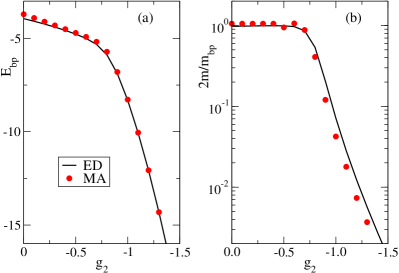
Figure 2: (color online) (a) Bipolaron ground-state energy, and (b) inverse effective mass for $t=1,\Omega=0.5$, $g_{4}=0.1$, computed with ED (solid black line) and MA (red dots).

From now on we focus on the one-dimensional (1D) case, since our previous workAdolphs and Berciu (2014) suggests that going to higher dimensions leads to qualitatively similar results.

Before discussing the MA results, we first compare them to those obtained from ED in the larger variational subspace discussed above. A typical comparison (for $t=1,\Omega=0.5$ and $g_{4}=0.1$) is shown in Fig. 2. The left panel shows the ground state energy and the right panel shows the inverse effective mass of the bipolaron. In the regime where the bipolaron is strongly bound, i.e. where its energy decreases fast and its effective mass increases sharply as $|g_{2}|$ increases, we find excellent agreement for the energy. The masses also agree reasonably well, but MA systematically overestimates the bipolaron mass. This is a direct result of the more restrictive nature of the MA approximation: By discarding configurations where the carriers occupy different sites, the mobility of the bipolaron is underestimated and thus the effective mass is overestimated. Nonetheless, this error is not very large, and only means that the bipolarons in the double well model are even lighter than calculated by MA. Due to similarly good agreement in all cases we verified, for the remainder of this work we only discuss results obtained with the more efficient MA method.

We emphasize that our approximation for computing the Green’s function is only valid in the regime of strong binding and does not describe correctly the physics at weak coupling. Since neither MA nor ED, as implemented here, allow for the formation of two phonon clouds, neither describes the formation of a weakly bound S1 bipolaron (where polarons form on neighboring sites and interact with each other’s clouds via virtual hoppings), nor the dissociation into two polarons as the coupling is further decreased.Bonc̆a et al. (2000); macridin Accuracy in these parameter regimes can be improved by applying more sophisticated – yet much more tedious – versions of MA or ED for suitably expanded variational spaces. For the purpose of this work, however, we want to focus on the strong-coupling regime, where our results are accurate.

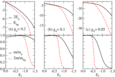
Figure 3: (color online) Ground-state properties (total energy and inverse mass) of the S0 bipolaron and two independent polarons for $t=1,\Omega=0.5$ and $g_{4}=0.2$, $0.1$, and $0.05$ for a), b), and c), respectively. For all panels, $U=0$.

We show the ground-state properties of the bipolaron compared to those of two single polarons in Figs. 3, 4 for two different values of $\Omega$. In all those panels, we have set $U=0$ for simplicity; the role of finite $U$ will be discussed at the end of this section.

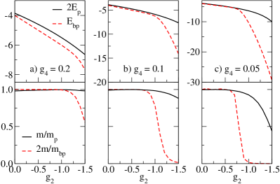
Figure 4: (color online) Ground-state properties (total energy and inverse mass) of the S0 bipolaron and two independent polarons for $t=1,\Omega=2$ and $g_{4}=0.2$, $0.1$, and $0.05$ for a), b), and c), respectively. For all panels, $U=0$.

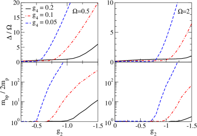
Figure 5: (color online) Binding energy $\Delta$ and effective-mass ratio $m_{\rm bp}/2m_{\rm p}$ of the bipolarons for $\Omega=0.5$ and $\Omega=2$ at different values of $g_{4}$.

The ground state energy of the bipolaron behaves qualitatively similar for all values of $\Omega$ and $g_{4}$ in that it shows a kink at some $g_{2}$ where the slope becomes steeper. This signifies the onset of the strong-coupling regime where the bipolaron energy is well below the energy of two independent polarons, consistent with a strongly bound bipolaron. At weaker coupling the results are not accurate since – as explained above – our version of MA cannot describe the dissociation of the bipolaron.

Consider now the behavior of the effective masses. For all parameters considered here, we see that the single polaron mass $m_{p}$ starts out slightly above the free electron mass $m$, then decreases until it is almost as light as the free electron, before increasing again. This turnaround in the polaron mass is due to partial cancellation effects of the quadratic and quartic el-ph coupling terms, as discussed in Ref. Adolphs and Berciu, 2014. We observe that when the bipolaron is already quite strongly bound, the single polaron can still be very light. Empirically, we find that in the strong-coupling regime $m_{\rm p}\sim m\exp(-\gamma\Delta_{\rm p}/\Omega)$ where $\Delta_{\rm p}=-2t-E_{\rm p}$ is the single-polaron binding energy and $\gamma$ is a small numerical prefactor. This behavior is also found in the Holstein modelHolstein (1959) in the strong-coupling limit, where $\gamma=1,\Delta_{\rm p}=-g^{2}/\Omega$. The prefactor $\gamma$ can be much smaller in the double well model because of the nature of the ionic potential. This was explained in detail in Ref. Adolphs and Berciu, 2014, and will be discussed in the context of bipolarons later in this section.

The bipolaron effective mass fluctuates around the value of $2m$ in the weak coupling regime. As explained above, here our method does not describe two independent polarons, but two independent free electrons whose effective mass should just be $2m$. However, the two-particle spectral function in this case does not have a low-energy quasi-particle peak. Instead, it has a continuum spanning the allowed two-particle continuum.

These issues disappear at stronger coupling where a strongly bound bipolaron forms and MA becomes accurate. The figures show that here the bipolaron quickly gains mass with increased coupling strength $|g_{2}|$, and that this increase is stronger the smaller $g_{4}$ is. Note that a smaller $g_{4}$ actually means stronger coupling, because the wells are deeper and further apart.Adolphs and Berciu (2014)

The same data is displayed in a different way in Fig. 5, where we show the magnitude of the bipolaron binding energy $\Delta=2E_{\rm p}-E_{\rm bp}$ and the ratio of bipolaron to single-polaron masses, $m_{\rm bp}/2m_{\rm p}$. The strongly bound bipolaron regime (where the results are accurate) is reached when these quantities vary fast with $g_{2}$. In particular, the results for $m_{\rm bp}/2m_{\rm p}$ show that here the bipolaron mass increases much more quickly than the polaron mass. This is not surprising for models like this, where the phonons modulate the on-site energy of the carrier. At strong coupling the results can be understood starting from the atomic limit $t=0$, treating hopping as a perturbation. Since both carriers must hop in order for the bipolaron to move, one expects that $m_{\rm bp}/m\propto(m_{\rm p}/m)^{2}$; indeed, we find this relation to be valid for a wide range of parameters for our model.

Although in this regime the bipolaron quickly gains mass, there are parameter ranges where its mass is still rather light while the bipolaron is strongly bound. Examples of such parameters are given in Table 1. We note that qualifiers such as ”strongly bound“ and ”light“ are subjective. In our case, we take the bipolaron as strongly bound when the binding energy $\Delta/\Omega>1$ and the ratio $m_{\rm bp}/2m<10-20$, consistent with other references.Hague and Kornilovitch (2010); Bonča and Trugman (2001)

Table 1: Some example values of the bipolaron binding energy and effective mass.

$\Omega$	$g_{4}$	$|g_{2}|$	$\Delta/t$	$m^{**}/2m$
$0.5$	$0.1$	0.9	1.25	8.3
	$0.2$	1.3	1.48	4.4
$2$	$0.1$	1.3	3.11	5.9
	$0.2$	1.5	1.03	1.8

Light but strongly bound bipolarons were previously found for long-range el-ph coupling.Bonča and Trugman (2001) The explanation is that in such models, carriers induce a spatially extended lattice deformation, not one that is located in the immediate vicinity of the carrier as is the case at strong coupling in local el-ph coupling models. Because of their extended nature, the overlap between clouds displaced by one lattice site (which controls the effective hopping) remains rather large, meaning that the polarons and bipolarons remain rather light in such models.

Even though it is due to a local el-ph coupling, the mechanism resulting in light bipolarons in our model is qualitatively similar, as illustrated in Fig. 6. In the linear Holstein model the effect of an additional carrier added to a lattice site is to shift the equilibrium position of the ionic potential. The ionic wavefunctions corresponding to an empty and an occupied site therefore have only small overlap, which strongly reduces the effective carrier hopping. In the double-well model, in contrast, the ionic wavefunction for the doubly-occupied site has appreciable overlap with the ionic wavefunction for an empty or a singly-occupied site and thus does not reduce the effective hopping as much.

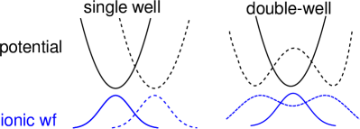
Figure 6: (color online) Ionic potential (above) and ionic ground-state wavefunction (below) in the single-well and double-well models. Solid lines correspond to the situation without an additional carrier, dashed lines to the situation with an additional carrier.

We conclude with a brief discussion of the effects of a finite, repulsive $U$. For a very strongly coupled S0 bipolaron, most of the weight is in states with both carriers on the same site. In this regime, the binding energy decreases (nearly) linearly with $U$, $\Delta_{\rm bp}(U)\approx\Delta_{\rm bp}(U=0)-U$. However, increasing $U$ increases the energy cost of the S0 state and thus encourages hybridization with off-site states, which results in an overall smaller effective mass. We show results for the bipolaron energy and effective mass as a function of $U$ in Fig. 7. We stay within the regime $U<\Delta_{\rm bp}$ where the bipolaron remains strongly bound. As predicted, the energy of the bipolaron increases linearly with $U$, which in turn means that the binding energy $\Delta_{\rm bp}$ decreases linearly with $U$. The effective mass also decreases (approximately) linearly with $U$. This can be demonstrated for the strong coupling limit via second order perturbation theory in the hopping. Following along the lines in Refs. Bonc̆a et al., 2000; macridin, , the effective hopping of the S0 bipolaron is of the form

$$m^{-1}_{\rm bp}\propto t_{\rm eff}\sim\frac{-t^{2}e^{-\gamma\Delta/\Omega}}{2E_{p}-U}$$

for some constant $\gamma$. We see that the mass itself decreases linearly with $U$, with a steeper slope the larger the effective mass at $U=0$.

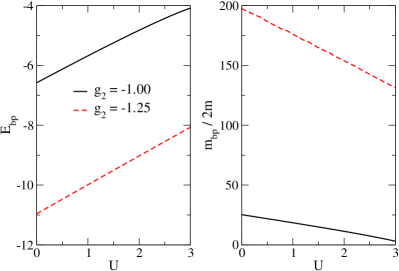
Figure 7: (color online) Bipolaron energy (left) and effective mass (right) as a function of the Hubbard $U$, for $t=1,\Omega=0.4$ and $g_{4}=0.1$. Similar results are found for other parameters if $U$ is not large enough to lead to bipolaron dissociation.

In essence, provided that it is not large enough to break the bonding, a finite $U$ does not change the overall picture and merely tunes the balance between the bipolaron binding energy and its effective mass.

V Conclusions and Outlook

In conclusion, we have investigated the bipolaron ground-state properties in the dilute limit of the double-well el-ph coupling model at strong coupling. We have demonstrated that due to the particular nature of the carrier-induced ionic potential, the double-well bipolaron can be strongly bound while remaining light compared to the bipolaron in the Hubbard-Holstein model. This suggests a new route to stabilizing such bipolarons, in addition to previously discussed mechanisms based on long-range el-ph coupling or special lattice geometries. We expect that a combination of these mechanisms will lead to even lighter bipolarons.

In this work, we have used and validated a simple extension of the Momentum Average approximation to the two-carrier case. While this generalization is appropriate to describe a strongly bound S0 bipolaron, it cannot describe the off-site (S1) bipolaron that forms at larger Hubbard repulsion $U$, or the unbinding of the bipolaron at even larger $U$. A more sophisticated version of MA, currently under development, will give us insight into the full phase diagram of the double-well model.