“Mental Rotation” by Optimizing
Transforming Distance

Abstract

The human visual system is able to recognize objects despite transformations that can drastically alter their appearance. To this end, much effort has been devoted to the invariance properties of recognition systems. Invariance can be engineered (e.g. convolutional nets), or learned from data explicitly (e.g. temporal coherence) or implicitly (e.g. by data augmentation). One idea that has not, to date, been explored is the integration of latent variables which permit a search over a learned space of transformations. Motivated by evidence that people mentally simulate transformations in space while comparing examples, so-called “mental rotation”, we propose a transforming distance. Here, a trained relational model actively transforms pairs of examples so that they are maximally similar in some feature space yet respect the learned transformational constraints. We apply our method to nearest-neighbour problems on the Toronto Face Database and NORB.

1 Introduction

It has long been conjectured that humans, when tasked with recognizing the identity of an object or judging the similarity between objects, mentally simulate transformations of internal representations of those objects. Shepard and Metzler [32] were the first to formalize this phenomenon, and assess it experimentally. They presented people with two line drawings, each of which portrayed a three-dimensional object in space. They showed that the reaction time for participants to decide whether the objects were the same (except for a rotation in space) or were different, was linearly related to the angle between the spatial orientation of the two objects. This finding indicated that a type of “mental rotation” was performed. If instead, a rotationally invariant representation of each object was formed, then the time required for a decision would presumably be independent of angle.

Although much progress on object recognition by machines has been inspired by human biology [28], these models have rarely accounted for the explicit transformation of internal representations analogous to human mental rotation. Instead, much focus has been placed on developing recognizers that are invariant to spatial transformations. One example where invariance is engineered into the model is convolutional networks [18], which gain invariance to small translations in the input because they pool features over local regions. An alternative is to learn invariance, for example by augmenting the training set with perturbations of the training set [1, 3, 27], through temporal cues [8, 26, 20] or incorporating linear transformation operators into feature learning algorithms [33]. Additionally, canonical correlation analysis (CCA) [14] and its non-linear variants have been used to model relationships between example pairs, including images of the same object under different view angles [21] and images under different illumination conditions [10]. Another related stream includes various deformable part models [7] and diffeomorphism models [34], where knowledge about specific spatial relationships or classes of transformations are encoded.

Some non-parametric methods bear a resemblance to mental rotation, for example, nearest-neighbor techniques in which examples are explicitly compared. However, for such methods to work well in domains with large intra-class variance, one either needs to maintain a database of essentially all different appearances of objects, or learn an invariant similarity measure [9, 11].

A class of relational unsupervised learning techniques [23] use multiplicative interactions between inputs to represent correlation patterns across multiple images. One application of these methods has been to learn to represent transformations between image pairs [24]. Such a model can be used to assess the similarity between images and used for nearest-neighbor classification [36]. Another related line of research focuses on disentangling different attributes [6, 30], for example face identity and expression. These models have multiple groups of hidden units corresponding to one group of visible units, where each group learns ‘absolute’ representation of one attribute. In contrast, relational models [23, 24] learn to encode ‘relative’ transformations between multiple groups of visible units, where each group represents one transformed instance of an image.

In this paper, we propose a neural architecture, inspired by mental rotation, that explicitly transforms representations of images while evaluating their similarity. The two key components of our approach are i) a relational model trained on pairs of images which learns about the range of valid transformations; and ii) an optimization that attempts to transform an image such that its representation matches that of a target while respecting the constraints learned by the relational model.

2 Background

Our work attempts to link two areas of study which have to-date remained disparate: unsupervised learning of image transformations and learning a similarity measure such that objects that are perceptually similar will have a high measurable similarity.

The latter field has focused on methods which are computationally tractable, often learning a Mahalanobis distance [5] or other functional mapping [9, 11] in which distances can be computed for tasks such as nearest neighbour classification or document retrieval. Such methods typically exploit distance information that is intrinsically available: binary or real-valued similarity or dissimilarity labels, user input, or class-based information. Rarely has the set of known transformations of an object been incorporated in learning. An exception is Hadsell et al. [11], though they do not attempt to model transformations. However, transformations are a cue for learning an invariant measure and often can be acquired cheaply through unlabeled data, for example, video.

Characterizing a transformation is central to our task. The field of representation learning [2] is concerned with learning features which untangle unknown underlying factors of variation in data. These representations enable higher-level reasoning without domain-specific engineering. While the majority of these techniques are concerned with learning representations of individual objects (e.g. images) a subclass of these methods aim to learn relations from pairs of objects [24, 25, 16]. These techniques have been applied to feature covariances in image and audio data [29, 4], learning image transformations [24, 36, 22], and spatio-temporal features for activity recognition [37, 17].

Both probabilistic [24, 25]) and non-probabilistic [22] variants of relational feature learning methods exist. The former is based on extending the restricted Boltzmann machine to three-way rather than pairwise interactions. The latter extends auto-encoders in a similar way. Although the auto-encoder-based approach is easier to train using gradient descent, we adopt the RBM formalism in our work due to the simplicity with which its free energy can be computed to score input pairs under the model. Recent work also suggests a means of scoring inputs under an autoencoder [15].

3 Methods

A relational model captures the transformation between meaningful pairs of images $(\bm{x},\bm{y})$, such as photos taken from different views of the same object, and images with different expressions of the same face. It encodes the transformation information of $\bm{x}$ to $\bm{y}$ as a hidden representation $\bm{h}$, which can also be used to transform the “source” $\bm{x}$ towards the “target” $\bm{y}$.

3.1 Factored gated restricted Boltzmann machine

(a) Factored gated RBM

(b) Facial expression pair

(c) Same object pair

Figure 1: Relational architecture used for learning transformation as well as examples of image pairs used to train the model. In subfigures (b) and (c), the top rows contain original pairs of images and the bottom rows contain processed pairs of images after local contrast normalization.

The factored gated RBM (fgRBM) [25] relates $\bm{x}$, $\bm{y}$ and $\bm{h}$ by the following energy function:

$$-E(\bm{y},\bm{h};\bm{x})=\sum_{n=1}^{N}(\sum_{i=1}^{I}v_{in}x_{i})(\sum_{j=1}^{J}w_{jn}y_{j})(\sum_{m=1}^{M}u_{mn}h_{m})+\frac{1}{2}\sum_{j=1}^{J}(y_{j}-b_{j})^{2}+\sum_{l=m}^{M}c_{m}h_{m}~{},$$ (1)

where $I$, $J$ and $M$ are the dimensionality of $\bm{x}$, $\bm{y}$ and $\bm{h}$ respectively; $v_{in}$, $w_{jn}$, and $u_{ln}$ are a set of filters that project $\bm{x}$, $\bm{y}$ and $\bm{h}$ onto $N$ factors. $b_{j}$ and $c_{m}$ are the bias coefficients for $\bm{y}$ and $\bm{h}$ respectively. Equation 1 defines a Gaussian-Bernoulli [13] version of fgRBM capable of modeling real-valued data, which has a slightly different energy function from that of the original binary fgRBM in [25]. Equation 1 assumes that $\bm{x}$ and $\bm{y}$ are real-valued and $\bm{h}$ is binary.

We express the probability of $\bm{y}$ and $\bm{h}$, conditioned on $\bm{x}$, in terms of the defined energy function as:

$$p(\bm{y},\bm{h};\bm{x})=\frac{1}{Z(\bm{x})}\mathrm{exp}(-E(\bm{y},\bm{h};\bm{x})),\$$ (2)

where the partition function $Z(\bm{x})=\sum_{\bm{y},\bm{h}}\mathrm{exp}(-E(\bm{y},\bm{h};\bm{x}))$ ensures normalization. Marginalizing over $\bm{h}$, we obtain the probability distribution of $\bm{y}$:

$$p(\bm{y};\bm{x}) =\sum_{\bm{h}\in\{0,1\}^{M}}p(\bm{y},\bm{h};\bm{x})=\frac{1}{Z(\bm{x})}\mathrm{exp}(-F(\bm{y};\bm{x})),\$$ (3)

where $F(\bm{y};\bm{x})$ is the free energy of $\bm{y}$, which is defined as $-\mathrm{log}\sum_{\bm{h}\in\{0,1\}^{M}}\mathrm{exp}(-E(\bm{y},\bm{h};\bm{x}))$, or

$$F(\bm{y};\bm{x}) =-\frac{1}{2}\sum_{j}(y_{j}-b_{j})^{2}-\sum_{l}\mathrm{log}(1+\mathrm{exp}(\sum_{f}u_{mn}\sum_{i}v_{in}x_{i}\sum_{j}w_{jn}y_{j}+c_{m})).\$$ (4)

3.1.1 Factored gated RBM training

To train the fgRBM, we would like to maximize the average log probability of $\bm{y}$ given $\bm{x}$ for a set of training pairs $\{(\bm{x}^{\alpha},\bm{y}^{\alpha})\}$:

$$\mathcal{L}(\bm{\theta})=\sum_{\alpha}\mathrm{log}p(\bm{y}^{\alpha};\bm{x}^{\alpha})$$ (5)

where $\bm{\theta}$ represents all the involved parameters.

The partial derivative of the likelihood $\mathcal{L}(\bm{\theta})$ with respect to any parameter $\bm{\theta}$ is

$$-\frac{\partial\mathcal{L}}{\partial\bm{\theta}} =\sum_{\alpha}\langle\frac{\partial E(\bm{y}^{\alpha},\bm{h};\bm{x}^{\alpha})}{\partial\bm{\theta}}\rangle_{\bm{h}}-\langle\frac{\partial E(\bm{y},\bm{h};\bm{x}^{\alpha})}{\partial\bm{\theta}}\rangle_{\bm{y,h}}=\sum_{\alpha}\frac{\partial F(\bm{y}^{\alpha};\bm{x}^{\alpha})}{\partial\bm{\theta}}-\langle\frac{\partial F(\bm{y};\bm{x}^{\alpha})}{\partial\bm{\theta}}\rangle_{\bm{y}}$$ (6)

where $\langle\rangle_{z}$ denotes the expectation with respect to $z$. The first term is the derivative of the free energy which is tractable to compute. The second term involves integrating over all possible $\bm{y}$ and therefore is intractable in non-trivial settings. In this paper, we used the contrastive divergence learning algorithm [12].

3.2 Transforming distance

We can use a trained fgRBM to transform an image $\bm{x}$ with a given $\bm{h}$ which encodes a transformation. The transforming function can be derived from the conditional $p(\bm{y}|\bm{h};\bm{x})$ by taking the conditional expectation of $\bm{y}|\bm{x}$. We use $\bm{t}(\bm{x},\bm{h})$ to represent the transformed $\bm{x}$ with respect to $\bm{h}$. $\bm{t}(\bm{x},\bm{h})$ has the same dimensionality as $\bm{y}$ and we express the j^th element of $\bm{t}$ as

$$t_{j}(\bm{x},\bm{h})=\sum_{n}w_{jn}\sum_{i}v_{in}x_{i}\sum_{m}u_{mn}h_{m}+b_{j}~{}.$$ (7)

With $\bm{t}(\bm{x},\bm{h})$, we can define the transforming distance $D$ between a pair of images $(\bm{x}^{\alpha},\bm{x}^{\beta})$, given their transformations represented by $\bm{h}^{\alpha}$ and $\bm{h}^{\beta}$ respectively:

$$D_{s}(\bm{x}^{\alpha},\bm{x}^{\beta},\bm{h}^{\alpha}) =d\left(f\left(\bm{t}\left(\bm{x}^{\alpha},\bm{h}^{\alpha}\right)\right),f\left(\bm{x}^{\beta}\right)\right)~{},$$ (8)

$$D_{d}(\bm{x}^{\alpha},\bm{x}^{\beta},\bm{h}^{\alpha},\bm{h}^{\beta}) =d\left(f\left(\bm{t}\left(\bm{x}^{\alpha},\bm{h}^{\alpha}\right)\right),f\left(\bm{t}\left(\bm{x}^{\beta},\bm{h}^{\beta}\right)\right)\right)~{},$$ (9)

where $D_{s}$ represents the transforming distance with a single-sided transformation and $D_{d}$ uses a dual-sided transformation. Intuitively, the difference between these approaches is whether $\bm{x}^{\alpha}$ is transformed to match $\bm{x}^{\beta}$ or if $\bm{x}^{\alpha}$ and $\bm{x}^{\beta}$ are both transformed to match each other.

$d(\bm{p},\bm{q})$ can be any pairwise distance and $f(\bm{q})$ can be any feature representation of $\bm{q}$. In this paper, for distance metrics, we simply consider the Euclidean distance; for feature representations, we consider raw pixels, principal component analysis (PCA) and the contractive autoencoder (CAE) [31]. Diagrams for both single and dual-sided transformed distances are shown in Fig. 2.

(a) Single-sided transformation

(b) Dual-sided transformation

Figure 2: Transforming distance. (2) in a single-sided transformation $\bm{x}^{\alpha}$ is transformed to match $\bm{x}^{\beta}$. (2) in a dual-sided transformation $\bm{x}^{\alpha}$ and $\bm{x}^{\beta}$ are both transformed to match each other.

By doing “mental rotation” during image comparison, images undergo learned transformations to minimize their distance. If we only minimize the transforming distance $D$ over $\bm{h}$, the transformed image $\bm{t}(\bm{x}^{\alpha},\bm{h}^{\alpha})$ might be very similar to image $\bm{x}^{\beta}$ while not respecting the constraints learned by the fgRBM, i.e. not being a “valid” transformation of $\bm{x}^{\alpha}$. To effectively tie the “identity” of $\bm{t}(\bm{x}^{\alpha},\bm{h}^{\alpha})$ to $\bm{x}^{\alpha}$ throughout the transformation, we regularize this optimization by its free energy defined in Equation 4. Accordingly, we have the following cost function:

$$L(\bm{x}^{\alpha},\bm{x}^{\beta},\bm{h})=D(\bm{x}^{\alpha},\bm{x}^{\beta},\bm{h})+\lambda R(\bm{x}^{\alpha},\bm{x}^{\beta},\bm{h})~{},$$ (10)

where $\bm{h}$ represents both $\bm{h}^{\alpha}$ and $\bm{h}^{\beta}$ for brevity. Regularization term $R$ represents the free energy term(s): for a single-sided transformation, $R(\bm{x}^{\alpha},\bm{h})=F(\bm{t}(\bm{x}^{\alpha},\bm{h});\bm{x}^{\alpha})$; for a dual-sided transformation $R(\bm{x}^{\alpha},\bm{h})=F(\bm{t}(\bm{x}^{\alpha},\bm{h});\bm{x}^{\alpha})+F(\bm{t}(\bm{x}^{\beta},\bm{h});\bm{x}^{\beta})$. $\lambda$ is an empirically chosen weight constant to balance $D$ and $R$ (we set $\lambda=1$ in all of our experiments).

The optimized fgRBM hidden vector $\bm{h}^{*}$ is defined as:

$$\bm{h}^{*}(\bm{x}^{\alpha},\bm{x}^{\beta})=\operatorname*{arg\,min}_{\bm{h}}L(\bm{x}^{\alpha},\bm{x}^{\beta},\bm{h})~{}.$$ (11)

Instead of optimizing the binary hidden units directly, we optimize the real-valued logits (pre-sigmoid inputs). The pairwise image distance of $(\bm{x}^{\alpha},\bm{x}^{\beta})$ after mental rotation is defined as:

$$D^{*}(\bm{x}^{\alpha},\bm{x}^{\beta})=D(\bm{x}^{\alpha},\bm{x}^{\beta},\bm{h}^{*}(\bm{x}^{\alpha},\bm{x}^{\beta}))~{}.$$ (12)

We use gradient descent with momentum to compute Equation 11. To allow parallel processing over pairs on a GPU, we do not set a stopping criterion for individual pairs. We stop the optimization after 30 iterations. We note that more sophisticated gradient-based optimization methods can be used, though they may not be as amenable to GPU-based parallelization.

4 Experiments

We considered two datasets: the Toronto Face Database (TFD) [35] and the NORB dataset [19]. A qualitative visual assessment was performed to demonstrate the validity of optimizing the transforming distance. To quantitatively evaluate, we replaced the L2 distance in K nearest neighbor (KNN) algorithm with the proposed transforming distance. We denote this variant of KNN as transforming KNN. Specifically, a fgRBM is trained at the training stage; during test time, this fgRBM defines a transforming distance that is used to match test images with examples in the KNN database.

4.1 Data

The TFD contains 102,236 face images of size 48 $\times$ 48. 3,874 of them are labeled with identities of 963 people. Among these, 626 identities (3,537 images) have at least 2 images for each identity. We refer to this subset as the identity-labeled images. We first learned the valid expression transformation within the same face identity using the fgRBM (see Fig. 1). We expect the transforming distance to be expression invariant and evaluate this by performing identity recognition.

The TFD dataset was divided into four sets:

• the feature training set, which contains all the identity-unlabeled images and identities with a single image (separated so that features are not biased towards either training or test set);

• the KNN training set (database), used for both training the fgRBM and as a KNN database;

• the KNN validation set, used for hyper-parameter cross-validation;

• and the KNN test set.

To the best of our knowledge, we are unaware of any reported work on identity recognition using the TFD dataset. Therefore, we explore two methods to divide the identity-labeled images into training, validation and test sets, refered as TFDs1 and TFDs2:

• TFDs1: For each identity, randomly take 1 image as test. For the remaining data, randomly take 1 as validation from any identity with at least 2 images. Each random division results in a training set of size 2,540, a validation set of size 371 and a test set of size 626. The training set contains 21,948 image pairs, including self pairs (i.e. the identity transformation).

• TFDs2: For each identity with at least 4 images, randomly take 1 image as test and 1 as validation. Each division results in a training set of size 2,937, a validation set of size 300 and a test set of size 300. The training set contains 23,607 image pairs, including self pairs.

There are several differences between TFDs1 and TFDs2. In TFDs1, the test set is larger. However, 326 identities have only one example. This challenges the model in two ways: i) identities cannot be learned by the fgRBM; ii) each identity appears only once in the KNN database. In the TFDs2 training set, images always appear in pairs, which favors both fgRBM training and KNN. However, since only identities with at least 4 instances contribute to the validation and test sets, the KNN database is “diluted” by 891 “extra” images which share identity with neither validation nor test.

The NORB dataset contains $96\times 96$ stereo image pairs of 50 toys from 5 categories. Images were taken under different lighting conditions, elevations and azimuths [19]. We used the “small NORB” variant, where the images have a clean background. The training and test sets each contain 24,300 images. For NORB, we try to model the transformation between images of the same object with different azimuth (see Fig. 1). We expect the transforming distance to be rotation invariant.

We arbitrarily assigned all images with instance number 7 to the validation set, which includes 4,860 images, and all images with instance label 4, 6, 8, 9 to the training set, which contains 19,440 images. The training set was used for feature learning, fgRBM training and as the KNN database. We used the default test set split.

4.2 Model training

Before training the fgRBM and performing transforming distance, TFD images were preprocessed by local contrast normalization (LCN) [28] with kernel size 9. For the NORB dataset, we only used the first image from each stereo pair. The images were first down-sampled to $32\times 32$ and then preprocessed by LCN with kernel size 3. Examples are shown in Fig. 1 (b) and (c).

For TFD, the fgRBM is trained on image pairs with the same identity. The fgRBM encodes valid expression transformation information. For NORB, within each image pair, 2 images share the same class, instance, lighting condition and elevation. The fgRBM encodes the valid azimuth transformation information. Based on the allowed azimuth difference between images, we trained 2 types of models: 1) AnyTrans, where the images within a pair have an arbitrary azimuth difference; and 2) SmallTrans, where the absolute value of azimuth difference is less than or equal to 40^∘.

4.2.1 Hyperparameter selection

For the feature representation, we cross-validated the choice of PCA and CAE with 64, 128 and 256 hidden units on regular KNN. The best one of these 6 combinations was chosen. For the fgRBM, we cross-validated hidden dimensionality of 64, 128 and 256 by performing a single-sided transforming KNN with pixel distance. For NORB, the $K$ value for KNN was cross-validated in the range of 1 to 30. While for TFD, $K$ was set to 1 because of the nature of the task. The number of factors in the fgRBM is fixed as twice the dimensionality of the hidden units. Due to space constraints, details of the remaining settings are provided in supplemental material.

4.3 Qualitative evaluation

To assess the transforming distance optimization process, we observed the transformed image $\bm{t}(\bm{x}^{\alpha},\bm{h}^{*})$ at each optimization step. Fig. 3 shows the optimization process of both same-identity and different-identity image pairs. We see that during the optimization process, the transformed images are all valid transformations of the source images: the faces images preserves their identities, even when an image is transformed to match a face image with different identity; the car and human figure are merely rotated, even when the human figure image is transformed to match the car image. This is an interesting generalization result, since the fgRBM was only trained on same-identity pairs.

Figure 3: Image sequences illustrating the optimization process of the single-sided transforming distance. In each row, the first image is the “source” image $\bm{x}^{\alpha}$; the last image is the “target” image $\bm{x}^{\beta}$; images in-between are transformations of the source image $\bm{t}(\bm{x}^{\alpha},\bm{h}^{\alpha})$, the second last image is the optimized transformation $\bm{t}(\bm{x}^{\alpha},\bm{h}^{*})$. The 1st and 3rd rows show the process of transforming same-identity pairs. The 2nd and 4th rows show different-identity pairs. Note preservation of identity.

4.4 Quantitative evaluation

For quantitative evaluation, the transforming distance was combined with KNN as the transforming KNN. It is compared with 2 baseline methods: the regular KNN and a proposed augmented KNN.

4.4.1 Augmented KNN

By performing “space searching” when calculating transforming distances, each example in KNN database covers a volume, a manifold composed of all its valid transformations, in the data space. It is interesting to see if this “expanding effect” can be achieved by augmenting the KNN database using the learned transformation and then performing regular KNN. This comparison is meaningful especially when the data space is not well covered by the KNN database (e.g. in the TFD dataset).

Therefore, we proposed the “augmented KNN” and test it on TFD. Additional training images were sampled from a trained fgRBM. We used each image in the KNN database as the “source” image, and performed Gibbs sampling alternating between hidden and target units. We retained one sample every 100 iterations. By repeating this 9 times for every image in the KNN database, we acquired a database 10 times as large as the original database. We are unaware of any prior work which has used a relational model for dataset augmentation. Provided the data to train the relational model is available, this seems like an attractive option to the usual approach of hand-coding perturbations [1, 3].

4.4.2 KNN performance

Data	Regular KNN		Augmented KNN		Transforming KNN		Type of
separation	pixel	feature	pixel	feature	pixel	feature	transformation
TFDs1	29.7$\pm$1.5	31.2$\pm$1.2	32.2$\pm$0.9	33.3$\pm$0.6	36.9$\pm$1.3	37.7$\pm$1.4	single
					38.6$\pm$0.9	39.2$\pm$0.3	dual
TFDs2	41.1$\pm$1.3	44.6$\pm$1.6	47.4$\pm$1.7	49.5$\pm$2.1	67.0$\pm$3.2	68.9$\pm$2.9	single
					69.5$\pm$2.7	69.8$\pm$2.8	dual

Table 1: KNN classification accuracy (%) on the TFD dataset.

Value	Regular KNN		Transforming KNN		Type of
of $K$	pixel	feature	pixel	feature	rotation
cross-validated	78.4	78.8	80.7	71.4	any
			83.0	76.7	small
1	78.4	78.8	76.2	67.1	any
			80.4	74.5	small

Table 2: KNN classification accuracy (%) on the NORB dataset.

TFD results are shown in Table 1. For both TFDs1 and TFDs2, we analyzed both single and dual-sided transforming KNN. Results are compared against augmented KNN and regular KNN. Transforming KNN brings 6 – 10 % performance increase for TFDs1 and about 25 % performance increase for TFDs2. Augmented KNN also brings some amount of accuracy increase, but not as high as transforming KNN. This indicates that the augmented database does not cover as much as volume as the transforming distance, at least when the database is expanded tenfold.

The performance differences between TFDs1 and TFDs2 correspond to our analysis in Section 4.1. Accuracies in every column is higher in TFDs2 than in TFDs1. This is probably due to the fact that in TFDs2, every test image has at least two corresponding images in the KNN database, while in TFDs1, about half of the test images only have one. The relative performance increase is higher in TFDs2 than in TFDs1. This is probably because that in TFDs2, expression transformation was learned for every identity, while in TFDs1, this was done only on about half of the identities.

NORB results are given in Table 2. With a cross-validated $K$ value, the SmallTrans KNN has a 4% performance increase over regular KNN. We are not surprised by the marginal improvement of the transforming KNN. This is because the NORB training set contains images of the same object taken from different azimuths (every 20^∘), which already provides some degree of rotation invariance. Therefore SmallTrans and AnyTrans can only do slightly better, if they provide a finer rotation invariance, say rotations under 20^∘ difference, for some cases. However, the rotation invariance afforded by the training set disappears when there are less examples in the database, which is further illustrated in Fig. 5 and discussed in Section 4.4.3.

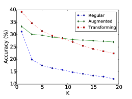
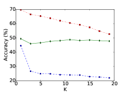
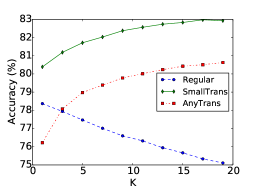
Fig. 4 shows KNN accuracy with respect to different $K$ values. For TFD, we can see that both regular KNN and transforming KNN degrade as $K$ increases. This is mainly due to the lack of examples in its KNN database: if $K$ is large, number of noise examples will be larger than true examples even the true examples might have higher similarities, which is also aggravated by the identity-imbalanced nature of TFD. In comparison, augmented KNN is the most robust to larger settings of $K$, due to the richness of same-identity examples in the KNN database.

For NORB, regular KNN accuracy decreases with increasing $K$. This is because without transforming distance, a test image should only be close to examples with the same class label and, with equal importance, the orientation in the KNN database. Therefore, test images cannot utilize many examples to provide effective distances. On the contrary, transforming KNN can utilize training examples regardless of their orientation, which results in an increasing robustness with increasing $K$.

(a) TFDs1 with feature distance

(b) TFDs2 with feature distance

(c) NORB with pixel distance

Figure 4: KNN accuracy vs. $K$. In (a) and (b), the dual-sided transforming KNN was performed and (b) shares the legend with (a). In (c), both SmallTrans and AnyTrans are single-sided.

4.4.3 KNN with a reduced database

(a) TFDs1 with feature distance

(b) TFDs2 with feature distance

(c) NORB with pixel distance

Figure 5: KNN accuracy with reduced databases. In (a) and (b), dual-sided transforming KNN was performed. In (c), both SmallTrans and AnyTrans are single-sided. $K=1$ for all plots.

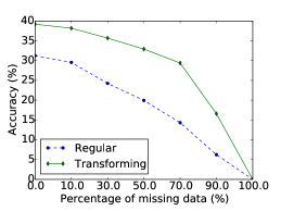
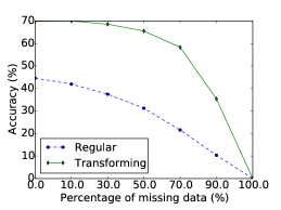
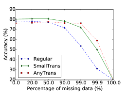
As previously mentioned, under transforming KNN, each example in the database can span a manifold and covers a “volume”. We examine this assumption by performing KNN on reduced databases and showing the relationship between accuracy and missing data rate (randomly discarded) in Fig. 5. For both TFD and NORB, transforming KNN works reasonably well with missing data. Their performance are still comparable to the regular KNN with complete database, when 70% (TFDs1), 80% (TFDs2) and even 99% (NORB, AnyTrans) data are missing.

For TFD, missing data results in missing identities. Therefore, no matter how good the relational model is, a performance drop is inevitable. In comparison, NORB contains only 5 classes. This makes it possible to maintain performance under a very high missing data rate. In Fig. 5 (c), AnyTrans KNN maintains its accuracy even when 99% data are missing (199 examples left in database); SmallTrans KNN is still better than regular KNN when 90% data are missing.

SmallTrans KNN performs better than AnyTrans KNN when the missing data rate is low, but degrades as the missing data rate increases. We suspect that the fgRBM has difficulty encoding complicated transformations (e.g. arbitrary 3D changes of objects). This conjecture (on the complexity of transformation) is supported by the fact that the best cross-validated fgRBM dimensionality is 128 for SmallTrans and 256 for AnyTrans.

Although the AnyTrans fgRBM might have learned less realistic transformations, it seems to be able to bridge large transformation gaps when the database is sparse. It maintains its performance even when 99% data are missing, and still provides a 60% accuracy when 99.9% data are missing. This hints at the potential of transforming KNN on “weakly” labeled datasets, where only a small portion of data have class labels and the majority of the data has weaker “relational labels” indicating image pairs. Relational labels can be acquired from video. Finally, using a reduced KNN database could potentially speed up transforming KNN by 100 times at test time. This alleviates the additional computational burden brought by test-time optimization.

5 Conclusion

The key novelty in our work is the idea of augmenting learned similarity functions with latent variables capturing factors of variation. Although we were inspired by the evidence of a mental faculty for the simulation of spatial transformations, we believe that this is just one example out of a richer class of dynamic similarity models achievable within this framework. That is to say, the proposed framework is generic, since it is composed of interchangeable components.

Nevertheless, performing inference or optimization over latent variables while comparing examples is much more computationally demanding than the typical “test-time” application of learned similarity models. This can be partially alleviated by a reduced need for large databases. Unfortunately our method precludes the use of approximate nearest neighbour techniques, which are typically used on large-scale problems of the type we considered. We have, however, achieved modest gains by parallelizing on GPUs. We believe that the computational cost is the main concern in considering similarity models with latent variables and we intend to address this issue in future work.

In each of the two datasets we considered, only a single transformation class was learned. Relational models like the fgRBM and relational autoencoder can, in theory, capture a rich set of transformations. Therefore another avenue of future work is demonstrating the efficacy of transforming similarity across a wider range of transformations.

References

- [1] Y. Bengio, F. Bastien, A. Bergeron, N. Boulanger-Lewandowski, T. Breuel, Y. Chherawala, M. Cisse, M. Côté, D. Erhan, J. Eustache, et al. Deep learners benefit more from out-of-distribution examples. In AISTATS, pages 164–172, 2011.
- [2] Y. Bengio, A. Courville, and P. Vincent. Representation learning: A review and new perspectives. Pattern Analysis and Machine Intelligence, IEEE Transactions on, 35(8):1798–1828, Aug 2013.
- [3] D. Cireşan, U. Meier, J. Masci, L. Gambardella, and J. Schmidhuber. Flexible, high performance convolutional neural networks for image classification. In IJCAI, 2011.
- [4] G. Dahl, M. Ranzato, A. Mohamed, and G. E Hinton. Phone recognition with the mean-covariance restricted boltzmann machine. In NIPS, pages 469–477, 2010.
- [5] J. Davis, B. Kulis, P. Jain, S. Sra, and I. Dhillon. Information-theoretic metric learning. In ICML, 2007.
- [6] Guillaume Desjardins, Aaron Courville, and Yoshua Bengio. Disentangling factors of variation via generative entangling. arXiv preprint arXiv:1210.5474, 2012.
- [7] Pedro F Felzenszwalb, Ross B Girshick, David McAllester, and Deva Ramanan. Object detection with discriminatively trained part-based models. Pattern Analysis and Machine Intelligence, IEEE Transactions on, 32(9):1627–1645, 2010.
- [8] P. Földiák. Learning invariance from transformation sequences. Neural Comput., 3(2):194–200, 1991.
- [9] J. Goldberger, S. Roweis, G. Hinton, and R. Salakhutdinov. Neighbourhood components analysis. In NIPS, 2004.
- [10] Michael U Gutmann, Valero Laparra, Aapo Hyvärinen, and Jesús Malo. Spatio-chromatic adaptation via higher-order canonical correlation analysis of natural images. PloS one, 9(2):e86481, 2014.
- [11] R. Hadsell, S. Chopra, and Y. LeCun. Dimensionality reduction by learning an invariant mapping. In CVPR, pages 1735–1742, 2006.
- [12] G. Hinton. Training products of experts by minimizing contrastive divergence. Neural Comput., 14(8):1771–1800, 2002.
- [13] G. Hinton and R. Salakhutdinov. Reducing the dimensionality of data with neural networks. Science, 313(5786):504–507, 2006.
- [14] Harold Hotelling. Relations between two sets of variates. Biometrika, pages 321–377, 1936.
- [15] H. Kamyshanska and R. Memisevic. On autoencoder scoring. In ICML, pages 720–728, 2013.
- [16] Y. Karklin and M. Lewicki. Emergence of complex cell properties by learning to generalize in natural scenes. Nature, 457(7225):83–86, 2009.
- [17] K. Konda, R. Memisevic, and V. Michalski. The role of spatio-temporal synchrony in the encoding of motion. In Proc. of International Conference on Learning Representations, 2014.
- [18] Y. LeCun, L. Bottou, Y. Bengio, and P. Haffner. Gradient-based learning applied to document recognition. Proc. IEEE, 86(11):2278–2324, 1998.
- [19] Y. LeCun, Fu J. Huang, and L. Bottou. Learning methods for generic object recognition with invariance to pose and lighting. In CVPR, volume 2, pages II–97. IEEE, 2004.
- [20] Q. Liao, J. Leibo, and T. Poggio. Learning invariant representations and applications to face verification. In NIPS, pages 3057–3065, 2013.
- [21] Thomas Melzer, Michael Reiter, and Horst Bischof. Appearance models based on kernel canonical correlation analysis. Pattern recognition, 36(9):1961–1971, 2003.
- [22] R. Memisevic. Gradient-based learning of higher-order image features. In ICCV. IEEE, 2011.
- [23] R. Memisevic. Learning to relate images. IEEE TPAMI, 35(8):1829–1846, 2013.
- [24] R. Memisevic and G. Hinton. Unsupervised learning of image transformations. In CVPR, 2007.
- [25] R. Memisevic and G. Hinton. Learning to represent spatial transformations with factored higher-order boltzmann machines. Neural Comput., 22(6):1473–1492, 2010.
- [26] H. Mobahi, R. Collobert, and J. Weston. Deep learning from temporal coherence in video. In ICML, 2009.
- [27] M. Paulin, J. Revaud, Z. Harchaoui, F. Perronnin, and C. Schmid. Transformation Pursuit for Image Classification. In CVPR, Columbus, États-Unis, April 2014.
- [28] N. Pinto, D. Cox, and J. DiCarlo. Why is real-world visual object recognition hard? PLoS compbiol, 4(1):e27, 2008.
- [29] M. Ranzato and G. Hinton. Modeling pixel means and covariances using factorized third-order boltzmann machines. In CVPR, pages 2551–2558. IEEE, 2010.
- [30] Scott Reed, Kihyuk Sohn, Yuting Zhang, and Honglak Lee. Learning to disentangle factors of variation with manifold interaction.
- [31] S. Rifai, P. Vincent, X. Muller, X. Glorot, and Y. Bengio. Contractive auto-encoders: Explicit invariance during feature extraction. In ICML, pages 833–840, 2011.
- [32] R. Shepard, J. Metzler, et al. Mental rotation of three-dimensional objects. Science, 171(3972):701, 1971.
- [33] K. Sohn and H. Lee. Learning invariant representations with local transformations. In ICML, 2012.
- [34] Rachel Sparks and Anant Madabhushi. Novel morphometric based classification via diffeomorphic based shape representation using manifold learning. In Medical Image Computing and Computer-Assisted Intervention–MICCAI 2010, pages 658–665. Springer, 2010.
- [35] J. Susskind, A. Anderson, and G. Hinton. The toronto face database. U of Toronto, Tech. Rep, 2010.
- [36] J. Susskind, R. Memisevic, G. Hinton, and M. Pollefeys. Modeling the joint density of two images under a variety of transformations. In CVPR, pages 2793–2800. IEEE, 2011.
- [37] G. Taylor, R. Fergus, Y. LeCun, and C. Bregler. Convolutional learning of spatio-temporal features. In ECCV, pages 140–153. Springer, 2010.