Impact of polarisation on the intrinsic CMB bispectrum

Abstract

We compute the bispectrum induced in the cosmic microwave background (CMB) temperature and polarisation by the evolution of the primordial density perturbations using the second-order Boltzmann code SONG. We show that adding polarisation increases the signal-to-noise ratio by a factor four with respect to temperature alone and we estimate the observability of this intrinsic bispectrum and the bias it induces on measurements of primordial non-Gaussianity. When including all physical effects except the late-time non-linear evolution, we find for the intrinsic bispectrum a signal-to-noise of $S/N=3.8,\,2.9,\,1.6$ and $0.5$ for, respectively, an ideal experiment with an angular resolution of ${\ell_{\text{max}}}=3000$, the proposed CMB surveys PRISM and COrE, and Planck’s polarised data; the bulk of this signal comes from the $E$-polarisation and from squeezed configurations. We discuss how CMB lensing is expected to reduce these estimates as it suppresses the bispectrum for squeezed configurations and contributes to the noise in the estimator. We find that the presence of the intrinsic bispectrum will bias a measurement of primordial non-Gaussianity of local type by $f_{\text{NL}}^{\text{intr}}=0.66$ for an ideal experiment with ${\ell_{\text{max}}}=3000$. Finally, we verify the robustness of our results by reproducing the analytical approximation for the squeezed-limit bispectrum in the general polarised case.

Introduction

The three-point function, or bispectrum, of the cosmic microwave background (CMB) is directly linked to non-Gaussian features in the primordial fluctuations from which the CMB evolved Komatsu and Spergel (2001); Komatsu (2010); Liguori et al. (2010); Yadav and Wandelt (2010); Bartolo et al. (2010). Measuring the CMB bispectrum is therefore equivalent to opening a window to the early Universe. In particular the temperature maps measured by the Planck CMB survey Planck Collaboration (2013a) provide the most stringent constraint on the amplitude $f_{\text{NL}}$ of primordial non-Gaussianity of the local type Komatsu and Spergel (2001); Gangui et al. (1994); Verde et al. (2000): $f_{\text{NL}}=2.7\,\pm\,5.8\;$. Furthermore, the polarised maps, expected from Planck by the end of 2014, will be used to refine the $f_{\text{NL}}$ measurement and reduce the error by approximately a factor two Babich et al. (2004); Komatsu et al. (2005); Yadav et al. (2007, 2008); Yadav and Wandelt (2010).

However not all of the observed non-Gaussianity is of primordial origin. Indeed, a bispectrum arises in the CMB even for Gaussian initial conditions in the primordial curvature perturbation Lyth and Rodríguez (2005) due to non-linear dynamics such as CMB photons scattering off free electrons and their propagation along a perturbed geodesic in an inhomogeneous Universe. This intrinsic bispectrum is an interesting signal in its own right as it contains information on such processes. Furthermore, if not correctly estimated and subtracted from the CMB maps, it will provide a bias in the estimate of primordial $f_{\text{NL}}$.

Computing the intrinsic bispectrum requires solving the Einstein and Boltzmann equations up to second order in the cosmological perturbations. These have been studied in great detail Pitrou (2009); Pitrou et al. (2010a); Beneke and Fidler (2010); Naruko et al. (2013); Bartolo et al. (2006, 2007) and approximate solutions have been found in specific limits Bartolo et al. (2004a, b); Boubekeur et al. (2009); Senatore et al. (2009a, b); Nitta et al. (2009). In particular, the intrinsic bispectrum can be obtained analytically in the so-called “squeezed” limit, where one of the three scales is much larger than the others Creminelli and Zaldarriaga (2004); Creminelli et al. (2011); Bartolo et al. (2012); Lewis (2012). However, for arbitrary configurations, the intrinsic bispectrum has to be computed numerically. Numerical convergence is now being reached as the latest numerical codes Huang and Vernizzi (2013); Su et al. (2012); Pettinari et al. (2013); Huang and Vernizzi (2013) obtain consistent results. When considering only the temperature bispectrum, these codes find the bias induced on $f_{\text{NL}}$ by second-order effects to be of order unity, and the intrinsic bispectrum to be unobservable by Planck, its signal-to-noise ratio reaching unity only for an ideal experiment with an angular resolution of ${\ell_{\text{max}}}=3000$.

In this letter, we extend the studies discussed above by including for the first time CMB polarisation, and show that the intrinsic bispectrum signal is enhanced considerably compared to the primordial signals, making it potentially observable in the next generation CMB missions, such as COrE The COrE Collaboration (2011) and PRISM PRISM Collaboration (2013). We also explore the impact that gravitational lensing has on the observability of the intrinsic bispectrum, both by reducing the amplitude of the intrinsic signal and by providing an additional source of noise in the measurement of the bispectra.

Method

We recently studied the intrinsic temperature bispectrum Pettinari et al. (2013); Pettinari (2014) and the $B$-mode polarisation induced from non-linear dynamics Fidler et al. (2014). Using the tools developed in the latter paper we extend our bispectrum analysis to include polarisation. Throughout, we assume the primordial non-Gaussianity to be negligible ($f_{\text{NL}}=0$).

We employ the system of coupled Boltzmann-Einstein equations at second order describing the non-linear evolution of the different species Bartolo et al. (2006, 2007); Pitrou (2009); Beneke and Fidler (2010); Naruko et al. (2013) and work in the Poisson gauge Bertschinger (1996). The Boltzmann equation consists of a Liouville term, accounting for particle propagation in an inhomogeneous space-time, and a collision term describing particle interactions, i.e. Compton scattering for CMB photons. We characterise photons by their brightness moments $\Delta_{n}$ with the composite index $n$ including the angular harmonic indices $\ell m$ and the polarisation index $X=T,E,B$. The photon intensity is characterised by $X=T$, while $E$ and $B$ characterise the CMB polarisation. The Boltzmann equation for $\Delta_{n}$ reads

$$\dot{\Delta}_{n}\;+\;k\,\Sigma_{nn^{\prime}}\Delta_{n^{\prime}}\;+\;\mathcal{M}_{n}\;+\;\mathcal{Q}^{L}_{n}\;=\;\mathfrak{C}_{n}\;,$$ (1)

where $k$ is the Fourier wavevector of the perturbation, and the free-streaming matrix $\Sigma_{nn^{\prime}}$ encodes the excitation of high-$\ell$ moments over time. We have denoted the terms containing only metric perturbations by $\,\mathcal{M}_{n}$, while $\,\mathcal{Q}^{L}_{n}\,$ describes the effect of the metric on the photon perturbations, that is the redshift, time-delay and lensing effects. The collision term

$$\mathfrak{C}_{n}\;=\;-|\dot{\kappa}|\,\left(\;\Delta_{n}\;-\;\Gamma_{nn^{\prime}}\Delta_{n^{\prime}}\;-\;\mathcal{Q}^{C}_{n}\,\,\right)\;,$$ (2)

is proportional to the Compton scattering rate $|\dot{\kappa}|$ and consists of the purely second-order gain and loss terms, and quadratic contributions $\,|\dot{\kappa}|\,\mathcal{Q}^{C}_{n}$. The explicit form and detailed description of all terms can be found in Ref. Fidler et al. (2014); Pettinari et al. (2013); Beneke and Fidler (2010).

After recombination photons stream freely, so that at conformal time $\eta$ the higher multipoles with $\ell\approx k\,(\eta-\eta_{\text{rec}})$ are excited, making the numerical computation of the photon moments up to today ($\eta_{0}$) impractical using the full Boltzmann-Einstein equations. In SONG we instead compute the photon perturbations after recombination using the line-of-sight integration Seljak and Zaldarriaga (1996):

$$\Delta_{n}(\eta_{0})\;=\;\int_{0}^{\eta_{0}}d\eta\,e^{-\kappa(\eta)}\;j_{nn^{\prime}}(k(\eta_{0}-\eta))\;\mathcal{S}_{n^{\prime}}(\eta)\;,$$ (3)

with the streaming functions $j_{nn^{\prime}}$ specified in Ref. Pettinari (2014); Beneke et al. (2011), and the line-of-sight source function $\mathcal{S}_{n}$ given by

$$\mathcal{S}_{n}\;=\;-\mathcal{M}_{n}\,-\,\mathcal{Q}^{L}_{n}\,+\,|\dot{\kappa}|\left(\Gamma_{nn^{\prime}}\Delta_{n^{\prime}}+\mathcal{Q}^{C}_{n}\right)\;.$$ (4)

We first solve the full second-order Boltzmann-Einstein hierarchy to build $\mathcal{S}_{n}$ until the time of recombination, as described in Ref. Pettinari et al. (2013); Fidler et al. (2014); Pettinari (2014), and then compute the line-of-sight integral in Eq. 3 to obtain the photon perturbations today.

Recently Huang & Vernizzi (2013) Huang and Vernizzi (2013) clarified the relation between the remapping and second-order Boltzmann approaches to lensing, while Su & Lim (2014) Su and Lim (2014) developed an alternative non-perturbative treatment of lensing involving a Dyson series. These works allow us to identify the lensing and time-delay terms in the second-order equations and remove them from the line-of-sight sources, because, at second order, their effect along the line-of-sight results in the well-known CMB-lensing bispectrum Lewis et al. (2011) plus a small residual Huang and Vernizzi (2013). We do include the redshift term by using the $\widetilde{\Delta}$ transformation of variables first introduced in Ref. Huang and Vernizzi (2013) and later generalised to the polarised case in Ref. Fidler et al. (2014):

$$\begin{aligned} \widetilde{\Delta}_{T,\ell m}\;=&\;\Delta_{T,\ell m}-\frac{1}{2}\,i^{L}\left(\begin{array}[]{cc|c}\ell^{\prime}&\ell^{\prime\prime}&\ell\\ m^{\prime}&m^{\prime\prime}&m\end{array}\right)\left(\begin{array}[]{cc|c}\ell^{\prime}&\ell^{\prime\prime}&\ell\\ 0&0&0\end{array}\right)\\[7.11317pt] &\times\Delta_{T,\ell^{\prime}m^{\prime}}\Delta_{T,\ell^{\prime\prime}m^{\prime\prime}}\;,\end{aligned}$$ (5)

$$\begin{aligned} \widetilde{\Delta}_{E,\ell m}\;=&\;\Delta_{E,\ell m}-i^{L}\left(\begin{array}[]{cc|c}\ell^{\prime}&\ell^{\prime\prime}&\ell\\ m^{\prime}&m^{\prime\prime}&m\end{array}\right)\left(\begin{array}[]{cc|c}\ell^{\prime}&\ell^{\prime\prime}&\ell\\ 0&2&2\end{array}\right)\\[7.11317pt] &\times\Delta_{T,\ell^{\prime}m^{\prime}}\Delta_{E,\ell^{\prime\prime}m^{\prime\prime}}\;,\end{aligned}$$

for even $L=\ell-\ell^{\prime}-\ell^{\prime\prime}$. A summation over $\ell^{\prime},\ell^{\prime\prime},m^{\prime},m^{\prime\prime}$ is implied and the parentheses symbols represent the Clebsch-Gordan coefficients.

After using the line-of-sight integration to obtain $\Delta_{n}(\eta_{0})$, we relate it to the bolometric temperature perturbation $a^{X}_{\ell m}$ Fidler et al. (2014); Pitrou and Stebbins (2014); Pitrou et al. (2010b), and compute its full-sky bispectrum:

$$B^{XYZ}_{{\ell_{1}}{\ell_{2}}{\ell_{3}}} =\sum\limits_{m_{1}m_{2}m_{3}}\;\begin{pmatrix}{{\ell_{1}}\!}&{{\ell_{2}}\!}&{{\ell_{3}}}\\ {m_{1}\!}&{m_{2}\!}&{m_{3}}\end{pmatrix}\;\left\langle a^{X}_{{{\ell_{1}}m_{1}}}\,a^{Y}_{{{\ell_{2}}m_{2}}}\,a^{Z}_{{{\ell_{3}}m_{3}}}\right\rangle$$

$$=\;\begin{pmatrix}{{\ell_{1}}\!}&{{\ell_{2}}\!}&{{\ell_{3}}}\\ {0\!}&{0\!}&{0}\end{pmatrix}\;b^{XYZ}_{{\ell_{1}}{\ell_{2}}{\ell_{3}}}\;,$$ (6)

where $X,Y,Z$ are either $T$ or $E$. This computation is done in the same way as in our previous work Pettinari et al. (2013), where we focussed on the unpolarised scalar contributions to the bispectrum, corresponding to the $m=0$ sources in Eq. 4. In this letter, we also include $m\neq 0$ contributions up to $|m|=3$ following Ref. Pettinari (2014) and find that they are subdominant with respect to the $m=0$ modes as they consist of about $3\%$ of the total signal.

In the calculations below, we have assumed the Planck best-fit $\Lambda$CDM cosmology Planck Collaboration (2013b) where $h=0.678$, $\Omega_{b}=0.0483$, $\Omega_{\text{cdm}}=0.259$, $\Omega_{\Lambda}=0.693$, $A_{s}={2.214}\times 10^{-9}$, $n_{s}=0.961$, $N_{\text{eff}}=3.04$, $\kappa_{\text{reio}}=0.095$. We also assume adiabatic initial conditions with a vanishing primordial tensor-to-scalar ratio ($r=0$).

Polarisation impact

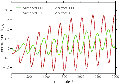
Figure 1: Numerical intrinsic bispectrum produced by SONG, together with the squeezed-limit approximation in Eq. 7, with ${\ell_{1}}=6$ and ${\ell_{2}}={\ell_{3}}=\ell$, for $TTT$ and $EEE$. We normalise the curves with respect to the squeezed limit for the local-type bispectrum Gangui et al. (1994); Komatsu and Spergel (2001) with $f_{\text{NL}}=5$, that is $6\,C_{{\ell_{1}}}^{X\zeta}\left(\,C^{YZ}_{{\ell_{2}}}\,+\,C^{YZ}_{{\ell_{3}}}\,\right)\,$.

For squeezed configurations (${\ell_{1}}\ll{\ell_{2}},\,{\ell_{3}}$), where the long-wavelength mode is within the horizon today but was not at recombination (${\ell_{1}}\ll 200$), the intrinsic bispectrum is known analytically. In this case, the super-horizon curvature perturbation at recombination, $\zeta$, acts as a perturbation to the background curvature that dilates the observed angular scale of the small-scale CMB anisotropies. Large and small scales are thus correlated and a squeezed intrinsic bispectrum arises that is proportional to the correlation between the large-scale CMB anisotropies and $\zeta$. In multipole space, a dilation corresponds to a sideways shift in $\ell$, so that the more sharply peaked the small-scale power spectrum, the bigger the change in power. As a result, the intrinsic bispectrum in the squeezed limit is proportional to the derivative of the small-scale power spectrum Creminelli and Zaldarriaga (2004); Creminelli et al. (2011); Bartolo et al. (2012); Lewis (2012):

$$b^{\text{sq},XYZ}_{{\ell_{1}}{\ell_{2}}{\ell_{3}}}\;=\; -\frac{1}{2}\;C_{{\ell_{1}}}^{X\zeta}\;\left[\,\frac{\textrm{d}\,({\ell_{2}}^{2}\,C^{YZ}_{{\ell_{2}}})}{{\ell_{2}}\,\textrm{d}\,{\ell_{2}}}\,+\,\frac{\textrm{d}\,({\ell_{3}}^{2}\,C^{YZ}_{{\ell_{3}}})}{{\ell_{3}}\,\textrm{d}\,{\ell_{3}}}\,\right]$$ (7)

$$+C^{XT}_{{\ell_{1}}}\;\left[\,\delta_{ZT}\,C^{YT}_{{\ell_{2}}}\,+\,\delta_{YT}\,C^{ZT}_{{\ell_{3}}}\,\right]\;,$$

where $X,Y,Z$ are either $T$ or $E$ and the angular power spectra are defined by $\left\langle\,{a^{X}_{\ell m}\,a^{Y*}_{\ell^{\prime}m^{\prime}}}\,\right\rangle\;\equiv\;C^{XY}_{\ell}\,\delta_{\ell\ell^{\prime}}\,\delta_{mm^{\prime}}\;.$ The second line in Eq. 7 represents the subdominant effect known as redshift modulation Lewis (2012). In Figure 1, we show that SONG’s numerical bispectra match the analytical approximation in the squeezed limit at percent-level precision.

In SONG we truncate the line-of-sight integration in Eq. 3 at recombination and thus neglect the second-order scattering sources at reionisation. Their computation is challenging as it involves summations over high-$\ell$ multipoles at late times. In any case, a second-order treatment would still be insufficient, as non-linear effects are relevant at the time of reionisation. We do however include reionisation at the background and linear level. The squeezed formula of Eq. 7 works at the same level since $\zeta$ is defined to be the value of the curvature perturbation at recombination, which is the source of the small-scale perturbations being modulated; hence the match with SONG for squeezed shapes shown in Figure 1.

The linear temperature anisotropies observed today are sourced by density and velocity perturbations at recombination. Since these are out-of-phase in $\ell$ space, the resulting acoustic peaks are blurred. On the other hand, the peaks of the $E$ polarisation spectrum are sharper as their only source is the quadrupole induced by Compton scattering. It follows that the logarithmic derivatives in Eq. 7 normalised to $C^{YZ}_{\ell}$ will be larger for polarisation than for temperature. This enhancement is about a factor $2.5$ in magnitude across the whole $\ell$-range (Figure 1) and leads to a larger signal-to-noise ratio for the polarised bispectra. Note, however, that the temperature bispectrum, $TTT$, is still much larger than the polarisation one, $EEE$, as $C_{{\ell_{1}}}^{T\zeta}\approx 100\,C_{{\ell_{1}}}^{E\zeta}$ for ${\ell_{1}}<200$ Lewis (2012).

In order to quantify the observability of the intrinsic bispectrum and its bias on a primordial measurement of $f_{\text{NL}}$, we build the Fisher matrix element in the general polarised case as Babich et al. (2004); Yadav et al. (2008); Komatsu and Spergel (2001); Lewis et al. (2011)

$$F^{(i),(j)}\;=\;\sum\limits_{ABC,XYZ}\;\sum\limits_{2\leq{\ell_{1}}\leq{\ell_{2}}\leq{\ell_{3}}}^{{\ell_{\text{max}}}}\frac{1}{\Delta_{{\ell_{1}}{\ell_{2}}{\ell_{3}}}}\;$$ (8)

$$\;\times\;B^{(i),ABC}_{{\ell_{1}}{\ell_{2}}{\ell_{3}}}\;\left(\widetilde{C}_{\text{tot}}^{-1}\right)^{AX}_{\ell_{1}}\;\left(\widetilde{C}_{\text{tot}}^{-1}\right)^{BY}_{\ell_{2}}\;\left(\widetilde{C}_{\text{tot}}^{-1}\right)^{CZ}_{\ell_{3}}\;B^{(j),XYZ}_{{\ell_{1}}{\ell_{2}}{\ell_{3}}}\;,$$

where $\,\Delta_{{\ell_{1}}{\ell_{2}}{\ell_{3}}}=1,2,6\,$ for triangles with no, two or three equal sides, $\,{\ell_{\text{max}}}$ is limited by the finite angular resolution of the survey and $\,\widetilde{C}_{\text{tot}}^{XY}$ is given by the sum of the lensed spectrum and a noise term to account for the sensitivity of the survey Pogosian et al. (2005); Knox (1995). The first sum involves all possible pairs of the eight bispectra ($TTT$, $TTE$, $TET$, $ETT$, $EET$, $ETE$, $TEE$, $EEE$), while the product of three $\widetilde{C}^{-1}_{\text{tot}}$ represents their covariance. The observability of the intrinsic bispectrum is quantified by its signal-to-noise ratio $S/N=\sqrt{F^{\text{intr},\text{intr}}}\,$, while the bias it induces on a measurement of local-type $f_{\text{NL}}$ is $\,f_{\text{NL}}^{\text{intr}}=F^{\text{loc},\text{intr}}/F^{\text{loc},\text{loc}}\,$.

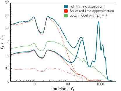
Figure 2: Contributions (per $\ln{\ell_{1}}$) to the inverse variance, $\,F^{\,({i}),({i})}\,$, of the intrinsic bispectrum as a function of the smallest multipole in the sum, ${\ell_{1}}$, considering an ideal experiment with ${\ell_{\text{max}}}=3000$. In this plot, the area below each bispectrum curve is proportional to the square of its signal-to-noise ratio. The full bispectrum computed with SONG (thick-blue lines) exhibits distinctive peaks on subhorizon scales (${\ell_{1}}>100$), while on larger scales it tracks the the squeezed-limit approximation (thin red lines). The dashed lines do not include lensing variance, which reduces the signal-to-noise only on superhorizon scales; the lensed bispectrum in the squeezed limit is shown by the dotted line. For reference, we also include the curve expected from a local-type bispectrum with $f_{\text{NL}}=4$ (green solid line).

In Figure 2 we show the signal-to-noise as a function of ${\ell_{1}}$, the smallest multipole in the Fisher matrix sum, for an ideal CMB survey with a resolution of ${\ell_{\text{max}}}=3000$. On superhorizon scales (${\ell_{1}}\ll 200$), the intrinsic bispectrum computed by SONG agrees well with the squeezed-limit formula, as expected. The subhorizon effects computed by SONG become important for ${\ell_{1}}>100$ and give rise to several acoustic peaks. The signal associated to the subhorizon peaks is given by the square root of the area below the curve, and amounts to $S/N=1.6$ and $2.7$ for ${\ell_{\text{max}}}=3000$ and $4000$, respectively; most of this signal comes from squeezed triangles. Note that these effects cannot be treated in the analytical approximation in Eq. 7 and hence need to be computed using a full second-order code like SONG. Furthermore, we find that the relative importance of the subhorizon effects increases with ${\ell_{\text{max}}}$.

Lensing effects

The Fisher matrix estimator of Eq. 8 is optimal only under the assumption of a nearly Gaussian CMB. However, the gravitational lensing of CMB photons generates a non-Gaussian signal that must be accounted for in the covariance matrix; not doing so would overestimate the significance for a detection of the intrinsic bispectrum Lewis et al. (2011); Hanson et al. (2009). We account for this lensing variance in the estimator following the analytic approach of Ref. Lewis et al. (2011), which is valid for squeezed configurations.

We find that lensing variance degrades the intrinsic signal from ${\ell_{1}}<200$ by approximately a factor $\sqrt{2}$, while leaving the signal from smaller scales unaltered, as can be seen by comparing the dashed and solid curves in Figure 2. The reason is that most of the signal below ${\ell_{1}}<200$ comes the squeezed configurations described by the analytical formula in Eq. 7, which are highly degenerate with the isotropic part of lensing (i.e., convergence) Creminelli and Zaldarriaga (2004); Creminelli et al. (2011); Lewis (2012). As a result, the added noise from lensing convergence significantly reduces our ability to detect the intrinsic bispectrum for ${\ell_{1}}<200$. On the other hand, we find that the intrinsic signal does not correlate significantly with convergence or shear modes on smaller scales and is thus not affected by lensing variance. After correcting for lensing variance, the subhorizon effects constitute about $40\%$ and $50\%$ of the intrinsic signal squared for ${\ell_{\text{max}}}=3000$ and $4000$, respectively, and a larger fraction for higher resolutions.

In addition to the lensing-induced variance, two other effects of gravitational lensing may affect the measurement of the intrinsic bispectrum. First, the correlation between the photon intensity and the lensing deflection angle results in the emergence of a CMB-lensing bispectrum Spergel and Goldberg (1999); Goldberg and Spergel (1999); Seljak and Zaldarriaga (1999) which was recently detected by the Planck experiment Planck Collaboration (2013a), and corresponds to the lensing terms we dropped in the line-of-sight integration. The isotropic part of the CMB-lensing bispectrum is known to be degenerate with the intrinsic bispectrum Creminelli and Zaldarriaga (2004); Creminelli et al. (2011); Lewis (2012) in the squeezed limit and might therefore contaminate a measurement of the latter. To quantify this effect we include the amplitude of the CMB-lensing bispectrum in our Fisher matrix and marginalise over it. We find that, in the full polarised case and including lensing variance, the intrinsic and lensing bispectra have a correlation of $0.6\%$ and, therefore, the intrinsic $S/N$ is degraded only by about $0.002\%$. These numbers suggest that the CMB-lensing bispectrum is different enough from the intrinsic bispectrum to allow a clear separation of the effects, in analogy to the case of the local $f_{\text{NL}}$ template Lewis et al. (2011); Planck Collaboration (2013a). Note that this separation cannot be used to reduce the impact of lensing variance, as the signal cannot be used to reduce the noise in the estimator.

Secondly, CMB lensing distorts the observed shape of the intrinsic bispectrum in a non-perturbative way. In the squeezed limit, the lensed bispectrum is obtained by substituting the power spectrum $C_{\ell}^{YZ}$ in Eq. 7 with its lensed counterpart, $\widetilde{C}_{\ell}^{YZ}$ Lewis (2012); Lewis et al. (2011). This results in a smaller bispectrum as the derivatives in Eq. 7 now act on a smoother function. The $S/N$ from squeezed configurations is consequently reduced by a factor of approximately $\,\sqrt{2}\,$ for ${\ell_{\text{max}}}=3000$, as can be seen by comparing the solid and dotted red curves in Figure 2. However, this suppression is only valid in the squeezed case; for arbitrary configurations one has to resort to a more general approach Cooray et al. (2008); Hanson et al. (2009); Pearson et al. (2012), which we will address in future work. Here we focus on the unlensed intrinsic bispectra.

Observational implications

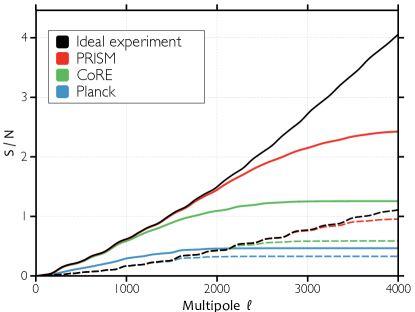
Figure 3: Signal-to-noise ratio of the intrinsic bispectrum for the four experiments described in the text as a function of the maximum resolution $\ell_{\text{max}}$, including lensing variance and excluding the lensing of the bispectrum. The solid curves include all eight temperature and polarisation bispectra, the dashed ones only temperature.

In Figure 3 we present the signal-to-noise ratio of the intrinsic bispectrum for four experiments as a function of the maximum resolution $\ell_{\text{max}}$. We consider an ideal experiment, the proposed CMB surveys PRISM PRISM Collaboration (2013) and COrE The COrE Collaboration (2011), and Planck polarisation data. We only employ frequencies between $100$ and $300$ GHz, where the CMB signal peaks, and assume full-sky observations. Through numerical convergence tests for the key numerical parameters, we have ensured these results are stable at the percent-level.

Figure 3 shows that the angular resolution of the CMB survey strongly affects the detectability of the intrinsic bispectrum. With a resolution of ${\ell_{\text{max}}}=3000$, an ideal experiment would observe the intrinsic bispectrum at the $2.7\sigma$ level, while PRISM, COrE and Planck polarised data would yield $2.1\sigma,1.3\sigma,0.46\sigma$, respectively. When we account for the lensing of the bispectrum in the squeezed regime via the analytical formula in Eq. 7, these numbers reduce to $2.1\sigma,1.8\sigma,1.1\sigma,0.41\sigma$.

Another important feature of Figure 3 is that most of the signal in the intrinsic bispectrum comes from $E$-polarisation rather than temperature, despite the fact that only a $10\%$ fraction of the CMB anisotropies are polarised. The reason is twofold. First, the dilation effect that generates the intrinsic bispectrum on squeezed scales is $\sim\!2.5$ times more efficient for polarisation than for temperature, as shown in Figure 1. Secondly, as long as the instrumental noise is low enough, both temperature and polarisation are sample-variance limited, so that the polarisation bispectrum variance is also suppressed compared to that of the temperature. In principle, the same argument applies to $B$-polarisation. The intrinsic $B$-signal, however, is sourced by non-scalar sources that are geometrically suppressed Fidler et al. (2014) making it smaller than the $E$-signal and thus likely to be dominated by lensing Zaldarriaga and Seljak (1998); Lewis and Challinor (2006) and instrumental noise.

We find the bias to the local-type $f_{\text{NL}}$ for an ideal experiment with resolution $\,{\ell_{\text{max}}}=3000\,$ to be $\,f_{\text{NL}}^{\text{intr}}=1.33,1.50,1.51\,$ for temperature, polarisation and the two probes combined, respectively. Including lensing variance reduces the bias to $f_{\text{NL}}^{\text{intr}}=0.95,0.61,0.66$. This suppression is due to the intrinsic bispectrum being affected by lensing variance more than the local template. The bias is further reduced by varying the experimental setup: for PRISM, CoRE and Planck polarised data we find $f_{\text{NL}}^{\text{intr}}=0.58,0.45,0.37$, respectively, considering lensing variance and both temperature and polarisation.

Conclusions

Including polarisation is crucial to extract all the information contained in the CMB. In this letter we have extended previous analyses of the intrinsic bispectrum Pettinari et al. (2013); Huang and Vernizzi (2013); Su et al. (2012) and shown that it is particularly sensitive to polarisation due to the sharp acoustic peaks in the $E$-mode power spectrum. Using a Fisher matrix approach, we showed that the eight combined bispectra generate a signal-to-noise ratio four times larger with respect to the temperature-only case, making the signal potentially observable at the $2\sigma$ level in future high-resolution missions, such as PRISM PRISM Collaboration (2013) or an improved version of COrE The COrE Collaboration (2011). Despite the enhancement of the intrinsic signal, we still find its contamination to the local-type primordial $f_{\text{NL}}$ to be comparable to the unpolarised case.

For squeezed configurations, the gravitational lensing of CMB photons limits the possibility of observing the intrinsic bispectrum by adding extra variance and by reducing its observed amplitude. These effects combine to reduce the signal-to-noise by a factor of two. However, on subhorizon scales, where full second-order codes such as SONG are crucial, the added variance does not limit the detectability.

Here we have included the effects of reionisation and the lensing of the bispectrum only in an approximate way, focussing on their impact in the squeezed limit. Reionisation could lead to additional intrinsic contributions in a full second-order treatment, while lensing could affect the signal on subhorizon scales. We will examine these questions in future work.

References

- Komatsu and Spergel (2001) E. Komatsu and D. N. Spergel, Phys. Rev. D 63, 063002 (2001), eprint astro-ph/0005036.
- Komatsu (2010) E. Komatsu, Classical and Quantum Gravity 27, 124010 (2010), eprint 1003.6097.
- Liguori et al. (2010) M. Liguori, E. Sefusatti, J. R. Fergusson, and E. P. S. Shellard, Advances in Astronomy (2010), eprint 1001.4707.
- Yadav and Wandelt (2010) A. P. S. Yadav and B. D. Wandelt, Advances in Astronomy (2010), eprint 1006.0275.
- Bartolo et al. (2010) N. Bartolo, S. Matarrese, and A. Riotto, Advances in Astronomy (2010), eprint 1001.3957.
- Planck Collaboration (2013a) Planck Collaboration, ArXiv e-prints (2013a), eprint 1303.5084.
- Gangui et al. (1994) A. Gangui, F. Lucchin, S. Matarrese, and S. Mollerach, ApJ 430, 447 (1994), eprint astro-ph/9312033.
- Verde et al. (2000) L. Verde, L. Wang, A. F. Heavens, and M. Kamionkowski, MNRAS 313, 141 (2000), eprint astro-ph/9906301.
- Babich et al. (2004) D. Babich, P. Creminelli, and M. Zaldarriaga, J. Cosmology Astropart. Phys 8, 9 (2004), eprint astro-ph/0405356.
- Komatsu et al. (2005) E. Komatsu, D. N. Spergel, and B. D. Wandelt, ApJ 634, 14 (2005), eprint astro-ph/0305189.
- Yadav et al. (2007) A. P. S. Yadav, E. Komatsu, and B. D. Wandelt, ApJ 664, 680 (2007), eprint astro-ph/0701921.
- Yadav et al. (2008) A. P. S. Yadav, E. Komatsu, B. D. Wandelt, M. Liguori, F. K. Hansen, and S. Matarrese, ApJ 678, 578 (2008), eprint 0711.4933.
- Lyth and Rodríguez (2005) D. H. Lyth and Y. Rodríguez, Physical Review Letters 95, 121302 (2005), eprint astro-ph/0504045.
- Pitrou (2009) C. Pitrou, Classical and Quantum Gravity 26, 065006 (2009), eprint 0809.3036.
- Pitrou et al. (2010a) C. Pitrou, J. Uzan, and F. Bernardeau, J. Cosmology Astropart. Phys 7, 3 (2010a), eprint 1003.0481.
- Beneke and Fidler (2010) M. Beneke and C. Fidler, Phys. Rev. D 82, 063509 (2010), eprint 1003.1834.
- Naruko et al. (2013) A. Naruko, C. Pitrou, K. Koyama, and M. Sasaki, ArXiv e-prints (2013), eprint 1304.6929.
- Bartolo et al. (2006) N. Bartolo, S. Matarrese, and A. Riotto, Journal of Cosmology and Astro-Particle Physics 6, 24 (2006), eprint astro-ph/0604416.
- Bartolo et al. (2007) N. Bartolo, S. Matarrese, and A. Riotto, Journal of Cosmology and Astro-Particle Physics 1, 19 (2007), eprint astro-ph/0610110.
- Bartolo et al. (2004a) N. Bartolo, S. Matarrese, and A. Riotto, J. Cosmology Astropart. Phys 1, 003 (2004a), eprint astro-ph/0309692.
- Bartolo et al. (2004b) N. Bartolo, S. Matarrese, and A. Riotto, Physical Review Letters 93, 231301 (2004b), eprint astro-ph/0407505.
- Boubekeur et al. (2009) L. Boubekeur, P. Creminelli, G. D’Amico, J. Noreña, and F. Vernizzi, J. Cosmology Astropart. Phys 8, 029 (2009), eprint 0906.0980.
- Senatore et al. (2009a) L. Senatore, S. Tassev, and M. Zaldarriaga, J. Cosmology Astropart. Phys 9, 38 (2009a), eprint 0812.3658.
- Senatore et al. (2009b) L. Senatore, S. Tassev, and M. Zaldarriaga, J. Cosmology Astropart. Phys 8, 031 (2009b), eprint 0812.3652.
- Nitta et al. (2009) D. Nitta, E. Komatsu, N. Bartolo, S. Matarrese, and A. Riotto, J. Cosmology Astropart. Phys 5, 14 (2009), eprint 0903.0894.
- Creminelli and Zaldarriaga (2004) P. Creminelli and M. Zaldarriaga, Phys. Rev. D 70, 083532 (2004), eprint astro-ph/0405428.
- Creminelli et al. (2011) P. Creminelli, C. Pitrou, and F. Vernizzi, J. Cosmology Astropart. Phys 11, 025 (2011), eprint 1109.1822.
- Bartolo et al. (2012) N. Bartolo, S. Matarrese, and A. Riotto, J. Cosmology Astropart. Phys 2, 017 (2012), eprint 1109.2043.
- Lewis (2012) A. Lewis, J. Cosmology Astropart. Phys 6, 023 (2012), eprint 1204.5018.
- Huang and Vernizzi (2013) Z. Huang and F. Vernizzi, Phys. Rev. Lett. 110, 101303 (2013), URL http://link.aps.org/doi/10.1103/PhysRevLett.110.101303.
- Su et al. (2012) S.-C. Su, E. A. Lim, and E. P. S. Shellard, ArXiv e-prints (2012), eprint 1212.6968.
- Pettinari et al. (2013) G. W. Pettinari, C. Fidler, R. Crittenden, K. Koyama, and D. Wands, J. Cosmology Astropart. Phys 4, 003 (2013), eprint 1302.0832.
- Huang and Vernizzi (2013) Z. Huang and F. Vernizzi, ArXiv e-prints (2013), eprint 1311.6105.
- The COrE Collaboration (2011) The COrE Collaboration, ArXiv e-prints (2011), eprint 1102.2181.
- PRISM Collaboration (2013) PRISM Collaboration, ArXiv e-prints (2013), eprint 1310.1554.
- Pettinari (2014) G. W. Pettinari, ArXiv e-prints (2014), eprint 1405.2280.
- Fidler et al. (2014) C. Fidler, G. W. Pettinari, M. Beneke, R. Crittenden, K. Koyama, and D. Wands, ArXiv e-prints (2014), eprint 1401.3296.
- Bertschinger (1996) E. Bertschinger, in Cosmology and Large Scale Structure, edited by R. Schaeffer, J. Silk, M. Spiro, and J. Zinn-Justin (1996), p. 273, eprint astro-ph/9503125.
- Seljak and Zaldarriaga (1996) U. Seljak and M. Zaldarriaga, Astrophys. J. 469, 437 (1996), eprint astro-ph/9603033.
- Beneke et al. (2011) M. Beneke, C. Fidler, and K. Klingmüller, J. Cosmology Astropart. Phys 4, 008 (2011), eprint 1102.1524.
- Su and Lim (2014) S.-C. Su and E. A. Lim, ArXiv e-prints (2014), eprint 1401.5737.
- Lewis et al. (2011) A. Lewis, A. Challinor, and D. Hanson, J. Cosmology Astropart. Phys 3, 018 (2011), eprint 1101.2234.
- Pitrou and Stebbins (2014) C. Pitrou and A. Stebbins, ArXiv e-prints (2014), eprint 1402.0968.
- Pitrou et al. (2010b) C. Pitrou, F. Bernardeau, and J.-P. Uzan, J. Cosmology Astropart. Phys 7, 019 (2010b), eprint 0912.3655.
- Planck Collaboration (2013b) Planck Collaboration, ArXiv e-prints (2013b), eprint 1303.5076.
- Pogosian et al. (2005) L. Pogosian, P. S. Corasaniti, C. Stephan-Otto, R. Crittenden, and R. Nichol, Phys. Rev. D 72, 103519 (2005), eprint astro-ph/0506396.
- Knox (1995) L. Knox, Phys. Rev. D 52, 4307 (1995), eprint astro-ph/9504054.
- Hanson et al. (2009) D. Hanson, K. M. Smith, A. Challinor, and M. Liguori, Phys. Rev. D 80, 083004 (2009), eprint 0905.4732.
- Spergel and Goldberg (1999) D. N. Spergel and D. M. Goldberg, Phys. Rev. D 59, 103001 (1999), eprint astro-ph/9811252.
- Goldberg and Spergel (1999) D. M. Goldberg and D. N. Spergel, Phys. Rev. D 59, 103002 (1999), eprint astro-ph/9811251.
- Seljak and Zaldarriaga (1999) U. Seljak and M. Zaldarriaga, Phys. Rev. D 60, 043504 (1999), eprint astro-ph/9811123.
- Cooray et al. (2008) A. Cooray, D. Sarkar, and P. Serra, Phys. Rev. D 77, 123006 (2008), eprint 0803.4194.
- Pearson et al. (2012) R. Pearson, A. Lewis, and D. Regan, J. Cosmology Astropart. Phys 3, 011 (2012), eprint 1201.1010.
- Zaldarriaga and Seljak (1998) M. Zaldarriaga and U. Seljak, Phys. Rev. D 58, 023003 (1998), URL http://link.aps.org/doi/10.1103/PhysRevD.58.023003.
- Lewis and Challinor (2006) A. Lewis and A. Challinor, Phys. Rep. 429, 1 (2006), eprint astro-ph/0601594.