Characterizing simulated galaxy stellar mass histories

Abstract

Cosmological galaxy formation simulations can now produce rich and diverse ensembles of galaxy histories. These simulated galaxy histories, taken all together, provide an answer to the question “how do galaxies form?” for the models used to construct them. We characterize such galaxy history ensembles both to understand their properties and to identify points of comparison for histories within a given galaxy formation model or between different galaxy formation models and simulations. We focus primarily on stellar mass histories of galaxies with the same final stellar mass, for six final stellar mass values and for three different simulated galaxy formation models (a semi-analytic model built upon the dark matter Millennium simulation and two models from the hydrodynamical OverWhelmingly Large Simulations project). Using principal component analysis (PCA) to classify scatter around the average stellar mass history, we find that one fluctuation dominates for all sets of histories we consider, although its shape and contribution can vary between samples. We correlate the PCA characterization with several $z=0$ galaxy properties (to connect with survey observables) and also compare it to some other galaxy history properties. We then explore separating galaxy stellar mass histories into classes, using the largest PCA contribution, k-means clustering, and simple Gaussian mixture models. For three component models, these different methods often gave similar results. These history classification methods provide a succinct and often quick way to characterize changes in the full ensemble of histories of a simulated population as physical assumptions are varied, to compare histories of different simulated populations to each other, and to assess the relation of simulated histories to fixed time observations.

1 Introduction

In spite of the complexity of galaxy evolution and the diversity of individual galaxies, patterns have emerged in galaxy formation. For example, roughly speaking, galaxies are expected to start out star forming and small and then grow larger to eventually become “red and dead”. This qualitative pattern provides targets for theories to predict and explain, both qualitatively and, with more detailed theories and observations, quantitatively. In this paper we look for patterns in populations of simulated galaxy stellar mass histories, using a few standard statistical methods. The aim is to find characterizations of sets of galaxy histories produced by simulations, which can be used to intercompare different sets of full histories, or different simulation models. We focus on simulations, because simulations produce histories directly. Observationally one can estimate how populations at different times are connected, but in a simulation one can watch directly how populations evolve into each other. The full set of histories from a simulation explores the consequences of the assumptions (e.g. relations and sub-grid models) used in their construction. In fact, the full set of histories produced by a simulation provide one answer to the question “how do galaxies form?” (for a particular model).

Given a set of simulated or observationally inferred galaxy histories, an immediate quantity of interest is the average history. Average histories of some galaxy properties have been deduced using a combination of models and observations (for average stellar mass histories, e.g., Conroy & Wechsler (2009); Behroozi, Wechsler & Conroy (2013a, b), for the star forming main sequence, e.g., Oliver et al. (2010); Karim et al. (2011); Leitner (2012) and for star formation histories, e.g. Madau & Dickinson (2014); Mitchell et al. (2014); Simha et al. (2014)). As observational and simulation data grow in amount and detail, samples and questions can be refined beyond such average properties. One extension is to track subpopulations, either directly in simulations or observationally via the use of various proxies (e.g. the most massive galaxies).

Here we take a different route, taking all simulated galaxies which share essentially the same final stellar mass, and classifying properties of the combined set of their full histories. These classifications can search for and succinctly capture simplifying features of the full simulated galaxy history population. As such, they can be used to identify points of contact between observations and theoretical assumptions, to compare theoretical models to each other, and to compare subsamples within the same theoretical model.

Our main focus is on ensembles of stellar mass histories. These are a priori fairly complicated, as many different physical quantities and processes can impact the stellar mass. For instance, stellar mass can grow through star formation or by merging, and can decrease by, e.g., tidal stripping, stellar winds or supernovae. These effects can interact with each other and with other galaxy properties, complicating the interpretation of the consequences of modeling assumptions. By having a simple description of the full population of stellar mass histories, consequences of the full interplay between different contributing factors may be easier to identify.

Our primary approach is principal component analysis (PCA), a standard classification algorithm, although we also briefly explore mixture model classifications and k-means classifications. We consider both semi-analytic models grafted onto a dark matter simulation (Millennium, Springel et al. (2005); Lemson et al. (2006); Guo et al. (2013), see §2 below) and two hydrodynamic simulations from the OverWhelmingly Large Simulations (OWLS, Schaye et al. 2010) project. To anticipate some key points, PCA characterizes fluctuations around an average history and we find that the histories do in fact, for all cases we consider, roughly peak around an average history (although not necessarily in a Gaussian distribution). Interestingly, we also find that for every sample, the leading PCA fluctuation significantly dominates the variance around the average stellar mass history, with close to 90% of the variance captured by the first three PCA fluctuations. This is a large simplification of the diverse population of galaxy stellar mass histories.

The total contribution of each fluctuation (i.e. principal component) around the average history, the distribution of their coefficients and their shapes carry information about the full ensemble of galaxy stellar mass histories. The leading principal component is similar for several of the Millennium histories and one corresponding OWLS model. The amount of variance due to the leading principal component changes with final stellar mass, as does the contribution of the leading principal component to the star forming main sequence inferred from observational samples. With an eye to determining stellar mass history properties from fixed time observations, we relate some of our classification properties to a range of $z=0$ galaxy observables. We also find correlations between PCA quantities and a variety of galaxy halo history and stellar mass history properties used in other contexts.

The dominance of the first few $PC_{n}$ allows a simplified description of the set of all histories sharing the same final stellar mass, based upon properties of the ensemble of their histories. We go beyond this basic PCA classification in a few ways. We briefly explore two other classification methods, k-means clustering and mixture models, where instead of classifying fluctuations around a single average history, one assigns galaxies to (usually one of) several characteristic histories, removing the assumption of symmetry around an average path. We also consider how well the PCA description provides approximations to stellar mass histories of individual galaxies, when using only the leading principal components.

Finally, we also consider PCA of a few other galaxy history properties. Closely related to this work, PCA of dark matter halo mass histories was performed by Wong and Taylor (2011), who found relations to structural properties of halos such as concentration. We touch upon some relations between halo history PCA and stellar mass history PCA for our stellar mass selected samples.

In §2 the simulations and our application of principal component analysis, PCA, are described. PCA is applied to the stellar mass histories in §3 (applications to star formation rate histories, specific star formation rate histories and halo histories are briefly mentioned). In §4 correlations of PCA properties with some galaxy $z=0$ and galaxy and halo history properties are shown, while in §5 we describe our different separations of the full sample into classes by using k-means clustering and mixture models. We discuss and summarize our results in §6. The Appendix discusses approximating histories using subsets of the principal components.

2 Methods

We first describe the N-body simulation plus semi-analytic modeling and hydrodynamical simulations used to create the stellar mass histories, and then our use of PCA to characterize these, as well as the halo mass histories, star formation rate histories and specific star formation rate histories. We describe our use of mixture models and k-means clustering in §5 itself as these are only used briefly.

2.1 Simulations

Our main simulation source was the Millennium database, (Lemson et al., 2006), built upon the Millennium dark matter simulation (Springel et al., 2005), a 500 $h^{-1}Mpc$ side box with $2160^{3}$ particles. We used the galaxy histories from the semi-analytic model MR7 of Guo et al. (2013), with the WMAP7 cosmology: $\Omega_{m}=0.272$, $\Omega_{\Lambda}=0.728$, $h=0.704$, $\sigma_{8}=0.807$, $n=0.961$.

$\frac{M_{\star}(z=0)}{10^{10}M_{\odot}}$	median $\log_{10}\frac{M_{h}}{h^{-1}M_{\odot}}$	$N_{\rm gal}$	$f_{\rm sat}$	$\frac{\sum var(m)\times(10^{10}M_{\odot})^{2}}{M_{\star}(z=0)^{2}}$	$\frac{var(0)}{\sum var(m)}$	$frac_{3}$	“lowpc”/“highpc”	“lowk”/“highk”
0.1 $\pm 2\%$	10.7	$\sim$43,000	0.47	1.1	0.77	0.92	0.35/0.32	0.29/0.20
0.3 $\pm 2\%$	11.3	$\sim$11,000	0.46	0.96	0.80	0.94	0.40/0.32	0.34/0.17
1.0 $\pm 2\%$	11.9	$\sim$12,000	0.42	0.95	0.79	0.93	0.43/0.30	0.40/0.18
3.0 $\pm 2\%$	12.1	$\sim$19,000	0.34	0.96	0.73	0.91	0.40/0.29	0.32/0.21
10.0 $\pm 2\%$	13.2	$\sim$1300	0.22	1.15	0.65	0.86	0.23/0.32	0.24/0.34
20.0 $\pm 5\%$	14.0	$\sim$300	0.10	0.90	0.65	0.87	0.23/0.31	0.41/0.40
3.0 (+20%,-17%)	12.2	800	0.28	0.78	0.70	0.91	0.36/0.25	0.17/0.35
(AGN+SN)
3.0 (+20%,-17%)	12.0	800	0.25	0.42	0.74	0.93	0.28/0.29	0.27/0.52
(SN only)

Table 1: The six Millennium (top) and two OWLS (bottom) samples, with $z=0$ stellar mass range, median halo mass, number of galaxies $N_{\rm gal}$, satellite fraction, variance (in units of final stellar mass²), fraction of variance in $a_{0}$ and in $a_{0},a_{1},a_{2}\equiv frac_{3}$ combined (defined in Eq. 4), fraction of galaxies with $\alpha_{0}$ (Eq. 6) in the ranges [-1,-0.5),(0.5,1] (“lowpc”/”highpc”), and fraction of galaxies associated with the lowest and highest k-means clustering paths in §5 (“lowk”/”highk”). See text.

We considered 6 different final ($z=0$) stellar mass bins, $M_{\star}(z=0)/M_{\odot}\sim(10^{9},3\times 10^{9},10^{10},3\times 10^{10},10^{11},2\times 10^{11})$. Several properties of the samples are shown in Table 1 (e.g. the range of final stellar masses, median halo mass, number of galaxies). The other columns are described and defined in subsequent sections.

For the three highest final stellar mass bins we took all such galaxies in the simulation, for the three lower mass bins we instead took a large number of galaxies with adjacent Peano Hilbert indices, i.e. in nearby volumes within the simulation (the smallest volume used was $\sim$1/4 of the simulation, large enough to not be affected by sample variance). The output times are equally spaced in $\log_{10}a$; we took the 42 steps numbered 20 to 61 (starting at redshift 4.5 and ending at redshift 0). We also downloaded histories of halo virial mass $M_{\rm halo}$ (equal to the infall mass for satellites, i.e. after a galaxy becomes a satellite its halo mass remains fixed at its infall mass), host halo mass $M_{\rm host}$ (which differs from virial mass for satellites), star formation rates, history of centrality (central or satellite), infall time (if satellite), g and r colours for SDSS including dust, and stellar bulge mass. For terminology, a satellite galaxy is a galaxy that has fallen into a halo of a larger galaxy (the infall time is when this happens, and the satellite galaxy’s halo is then called a subhalo). The Millennium simulation combines dark matter halo histories and a model of how gas and subgrid properties behave as dark matter halos evolve to predict corresponding properties such as stellar mass, star formation, etc.

We also considered simulations from the OWLS project (Schaye et al., 2010), which include gas properties in the simulation itself. We used galaxy histories from two OWLS models: AGN+SN (“AGN”, for details about the AGN feedback model see Booth and Schaye, 2009) and SN only (“REF”, for details about the SN feedback model see Dalla Vecchia and Schaye, 2008). For more discussion of the these simulations and their galaxy property results, see also e.g. Sales et al. (2010); van de Voort et al. (2011); van Daalen et al. (2011); Bryan et al. (2012); van de Voort and Schaye (2012); Haas et al. (2013a, b). These simulations use a different cosmology than the Millennium samples ($\Omega_{m}=0.238,\Omega_{\Lambda}=0.762,h=0.73$, $\sigma_{8}=0.74$, $n=0.951$), in particular a lower $\sigma_{8}$, implying slightly later structure formation. They have $512^{3}$ dark matter and $512^{3}$ baryonic particles in a 100 comoving $h^{-1}$Mpc side box. We concentrated on a single final stellar mass range, $\sim 3\times 10^{10}M_{\odot}$, with 800 galaxies, at 20 redshifts from $z=0$ to 5 (with varying time steps, shown as the discrete points in Fig. 6). Higher stellar mass samples are too small due to the simulation volume, and lower stellar mass samples cannot be traced very far back in time due to resolution, so we limit ourselves to only one final stellar mass bin. These two OWLS samples can help indicate trends which change with variations in gas physics or other assumptions. This is especially useful given studies which contrast properties between semi-analytic histories and histories inferred from observational data sets (e.g., Weinmann et al. (2012); Mitchell et al. (2014); Weinmann et al. (2012) consider hydrodynamic simulations as well).

In both the Millennium and OWLS simulations, halos are identified by using a Friends-of- Friends (FoF) algorithm. If the separation between two dark matter particles is less than 20 per cent of the average separation (the linking length b = 0.2), they are placed in the same group. Subsequently subfind (Springel at al., 2001; Dolag et al., 2009) is used on the FoF output to find the gravitationally bound particles and to identify subhalos. For OWLS, baryonic particles are linked to a halo or subhalo if their nearest dark matter neighbour is in that halo, and galaxy stellar masses are calculated by adding up all the mass in stars in the halo or subhalo to which the galaxy belongs.

2.2 PCA decomposition of histories

We start by interpreting a galaxy’s stellar mass $M_{\star}$ at a given time $t_{i}$ as the galaxy’s position along a $t_{i}$ coordinate axis, in a space with as many dimensions as there are time steps $t_{i}$ (which we choose to be the output times of the Millennium and OWLS models respectively). In this way, each galaxy history becomes a vector, with each vector component corresponding to the galaxy’s stellar mass at a particular output time. Every galaxy (vector) is then a single point in an $N$-dimensional space, where $N$ is the number of time outputs. To apply PCA, we shift the coordinates to make the average path

$$M_{\star,{\rm ave}}(t_{i})=\frac{1}{N_{\rm gals}}\sum_{\rm gals\;}M^{gal}(t_{i})$$ (1)

the origin, also a single point, in this space. All the galaxy histories then form a cloud of some shape around this origin.

PCA characterizes the shape of this cloud, i.e. the fluctuations. So we are concerned with each history’s deviation from the average, $M_{\star}(t_{i})-M_{\star,{\rm ave}}(t_{i})$. We can assign to each galaxy history a squared distance as well,

$$\Delta M^{2}=\sum_{i}(M_{\star}(t_{i})-M_{\star,{\rm ave}}(t_{i}))^{2}\;.$$ (2)

Note that our choice of time output spacing affects $\Delta M^{2}$, as each output time, or coordinate direction in this space, is given the same weighting. (However, as we describe below, we can often smoothly interpolate results from one time output spacing to another.) The covariance matrix of the fluctuations from the average path is given by

$$\begin{array}[]{l}\frac{1}{N_{\rm gals}}\sum_{{\rm gals}}(M^{\rm gal}_{\star}(t_{i})-M_{\rm ave}(t_{i}))(M^{\rm gal}_{\star}(t_{j})-M_{\rm ave}(t_{j}))\\ =\langle(M_{\star}(t_{i})-M_{\rm ave}(t_{i}))(M_{\star}(t_{j})-M_{\rm ave}(t_{j}))\rangle\\ \equiv C_{ij}\end{array}$$ (3)

This sum is straightforward to calculate from a set of histories and results in an $N\times N$ matrix, with $N$ the number of time outputs.

Diagonalizing the covariance matrix to find basis fluctuations which have zero covariance with each other is the main idea behind PCA. One reference for principal component analysis is Jolliffe (2002), for other applications to galaxies see e.g., Conti, Ryden and Weinberg (2001); Madgwick et al. (2002); Yip et al. (2004a, b); Lu et al. (2006); Budavari et al. (2009); Chen et al. (2012), for cluster observables see, e.g., Noh & Cohn (2012) and for dark matter halos see Jeeson-Daniel et al. (2011); Skibba & Maccio (2011); Wong and Taylor (2011). Wong and Taylor (2011) consider halo histories and is most closely related to the work here. PCA of stellar population synthesis models and fixed time observables is considered in Chen et al. (2012).

The eigenvectors of the covariance matrix, $PC_{n}(t_{i})\equiv PC_{n}$, are the principal components, with eigenvalues $var(n)$ giving the contribution to the total variance in the direction of $PC_{n}$. Using the $PC_{n}$ as basis axes (instead of the $t_{i}$) essentially rotates the coordinate system in the (42-dimensional, for Millennium) space. The $PC_{n}$ can have any length, and arbitrary sign; we normalize the $PC_{n}$ to length 1, and choose the sign convention that the sum $\sum_{t_{i}}PC_{n}$ is positive. We order the $PC_{n}$ so that $PC_{0}$ contributes the most to the total variance, and then $PC_{1}$, etc., i.e. for the associated variances, $var(0)>var(1)>var(2)$, and so on.

Every galaxy’s history $M_{\star}(t_{i})$ corresponds to a set of $a_{n}$ coefficients ($n=0,1,2,...N-1$) of the $PC_{n}$,

$$M_{\star}(t_{i})-M_{\star,{\rm ave}}(t_{i})=\sum_{n}a_{n}PC_{n}\times 10^{10}M_{\odot}\;.$$ (4)

We will choose $a_{n}$ and $PC_{n}$ to be dimensionless. These modes can be thought of roughly as akin to Fourier modes, for fluctuations around an average galaxy stellar mass history, with the $a_{n}$ similar to Fourier coefficients. However, the shapes of the modes (the $PC_{n}$) also contain information, as they are determined by the combined properties of the members of the sample whose fluctuations they describe.

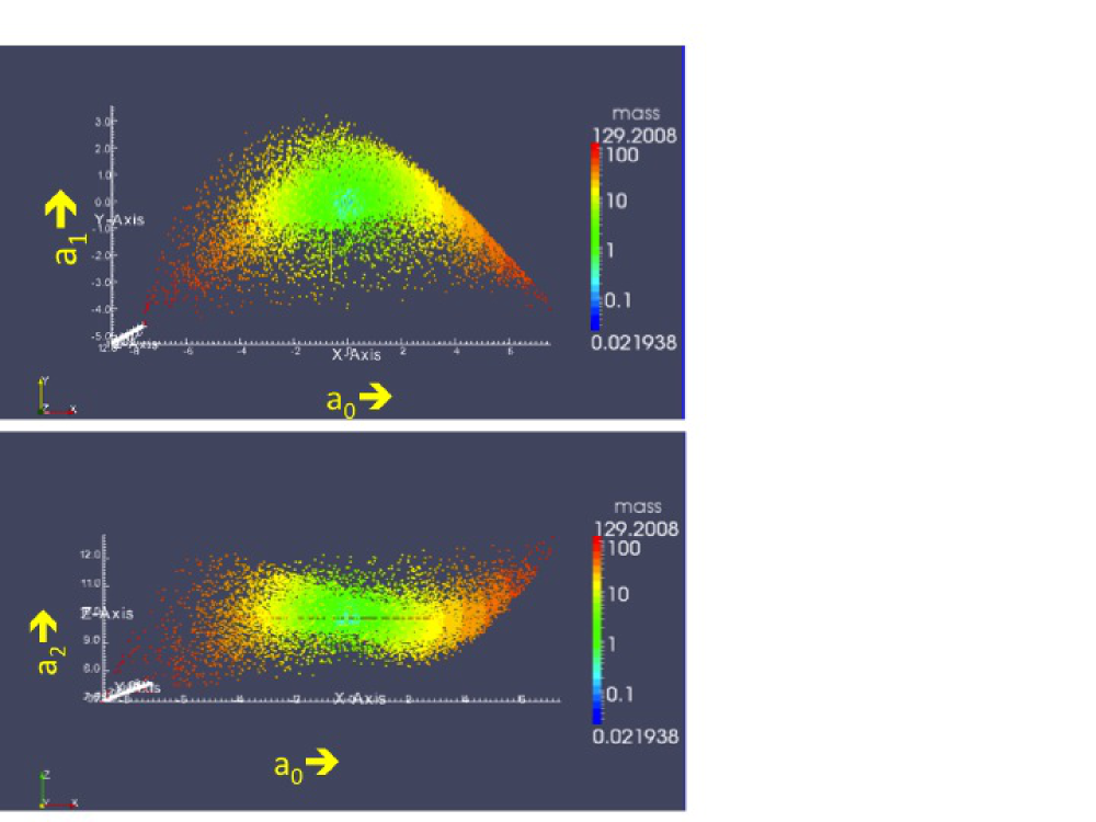
Figure 1: Each galaxy history is a point in the (42 or 20-dimensional) space spanned by $PC_{n}$. For all galaxies in the Millennium $M_{\star}(z=0)\sim 3\times 10^{10}M_{\odot}$ sample, our fiducial sample, we show $PC_{n}$ components in the first three dimensions (these dimensions have the largest spread in values). We take $x,y,z$ to correspond to the directions $PC_{0},PC_{1},PC_{2}$, so $a_{0}$ is shown along the $x$-axis, $a_{1}$ along the $y$-axis, and $a_{2}$ along the $z$-axis. The $(a_{0},a_{1})$, i.e., $(x,y)$ plane is shown in the top panel, and the $(a_{0},a_{2})$, i.e., $(x,z)$ plane in the bottom panel. The colour (“mass”) indicates $\Delta M^{2}=\sum_{n=0}^{41}a_{n}^{2}\times(10^{10}M_{\odot})^{2}$, with average 8.6 $\times(10^{10}M_{\odot})^{2}$ and median 4.6 $\times(10^{10}M_{\odot})^{2}$. The direction of $PC_{0}$ has the largest variance by construction. The distribution of $a_{0}$ and of the signed fractional contribution to each galaxy’s $\Delta M^{2}$, $\alpha_{0}$, are shown for this sample in Fig. 7. As can be seen, the range of $a_{0}$ is much larger than that of $a_{1}$ or $a_{2}$, i.e. $PC_{0}$ dominates, and although the shape is not Gaussian in each direction, the fact that the coefficients do tend to be near their central value is visible as well.

Fig. 1 shows $a_{0},a_{1},a_{2}$ for the $\sim 19,000$ stellar mass histories of Millennium sample galaxies with $M_{\star}(z=0)\sim 3.0\times 10^{10}M_{\odot}$. This set of galaxies will be our fiducial sample for examples below. In Fig. 1, the colour corresponds to the full $\Delta M^{2}$:

$$\Delta M^{2}=\sum_{n=0}^{41}a_{n}^{2}\times(10^{10}M_{\odot})^{2}\;,$$ (5)

a rewriting of Eq. 2. That is, $a_{0},a_{1},a_{2}$ are directly visible, while the colour includes the size of the remaining contribution from $a_{3},...,a_{41}$. The median $\Delta M^{2}$ is $4.6\times(10^{10}M_{\odot})^{2}$, while its average is $\sum_{n}var(n)\times(10^{10}M_{\odot})^{2}=8.6\times(10^{10}M_{\odot})^{2}$. Its distribution has a long tail, as seen by the “mass” range in Fig. 1. The average $\Delta M^{2}/M_{\star}^{2}(z=0)$ is shown in Table 1 for all samples.

The rewriting in Eq. 4 holds for any change of basis, not just the $PC_{n}$ chosen to diagonalize the covariance matrix. However, because the $PC_{n}$ are principal components, the $a_{n},a_{m}$ have zero covariance for $m\neq n$, $\langle a_{m}a_{n}\rangle=\delta_{nm}\,var(n)$. A quantity we will also use later is the signed fraction of $\Delta M^{2}$ due to $PC_{n}$ for a given galaxy, i.e.

$$\alpha_{n}\equiv sign(a_{n})\frac{a_{n}^{2}\times(10^{10}M_{\odot})^{2}}{\Delta M^{2}}\;.$$ (6)

The $\alpha_{n}$ indicate how much each particular $\pm PC_{n}$ contributes to a galaxy’s $\Delta M^{2}$, its separation from the average history. A galaxy with $\alpha_{0}=1$ for instance, is proportional to $PC_{0}$, but can have an arbitrary $\Delta M^{2}$ ($\propto a_{0}^{2}$) from the average history.

Tracking issues motivated us to modify the above procedure for the OWLS stellar mass histories. The stellar masses of Millennium galaxies do not decrease between time steps, however in the OWLS models, 75% of the AGN+SN and 50% of the SN only histories had stellar mass loss at one or more step, and 49/800 (AGN+SN) and 18/800 (SN only) galaxies lost over half of their mass between two consecutive steps. This latter huge mass loss seems to be due the way stellar mass is assigned to galaxies when a galaxy changes from a central to a satellite galaxy and back again. We dropped these histories with the most extreme mass loss (i.e. 50 per cent or more) in computing and ordering the principal components, but then included all galaxies to calculate the variance due to each principal component. (This occasionally leads the fraction of variance due to a $PC_{n}$ to increase with $n$.)

For the Millennium samples, we also briefly compare PCA results for stellar mass histories with their counterparts for galaxy halo histories, star formation rate histories and specific star formation rate histories. We modified how we applied PCA for these histories in the following ways and for the following reasons. A first change is that these other histories are not rescaled to be identical at $z=0$. The rescaling of stellar mass histories to get the same $z=0$ stellar mass in each sample was to remove the effects of finite bin size in our samples, i.e. fluctuations due to slight changes in final stellar mass. In contrast, for each essentially fixed final stellar mass sample, the differences in final halo masses, star formation rates and specific star formation rates are all physical properties of interest. A second change was the use of logarithms for halo mass. As halo histories have a very large spread in final halo mass values, those with large final mass heavily dominate the principal components. This is somewhat improved by using $\log_{10}M_{\rm halo}$. (In part this difficulty did not arise for stellar mass because we worked with samples sharing essentially the same final stellar mass. We could have used $\log_{10}M_{\star}$ for stellar mass histories as well, but chose not to because it tends to emphasize the early times of histories which are more sensitive to resolution effects and less related to final time observables of interest to us.) In addition, halo mass histories for galaxies which switch from central to satellite and back again, or are more than 3 times the root mean square $\Delta(\log_{10}M_{\rm halo}/h^{-1}M_{\odot})$ from the median are excluded when finding the halo bases $PC_{n,{\rm halo}}$ in order for the components to represent most of the histories rather than the large remaining outliers. We include all haloes when calculating the $PC_{n,{\rm halo}}$ contributions to the variance. This leads to the non-monotonic behaviour with $PC_{n,{\rm halo}}$ seen for some of the $n$ values in Fig. 4 below. Another subtlety of halo histories is that, in simulations, the halo mass of a satellite is fixed to be the halo mass right before it became a satellite. These constant satellite halo masses and the fact that some galaxies switch from central to satellite and back several times tend to complicate interpretation. As a result, while we will mention some results below, we will not consider these histories in as much depth as the stellar mass histories. Note that Wong and Taylor (2011) considered halos rather than galaxy halos and thus did not encounter these issues, which are associated with subhalos, not halos.

3 PCA Classification

We now discuss the properties of the PCA classification of the galaxy stellar mass histories. As PCA concerns fluctuations around the origin in a 42 or 20-dimensional space for our samples, for each sample we start by showing the origin (the average stellar mass history). We then turn to the shape of each sample’s distribution around the origin ($var(n)$ of each of the $PC_{n}$), touching upon the $PC_{n}$ contributions for the halo mass, star formation rate and specific star formation rate counterparts. We comment briefly on the accuracy of approximating galaxy histories with a certain number of $PC_{n}$ (covered in more depth in the Appendix), and the properties of the $PC_{n}$, and $PC_{0}$ in particular, as functions of time.

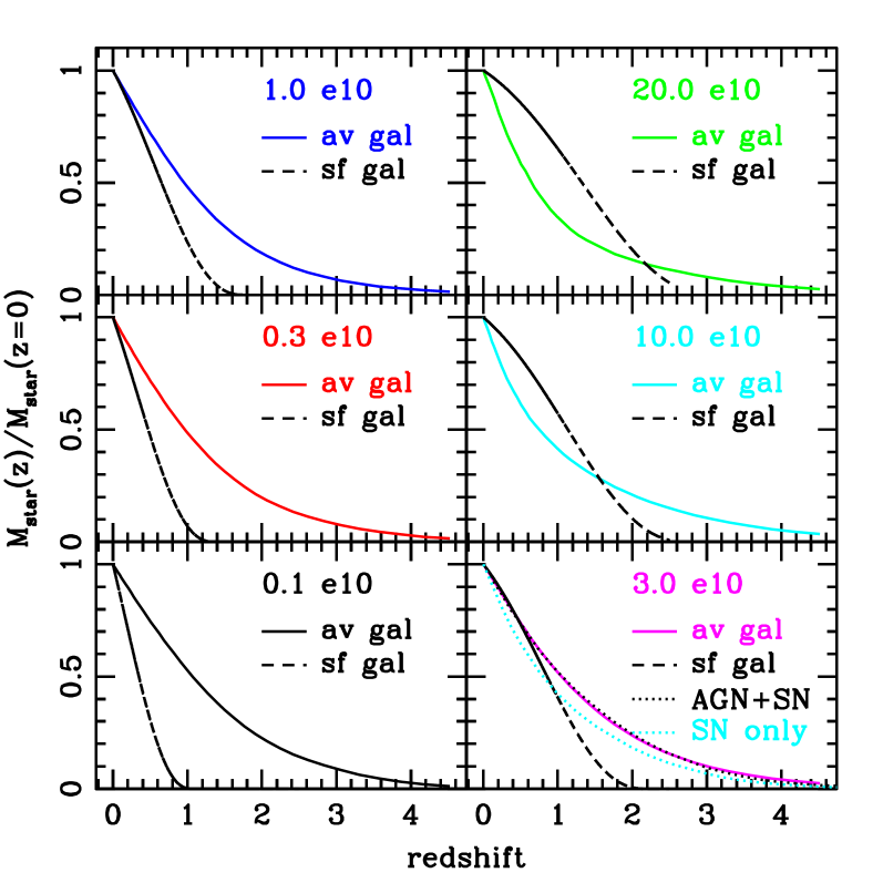
Figure 2: Average histories for the 8 final stellar mass samples, rescaled to final stellar mass of each sample (solid lines for Millennium, dotted for OWLS) in order to highlight similarities and differences between them. Shown as well (dashed lines) is the history of a galaxy with the same final mass on the observationally inferred star-forming main sequence from Leitner (2012). For high final stellar mass galaxies, the average stellar mass growth is often higher at late times than that of a galaxy on the star forming main sequence.

The average histories for all samples are shown in Fig. 2, rescaled by their final stellar mass to allow easier intercomparison. These curves are each the origins in their respective (42 or 20-dimensional) spaces spanned by their PCA $PC_{n}$. Also shown, for reference, are the corresponding stellar mass histories of galaxies on the star forming main sequence with the same final stellar mass, inferred from observational data and using different assumptions than the simulations, by Leitner (2012) (amended Eq. A3, shown in his Fig. 9). The average histories for the two higher final stellar mass samples grow more quickly at late times than a galaxy on the star forming main sequence, presumably due to higher than main sequence star formation rates, stellar mass gain through mergers, or some difference between the Millennium models and the assumptions for the inferred histories from observation. These two higher final stellar mass bins also exhibit other differences in their histories from those with lower stellar mass, as will be seen later.

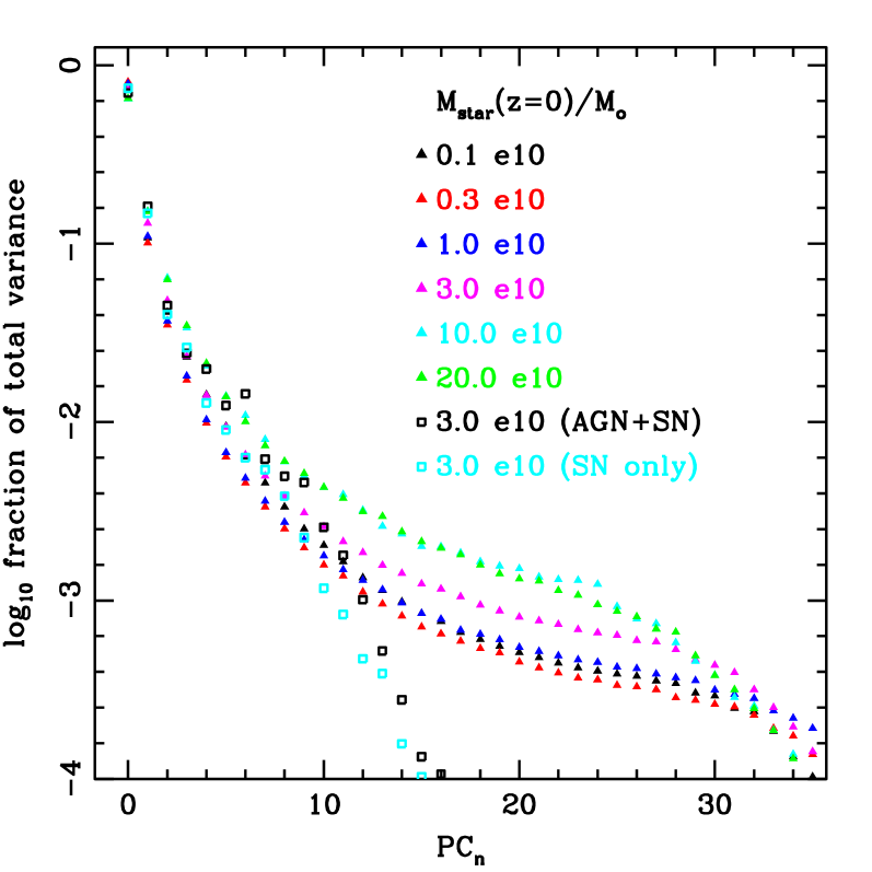
Figure 3: Logarithm of the fraction of the total variance $var(n)/\sum_{m}var(m)$ due to $PC_{0}$, $PC_{1}$, up to $PC_{35}$, for the 6 Millennium samples, ($M_{\star}(z=0)/M_{\odot}\sim$ $10^{9},3\times 10^{9},10^{10},3\times 10^{10},10^{11},2\times 10^{11}$), and the two OWLS samples ($M_{\star}(z=0)/M_{\odot}\sim 3\times 10^{10}$), with colours as in Fig. 2. There are fewer outputs for the OWLS runs, hence fewer $PC_{n}$. Contributions to the variance around the average histories (shown in Fig. 2) quickly drop to below a percent after the first few $PC_{n}$.

The fraction of the variance $var(n)$ due to each $PC_{n}$ characterizes the ensemble of stellar mass histories. As seen in Table 1 and Fig. 3, the leading three $PC_{n}$ contribute a significant fraction, $\sim 90\%$, of the total variance around the average history, with $PC_{0}$ strongly dominating (note that the y-axis is logarithmic). For the Millennium histories this means the remaining $\lesssim 10\%$ of the variance is split among the remaining 39 $PC_{n}$, for the OWLS histories this fraction of the variance is shared amongst the remaining 17 $PC_{n}$. The predominance of $PC_{0}$ is also indicated in Fig. 1 by the much larger range of values for the $a_{0}$ distribution, relative to $a_{1}$ and $a_{2}$.

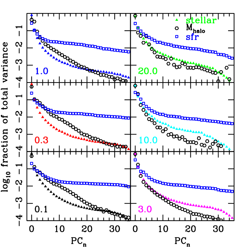
Figure 4: Logarithm of the fractional variance due to each corresponding PCA component for stellar mass (solid triangles), $\log_{10}M_{\rm halo}$ (open hexagons, black) and star formation rate (open squares, blue) histories, for all 6 Millennium samples. The stellar mass histories are the same as in Fig. 3, they and the halo mass histories are dominated by the first few components, while those for star formation rate require a large number of components to describe the same fraction of total variance around the average history. $M_{\star}(z=0)/10^{10}M_{\odot}$ is at lower left in each panel.

For some context and comparison, Fig. 4 shows the principal component contributions for the Millennium stellar mass histories of Fig. 3 again, but now alongside their counterparts for the star formation rate and $\log_{10}M_{\rm halo}$ (as described earlier, recall $\log_{10}M_{\rm halo}$ is used due to the large halo mass range) for the same samples. The star formation rate histories are not dominated by the first few principal components: on average less than half of the total variance is due to the first three $PC_{n,{\rm sfr}}$. In contrast, just as for the stellar mass histories, the halo mass histories are strongly dominated by the first few principal components. On average 87 per cent of the total variance is due to the first three $PC_{n,{\rm halo}}$. This fraction of the variance changes noticeably with sample, perhaps in part due to differences in their satellite fractions (Table 1). Again, the scatter up and down for $PC_{n,{\rm halo}}$, especially apparent in the highest mass samples, happens because the $PC_{n,{\rm halo}}$ are calculated (and assigned an order) with a subset of the galaxies, as described at the end of §2.2, while the full set of galaxies is used to compute their variance contributions.

We also considered the specific star formation rate (not shown for brevity). Its principal component fractional contributions to the variance fall between those for star formation rate and stellar mass in Fig. 4, with the first three components contributing on average 3/4 of the variance. For higher $n$ components, the specific star formation rate contributions are close to those for $\log_{10}M_{\rm halo}$ for the three lowest final stellar mass samples ($M_{\star}(z=0)<3\times 10^{10}M_{\odot}$). For $M_{\star}(z=0)\geq 3\times 10^{10}M_{\odot}$, the higher $n$ specific star formation rate principal components contributions tended to be much higher than for $\log_{10}$ halo mass. For all final stellar mass samples, the fraction of the variance due to the $n$th principal component for specific star formation rate drops below that for stellar mass around $n=20-22$.

In addition to studying contributions to the total scatter of the sample, the $var(n)$, one can also ask about contributions to individual galaxy histories, in particular how well keeping only a small number of $PC_{n}$ modes in the expansion shown in Eq. 4 approximates individual galaxy stellar mass histories. Once a galaxy stellar mass history is approximated by about 20 $PC_{n}$, 95% of galaxies are within $<0.15M_{\star}(z=0)$ of their true history, and within 10% of their true $\Delta M^{2}$. See the Appendix for figures showing more detailed trends for how these approximations work as final stellar mass and number of $PC_{n}$ are varied.

We now turn to the $PC_{n}$ themselves as functions of redshift. The leading three $PC_{n}$ for the fiducial sample (where they account for 91% of the variance) are shown in Fig. 5. Again, this is the Millennium $M_{\star}(z=0)\sim 3\times 10^{10}M_{\odot}$ sample. The coefficients of each are set to their median positive (for $+PC_{n}$) or negative (for $-PC_{n}$) values. The $n$th $PC_{n}$ crosses zero $n$ times. For the highest $PC_{n}$, there is a lot of “ringing” at the highest redshifts, with large amplitudes (but with small coefficients $a_{n}$).

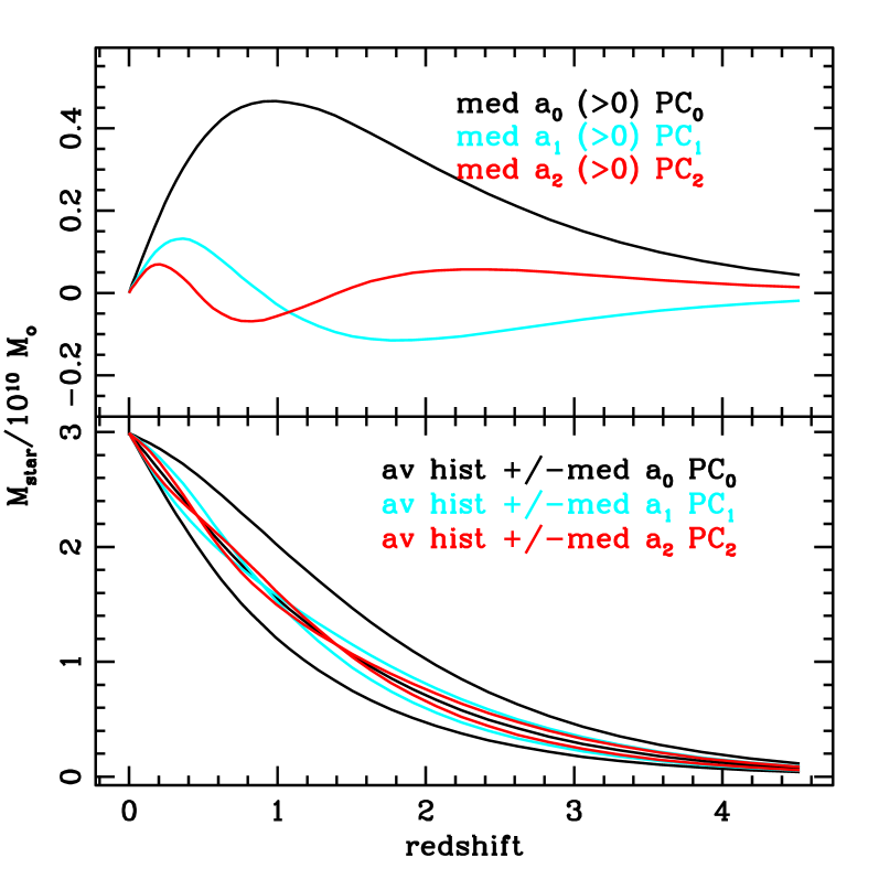
Figure 5: Dominant paths contributing to fluctuations around the average galaxy stellar mass history, for galaxies in the fiducial (Millennium $M_{\star}(z=0)=3\times 10^{10}M_{\odot}$) sample. Top: the three most dominant PC’s, multiplied by their respective median positive coefficients $a_{0},a_{1},a_{2}$. Bottom: the fluctuations added to the average history, with positive and negative coefficients set to their respective median values for the fiducial sample.

The extrema are spaced more regularly in lookback time than in redshift. Regularity was also seen by Wong and Taylor (2011) when using the scale factor $a$ as time coordinate for their halo history principal components. They mentioned the similarity to Fourier modes, although unlike Fourier decomposition, with the PCA expansion both the coefficients and the basis components (i.e. basis modes) are determined by the sample.

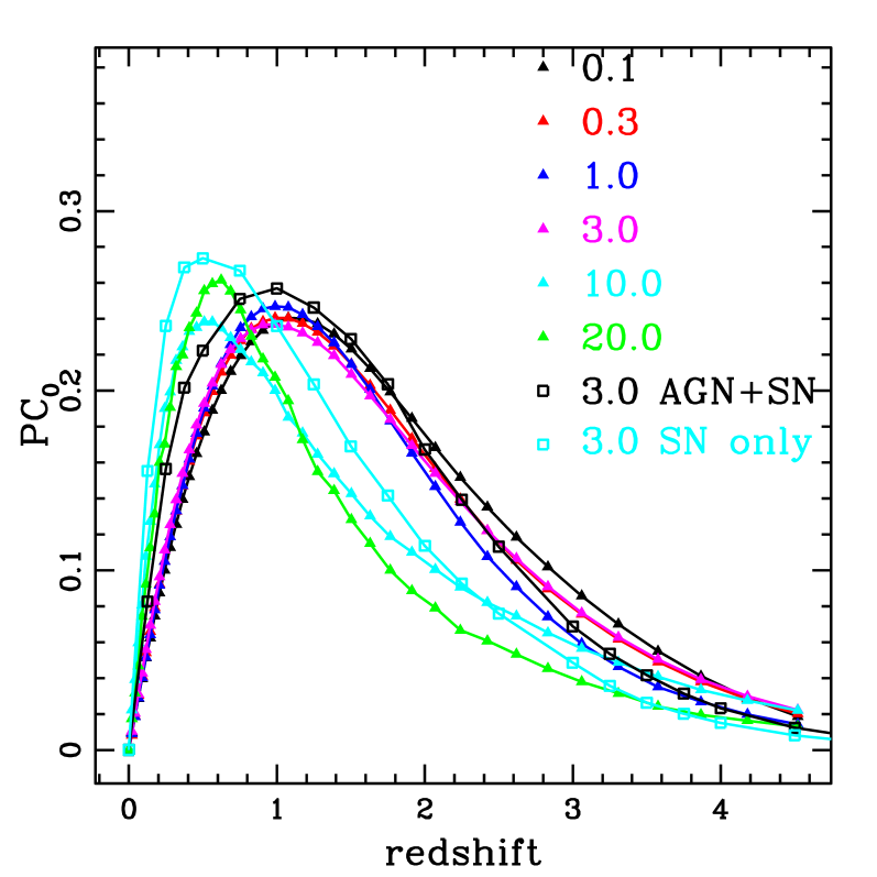
Figure 6: The normalized (for Millennium) leading fluctuation around the average galaxy stellar mass history, $PC_{0}$, for all 8 samples, colours as in Fig. 3 (listed in terms of $M_{\star}(z=0)/10^{10}M_{\odot}$ as well). The two OWLS $PC_{0}$ are normalized to length $\sqrt{20/42}$ to compensate for the smaller number of output times. The $PC_{0}$ for the four lowest $M_{\star}(z=0)$ Millennium samples and the AGN+SN OWLS samples have inner product $>0.99$ with each other, similarly for the two highest $M_{\star}(z=0)$ Millennium samples and the SN only OWLS sample. When one $PC_{0}$ is taken from both groups the overlap is smaller, dropping to 0.91. In the Millennium sample, there seems to be a qualitative change above $M_{\star}(z=0)=3\times 10^{10}M_{\odot}$. The triangles and squares show the actual output times of the simulations (which imply a certain weighting of different periods of time for the PCA analysis).

The leading component, $PC_{0}$, dominates the variance, and as will be seen below, many of the individual galaxy histories as well. Fig. 6 shows $PC_{0}$ as a function of redshift for all 8 samples. The data points are the simulation output redshifts, whose spacing provides an implicit weighting for $\Delta M^{2}$. To allow easier visual comparison between $PC_{0}$ for the OWLS and Millennium models, we multiplied $PC_{0}$ for OWLS by $\sqrt{20/42}$, to compensate for its smaller number (20) of output times compared to Millennium (42).

We see that although $PC_{0}$ is dominant and has a single peak in all cases, differences appear as final stellar mass and simulation are varied. The smoothness of the leading $PC_{n}$, in particular $PC_{0}$, allows us to use linear interpolation to intercompare them between simulations with different numbers of output times. $PC_{0}$ is similar amongst the four lowest $M_{\star}(z=0)$ Millennium samples and the AGN+SN OWLS sample, as well as amongst the two higher $M_{\star}(z=0)$ samples and the SN only OWLS sample. Within these groups inner products are $>0.995$, but between the two groups they can drop to 0.91. The notable feature in $PC_{0}$ is its peak, which is at lower redshift for the two highest $M_{\star}(z=0)$ Millennium samples and the SN only OWLS sample, but at approximately the same redshift for the lower $M_{\star}(z=0)$ samples and the AGN+SN OWLS sample. The two OWLS samples share the same final stellar mass as the fiducial sample, one of the lower $M_{\star}(z=0)$ samples. The difference between the two OWLS samples is probably due to overcooling in the SN only case, leading to too much late time star formation as compared to observations. (The source of the difference between higher and lower final stellar masses is less clear, but possibly related to the increased importance of mergers for the former.) Thus we see how the behaviour of $PC_{0}$ discriminates between families of histories with different physics and (sometimes) with different final stellar mass.

In summary, $PC_{0}$ dominates the stellar mass histories for all the different samples, and the first three $PC_{n}$ capture $\sim$90% of the variance of the full sample. In addition (see Appendix for further discussion), a large fraction of individual galaxy stellar mass histories can be well approximated by a subset of the $PC_{n}$. The leading $PC_{0}$ has one feature, a peak, and is similar for the $M_{\star}(z=0)\leq 3\times 10^{10}M_{\odot}$ Millennium samples and the AGN+SN OWLS sample. A different $PC_{0}$ seems to be shared between the two higher $M_{\star}(z=0)$ Millennium samples and the SN only OWLS sample, peaking at a lower redshift. The halo history (which is somewhat more difficult to interpret) PCA shows similar dominance of the leading few components, while that for the specific star formation rate histories is slightly weaker. Star formation rate histories require many more principal components to get a similar fraction of the variance compared to the stellar mass case.

4 PCA classification and other galaxy properties

The PCA decomposition revealed that a few parameters characterize a large fraction of the total deviation from the average stellar mass history for the ensemble of histories, and that a large fraction of each galaxy’s history is captured by the leading $PC_{n}$. We now look for relations of the PCA characterizations with other galaxy properties, in particular their halo histories, specific halo and stellar mass history times, and observables at a fixed time (in our case $z=0$).

We start with $\alpha_{0}$, the fraction of a galaxy’s history due to $\pm PC_{0}$, where $\alpha_{0}>0$ corresponds to a $PC_{0}$ contribution with earlier stellar mass gain than the average history, and $\alpha_{0}<0$ to later stellar mass gain than the average history.

One interesting history to consider in terms of the leading fluctuation, $PC_{0}$, is the observationally derived history of a galaxy on the star forming main sequence (Leitner (2012), shown in Fig. 2), for a given final stellar mass. We can write this history in terms of $a_{n}$ for each sample, and calculate its corresponding $\alpha_{0}$, which additionally quantifies the fractional contribution of $PC_{0}$ to any history’s $\Delta M^{2}$. We find $\alpha_{0}=$ (-0.94,-0.97, -0.89, -0.54, +0.55, +0.89) for Millennium $M_{\star}(z=0)=$(0.1, 0.3, 1.0, 3.0, 10.0, 20.0 $\times 10^{10}M_{\odot}$) and (-0.54, -0.02) for OWLS (AGN+SN, SN only, both with $M_{\star}(z=0)=3.0\times 10^{10}M_{\odot}$). That is, the star forming main sequence corresponds to $\alpha<0$, late stellar mass gain, for the lowest final stellar mass histories in Millennium and the AGN+SN OWLS sample. This special history is in fact predominantly (contributing more than 90 percent of $\Delta M^{2}$) along the direction of $-PC_{0}$ for the two lowest final stellar mass histories in Millennium. For the two highest final stellar mass histories in Millennium, the Leitner (2012) observationally derived star forming main sequence has slower stellar mass growth than the average history, and actually corresponds to early stellar mass gain in terms of $PC_{0}$ ($\alpha_{0}>0$). It may be that for these galaxies late stellar mass gain is due to mergers (which are more common for their likely hosts, halos with large masses, which also tend to have less star formation), starbursts, or perhaps some difference between the theoretical modeling and the inferences from observations.

Considering other galaxy stellar mass histories, one might guess that early stellar mass gain relative to the average history, $\alpha_{0}>0$, corresponds to a quiescent galaxy, for instance a quenched satellite. (Quenched central galaxies may be expected to have relatively more late stellar mass gain from mergers.) Consistent with this, for the lower stellar mass Millennium samples, satellites are an increasing fraction of the galaxies as $\alpha_{0}$ increases from negative to positive. Similarly, $\alpha_{0}<0$, i.e. late stellar mass gain relative to the average history, is more common for low final stellar mass centrals and this trend reverses as $M_{\star}(z=0)$ increases. The interpretation is less clear for the two higher final stellar mass samples, which have $\alpha_{0}>0$ for the star forming main sequence, and satellites which are either a constant or decreasing fraction of the galaxies as $\alpha_{0}$ increases.

Figure 7: Left: distribution of $a_{0}$, the coefficient of $PC_{0}$ in a galaxy’s history, for the fiducial (Millennium $M_{\star}(z=0)=3\times 10^{10}M_{\odot}$) sample. The distribution of $a_{0}$ is asymmetric and narrower than a Gaussian (dotted line) with the same $\sigma(=2.5)$ and normalization. Right: distribution of the signed fraction of each individual galaxy’s total variance $\Delta M^{2}$ due to $PC_{0}$, $\alpha_{0}$, which is positive or negative depending upon whether the galaxy has $\pm PC_{0}$ in its history, again for the fiducial sample. An $\alpha_{0}=1$ galaxy has all of its deviation from the average history made up of $+PC_{0}$.

The fractions of galaxies with $\alpha_{0}<-0.5$ and $\alpha_{0}>0.5$, respectively “lowpc”/“highpc”, are listed for all 8 samples in Table 1. These are galaxies where at least half of their $\Delta M^{2}$ is due to $PC_{0}$, i.e. to the simple shaped fluctuation in Fig. 6 determined separately for each sample. For a multivariate Gaussian with the same variances as our fiducial model there would be 2/5, 1/5, 2/5 of the sample in the regimes $\alpha_{0}\in$ [-1,0.5),[-0.5,0.5],(0.5,1]. In comparison, for our samples there are relatively more galaxies in the central regions; in addition, the high and low $\alpha_{0}$ regions are not symmetric. The $\alpha_{0}$ distribution for all galaxies in the fiducial sample is shown in the right panel of Fig. 7, where peaks at $\alpha_{0}=\pm 1,0$ are visible, characteristic of a dominant $PC_{0}$ in a many dimensional system.

Because halo mass history variances are also often dominated by $PC_{0,{\rm halo}}$ (in fact slightly more so than the stellar mass history variances by $PC_{0}$, for the three highest final stellar mass samples), one might expect that many galaxies have sizable contributions from $PC_{0,{\rm halo}}$ in their individual histories. In terms of the analogue of $\alpha_{0}$ for halo mass histories, $\alpha_{0,{\rm halo}}$, defined via $a_{0,{\rm halo}}$ as in Eq. 6, we found $|\alpha_{0,{\rm halo}}|>0.5$ for (52%, 56%, 24%, 68%, 69%, 55%) of the Millennium galaxies. (This can be compared to the stellar mass history counterpart, the sums of “highpc” and “lowpc”, in Table 1.) That is, for all but one final stellar mass sample, a large fraction of galaxies have more than half of their $(\Delta\log_{10}M_{\rm halo})^{2}$ along the $PC_{0,{\rm halo}}$ direction. The $M_{\star}(z=0)=10^{11}M_{\odot}$ sample is likely an outlier because its $PC_{0,{\rm halo}}$ direction is associated with a low fraction, 42%, of the total variance, as compared to the average fraction for the other samples ($\sim 2/3$). In addition, $\alpha_{0,{\rm halo}}$ is also often strongly correlated with $\alpha_{0}$, with correlation coefficients (73%, 68%, 65%, 64%, 19%, 54%). In the OWLS models the correlations between $\alpha_{0}$ and $\alpha_{0,{\rm halo}}$ was roughly 1/3 in both cases; stellar mass history and halo mass history seemed less correlated in the two hydrodynamical simulations by this measure. This quantity would be interesting to compare in other simulated samples, although as noted earlier, issues of how halo mass is defined for a galaxy when it becomes a satellite (fractions are shown for our samples in Table 1) and satellite to central switches generally make interpretation of the halo histories more challenging. Relations between average halo mass and stellar mass and/or (specific) star formation rate have been derived observationally at fixed redshift (e.g. Vale & Ostriker, 2006; Conroy, Wechsler & Kravtsov, 2006; Moster et al., 2010; Leauthaud et al., 2011; Reddick et al., 2013) and relations have also been found on average between stellar mass and halo mass growth (More et al., 2009; Yang, Mo and van den Bosch, 2009; Yang et al., 2012; Behroozi, Wechsler & Conroy, 2013a, b; Hudson et al., 2013; Moster, Naab & White, 2013; Tinker et al., 2013; Wang et al., 2013).

4.1 Correlations with history times

Going beyond correlations with $\alpha_{0,{\rm halo}}$, we searched for further relations between stellar mass PCA quantities and theoretical and observational properties. In principle such relations might differ between simulations, however, as many quantities in the OWLS models were not defined in the same way, we focus on the Millennium samples only. The PCA description quantities we considered were $a_{0}$, $\alpha_{0}$, $\alpha_{1}$, $\alpha_{2}$, $\Delta M^{2}$ and $\Delta M_{+}^{2}=\sum_{m=3}^{N}a_{m}^{2}\times(10^{10}M_{\odot})^{2}$. We will show mostly results for $a_{0}$ below, others will be mentioned for the cases where we found large correlations. The $a_{0}$ for a galaxy is the total amount of its history due to $PC_{0}$, rather than the signed fractional contribution to $\Delta M^{2}$ measured by $\alpha_{0}$. We use $a_{0}$ for these comparisons because dependence upon $\alpha_{0}$ has much more structure due to the three peak distribution of $\alpha_{0}$, visible in Fig. 7. (Often the correlation coefficients for $a_{0}$ and $\alpha_{0}$ are very similar, some examples are given of this below.)

We first consider the relation between $a_{0}$ and several times which characterize galaxy stellar mass or halo mass histories. Unlike the $PC_{n}$ coefficients, these times do not say anything about the shape of the stellar mass history or the halo mass history aside from the time it reaches a certain value. For stellar mass history times, we take the redshifts $z_{10},z_{50},z_{90}$ where a galaxy reaches 10%, 50% or 90% of its final stellar mass (if the redshift is before $\sim$ 4.8, the earliest redshift we have, we set it to 5). For halo history we take times which have been used to identify which galaxies might be quiescent in the “age matching” model of Hearin & Watson (2013). These are:
$z_{12}$: the redshift at which the galaxy’s halo mass $M_{vir}$ reaches $10^{12}h^{-1}M_{\odot}$.
$z_{\rm grow}$: the redshift when a galaxy’s halo growth falls below a certain rate. We take the definition of Wechsler et al. (2002) as suggested by Hearin & Watson (2013); Hearin et al. (2013b), $d\log M_{\rm halo}/d\log a\equiv\Delta\log M_{\rm FoF}/\Delta\log a<2$.
$z_{\rm infall}$: The redshift when a galaxy falls into another halo and becomes a satellite.
$z_{\rm starve}$: The earliest redshift of $z_{12},z_{\rm grow},z_{\rm infall}$.
Subhalo times are used if the galaxy is a satellite. Two other previously discussed PCA history quantities are also included, $\Delta M^{2}/M_{\star}(z=0)^{2}$, the total squared deviation of a particular galaxy’s history from the average, and $\alpha_{0}$, the fractional contribution to a galaxy’s $\Delta M^{2}$ due to $PC_{0}$.

The distributions of these quantities relative to $a_{0}$ are shown at the top panel of Fig. 8, for the fiducial sample. Correlation coefficients are shown in each panel in the upper left corner. In the bottom panel we show the correlation coefficients again, along with their counterparts for the other 5 Millennium samples, to illustrate trends with changing final stellar mass. Lines are drawn at $\pm 40\%$ to draw attention to large positive and negative correlations.

Many of the correlations are large. The large correlation of $a_{0}$ with the times $z_{10},z_{50},z_{90}$ is not surprising, as $a_{0}$ corresponds to a component of a galaxy’s history with early (for a positive sign) or late (for a negative sign) stellar mass gain, and $PC_{0}$ dominates the history of many of the galaxies (Fig. 7). The PCA description goes beyond these specific times in a galaxy’s stellar mass history to say how much of that history’s departure from the average is due to a particular shape, i.e. due to $PC_{0}$.

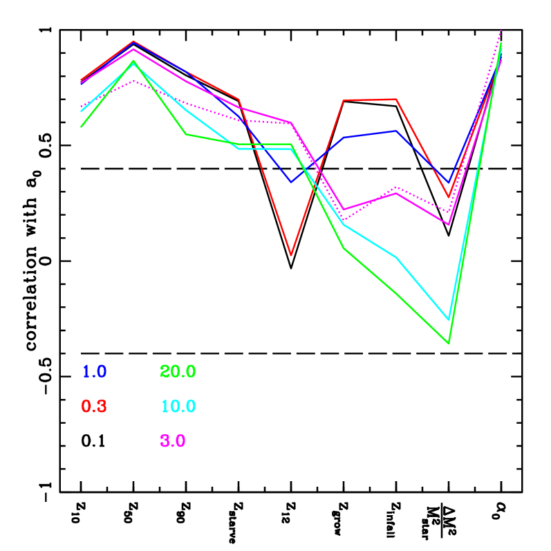
Figure 8: Comparison of $a_{0}$ with other galaxy history characterizations. Top: For the fiducial sample, distributions of the leading PCA coefficient, $a_{0}$, versus several halo history and stellar mass history quantities. Bottom: The correlation coefficients for the above scatter plots and their counterparts for all 6 Millennium samples. Coloured curves are for different final stellar mass samples, as indicated in the legend in terms of $M_{\star}(z=0)/10^{10}M_{\odot}$ in the lower left corner. The dotted line is the correlation coefficient for $\alpha_{0}$, rather than $a_{0}$, i.e. the signed fractional contribution to $\Delta M^{2}$ from $PC_{0}$, for the fiducial sample. The times $z_{10}$, $z_{50}$, and $z_{90}$ are when galaxies have reached 10%, 50% and 90% of their final stellar mass, while the halo history times $z_{\rm starve}$, $z_{12}$, $z_{\rm grow}$ and $z_{\rm infall}$ have been suggested as determining the “age” of a galaxy. See text for definitions. The measure $\Delta M^{2}$ is total “distance” squared of a galaxy’s stellar mass history from the average, and $\alpha_{0}$ is the signed fraction of a galaxy’s $\Delta M^{2}$ due to $PC_{0}$. Strong correlations are present for many of the characteristic redshifts.

A strong correlation with $z_{starve}$ is also not unexpected, as earlier $z_{starve}$ means earlier shut off of star formation, which again (given that all galaxies in each subsample have the same final stellar mass) leads to the expectation of large positive $a_{0}$ (early stellar mass gain). The higher final stellar mass samples often have weaker correlations of these times with $a_{0}$, which is likely a combination of $a_{0}$ not being as dominant (for all measurements) and star formation perhaps not being as major a component of stellar mass gain. Some other differences for different final stellar mass samples are easy to interpret, e.g. the lower final stellar mass samples rarely reach halo masses large enough to have $z_{12}\neq 0$.

In terms of other PCA related quantities, the correlations with $\alpha_{0}$ are similar, as an example the fiducial sample’s $\alpha_{0}$ correlations are shown as the dotted curve in Figs. 8 and 9. Correlations with $\alpha_{1},\alpha_{2}$ are relatively small, except for the subsamples with $\alpha_{1}>0.5$ or $\alpha_{2}>0.5$ respectively (not shown). For these the large correlations which appeared were strongly $M_{\star}(z=0)$ dependent. As can be seen, as $a_{0}$ increases, the scatter $\Delta M^{2}$ from the average history tends to increase for the four lower final stellar mass samples, and decrease for the two highest.

4.2 Correlations with final time observables

We now turn to relations between $a_{0}$ and several $z=0$ observables, to explore the relation between PCA characterizations of stellar mass histories and possible fixed time measurements. For final time observable quantities, we took $\log_{10}M_{\rm halo}$, $\log_{10}M_{\rm host}$ (for a satellite this is the mass of the main halo in which it is a satellite, rather than its subhalo mass), star formation rate (sfr), g-r colour (SDSS, with dust) and bulge/all stellar mass ratio. These were all calculated or provided directly from the Millennium Guo et al. (2013) database. Scatter plots of these quantities versus $a_{0}$ are shown in the top panel of Fig. 9, for the fiducial sample, and correlation coefficients for all 6 Millennium samples are shown in the bottom panel. The correlation coefficients for $\alpha_{0}$ for the fiducial sample are also shown. The correlations between stellar mass history PCA properties and final time galaxy properties may give clues as to how to estimate stellar mass history properties from fixed time observables.

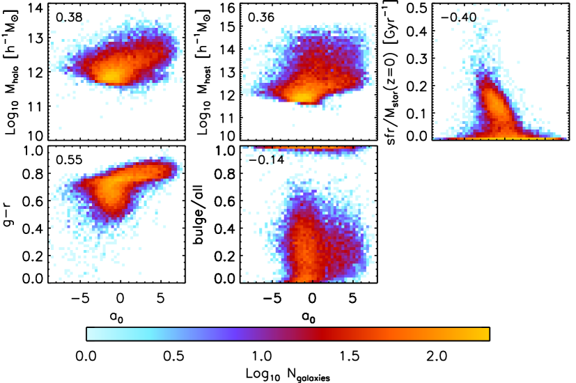
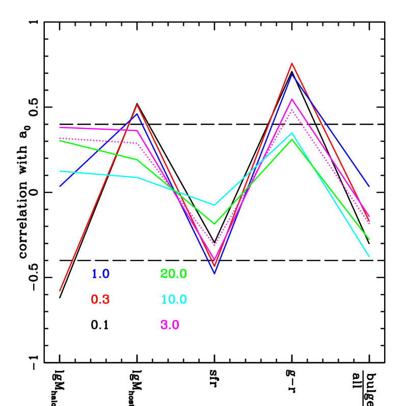
Figure 9: Relation of leading PCA coefficient, $a_{0}$, to final time observable properties. Top: For fiducial sample, distribution of $a_{0}$ relative to $\log_{10}M_{\rm halo}$, $\log_{10}M_{\rm host}$, sfr$/M_{\star}(z=0)^{2}$, $g-r$ colour, and bulge/all stellar mass. Bottom: Correlation coefficients for all 6 Millennium samples, for the same quantity. Coloured curves are for different masses, as indicated in the legend in terms of $M_{\star}(z=0)/10^{10}M_{\odot}$ in the lower left corner. The dashed line is the correlation coefficient for $\alpha_{0}$, rather than $a_{0}$, i.e. the signed fractional contribution to $\Delta M^{2}$ from $PC_{0}$, rather than its value, for the fiducial sample. We find strong correlations with halo and host mass, star formation rate, and colour, especially for low stellar mass bins.

Many large correlations are seen, and often are as expected. For instance, large $a_{0}$ indicates a large early stellar mass gain component and is correlated with larger g-r colour, i.e. redness and lower star formation. For the higher final stellar mass samples, large $a_{0}$ is also correlated with higher halo mass and host halo mass. Again, correlations are weaker for the two highest stellar mass samples, for the reasons given above. For the two lowest final stellar mass samples ($\leq 0.3\times 10^{10}M_{\odot}$), $M_{\rm halo}$ and $a_{0}$ have a negative correlation (satellites cause the correlation between $a_{0}$ and $M_{\rm host}$ to remain positive). For these, then, the higher the halo mass, the later the stellar mass gain, reversing as final stellar mass increases. Another feature (not shown) is that for all but the highest stellar mass sample, a large $\Delta M_{+}^{2}\propto\sum_{m=3}^{N}a_{m}^{2}$ is strongly correlated with a large bulge/all stellar mass ratio.

To summarize, the sign of the contribution to $PC_{0}$ corresponds to a history component with early or late stellar mass growth, and the signed fractional contribution of $PC_{0}$, $\alpha_{0}$, is often large and negative for the observationally derived star forming main sequence in terms of the bases found for the Millennium samples. This fractional contribution and the total contribution $a_{0}$ of $PC_{0}$ in Millennium are both strongly correlated with $z=0$ colour (g-r) and star formation, as well as $z_{\rm starve},z_{50}$ and other galaxy halo and stellar mass history times. Increasing the bulge/all stellar mass ratio often correlated with an increase in the total deviation from the average history not due to the first three $PC_{n}$. Again, differences appeared between the lower four and upper two $M_{\star}(z=0)$ samples, which may be in part related to the fact that $PC_{0}$ is less dominant for the latter.

5 Splitting up the histories

Although smooth trends with $a_{0}$ can be seen in Figs. 8 and 9, it is also clear that a separation into different classes appears when one considers $\alpha_{0}$, the fraction of a galaxy’s total deviation from the average history, $\Delta M^{2}$, due to $PC_{0}$ (Fig. 7). In this case, three populations seem to be present, with trends between the populations implied by the correlations in Figs. 8 and 9. However, splitting up the sample of galaxies according to the $PC_{0}$ contribution implies that galaxies with late stellar mass gain are all related to a form of fluctuation that is the mirror image of those of galaxies with early stellar mass gain (i.e. both proportional to $PC_{0}$).

One can use a more flexible characterization to divide up galaxy histories, by associating each galaxy with one (or more) of several different average paths or classes, rather than with symmetric fluctuations around a single central average history. We considered two ways of finding such paths, mixture models and k-means clustering. These do not assume that different basis histories are “orthogonal” and thus can allow more general basis histories, if preferred by the data. Mixture models model the full distribution (of stellar mass histories, in this case) with a combination of several distributions, each here taken to be the same functional form but with different parameters. We took Gaussian distributions (a common choice) as our basis distributions, each with a different average stellar mass history and different scatters. k-means clustering partitions objects into sets, with each object assigned to the set with the closest centre (in this case the closest average history), but does not assume a form for the distribution of galaxy stellar mass histories around each centre. In both, one has to choose the number of components and provide initial guesses for centres. One then solves iteratively for better centres and corresponding galaxy assignments to each component (and, for mixture models, for improved scatters and weights in the full distribution).

We used mixture models based on the first 20 $PC_{n}$ coefficients $\{a_{n}\}$ (see Appendix for how well this approximation works in the Millennium samples). Mixture models based on $M_{\star}(t_{i})$ tended to become numerically unstable due to the large powers in the 41 dimensional determinant of the Gaussian scatters. The initial paths were taken to be a range of functions of the leading $PC_{n}$. For the k-means clustering, each galaxy history $M_{\star}(t_{i})$ is assigned to the $j$th average path $\mu(t_{i})^{j}$ for which $(M_{\star}(t_{i})-\mu(t_{i})^{j})^{2}$ is the smallest. Using $M_{\star}(t_{i})$ directly was stable for k-means clustering, so we used the full histories (rather than the first 20 $PC_{n}$ coefficients as was the case for the mixture models). The initial $\mu(t_{i})^{j}$, where $j$ runs over the number of components, were chosen randomly from the galaxy distributions; once galaxies are assigned to average paths, the averages are recalculated, and the process reiterated.

Both search methods converge to local solutions, so we checked for robustness by finding the best parameters for 9/10 of the sample (training sample), then testing this solution on the remaining 1/10 (test sample), and repeating this 9 times. We found that increasing the number of average paths tended to increase the likelihood of the test sample, even up to $\sim 13$ basis histories (the only exception was a hint of an upturn in the likelihood for the $10^{11}M_{\star}(z=0)$ sample, in one approximation, with 13 components). However, with increasing numbers of components, the interpretations of the resulting sub-populations became more complicated. Although it is possible that the separate classes might be distinguishing between further galaxy properties, given the relative success of the PCA description (galaxy histories tend to be centred at the average history, with a large fraction of the variance in the first fluctuation), we focussed primarily on the 3 component models for further study.

For the lowest $M_{\star}(z=0)=0.1\times 10^{10}M_{\odot}$ final stellar mass sample, the preferred k-means and Gaussian mixture model average paths coincide for both 3 and 4 components. As final stellar mass increases, the mixture models often find average paths which overlap significantly with each other but have different scatter, suggesting that the Gaussian shape is not optimal (as the procedure is then approximating a distribution with a narrow peak plus a large tail). Associating a galaxy with a large or small width Gaussian seemed a less useful classification than identifying the closest average history, as found using k-means. We thus report the k-means results in more depth below.

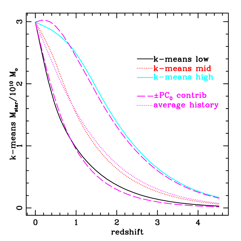
Figure 10: k-means average paths for $M_{\star}(z=0)\sim 3.0\times 10^{10}M_{\odot}$ sample (solid black, dotted red, solid cyan). Also shown are the $\pm PC_{0}$ (top and bottom dashed magenta curves) contributions to the high and low curves and the average history (central dotted magenta curve). These trends occurred for all samples, that is, the three k-means paths are very close to $\pm PC_{0}$ and the average path respectively.

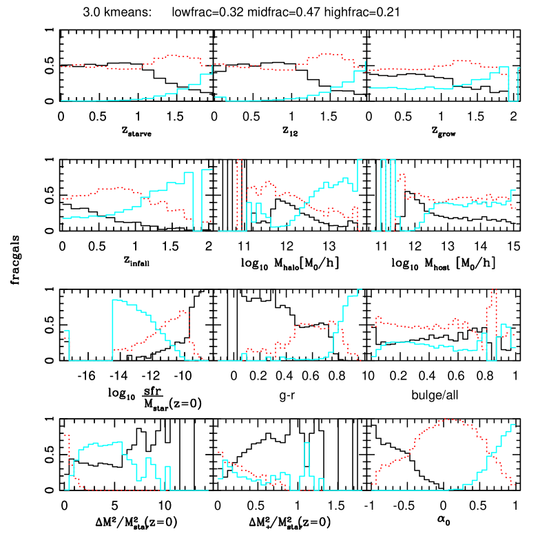
Figure 11: Properties of galaxies in each of the three k-means distributions in Fig. 10; line types and colours of each subsample match that of their corresponding k-means path. Each histogram is the fraction of galaxies in each k-means component, bin by bin (so the sum in any bin of all three components is equal to 1). Properties defined in §4.1 and 4.2, similar to Figs. 8 and 9 (star formation rate is shown logarithmically and, when zero, shown as $<-16$). This indicates how well a given individual final time observation or halo history time can be used to infer to which k-means set a galaxy is likely to belong.

For the fiducial sample, the 3 component k-means average histories are shown in Fig. 10. The black solid, red dotted, and cyan solid lines correspond to the k-means average paths, the $\mu(t_{i})^{j},j=1,2,3$. Individual k-means average paths have a large overlap with the average history (dotted magenta) or $\pm PC_{0}$ (dashed magenta). The $\alpha_{0}$ of the upper and lower k-means histoires has absolute value $\geq$96% for all samples. In addition, on average over 90% of the galaxies in the lowest (highest) k-means group have $\alpha_{0}<-0.5$ ($\alpha_{0}>0.5$). Smaller corresponding fractions occur for $a_{0}<-rms(a_{0})$ and $a_{0}>rms(a_{0})$ but the trends are the same.

Thus the $\pm PC_{0}$ fluctuations actually do seem to be good basis vectors for classifying the full set of histories, even when an orthogonal basis is not imposed. However, for the 4 lower final stellar mass samples, the k-means history associated with $+PC_{0}$ has a coefficient $a_{0}$ much larger than the coefficient $a_{0}$ for the k-means history associated with $-PC_{0}$, with the trend reversing for the 2 highest final stellar mass samples. That is, the early and late stellar mass gain k-means average histories, although both related to $\pm PC_{0}$, are not direct reflections of each other. The fraction of galaxies in the lowest and highest k-means histories, for all samples, is listed in Table 1 under “lowk”/“highk”; changes are seen with final stellar mass, but they were not simple to interpret. For the OWLS samples again galaxies which lost more than 50% of their stellar mass on one time step were not included in finding the k-means average paths. These classifications, in terms of basis paths and the fraction of galaxies associated with each path, may be further ways to distinguish and compare models. Note that “lowpc”/“highpc” counts galaxies which have more than half of their $\Delta M^{2}$ due to $PC_{0}$, i.e. it is a property of how much of their deviation is due to $PC_{0}$, while “lowk”/“highk” distinguishes galaxies whose total deviation is further than a certain amount from the average path, irrespective of which fluctuations contribute.

We next turn to final time, i.e. $z=0$, and halo history properties in the context of k-means classification. In Fig. 11, we take the three k-means groups of galaxies from Fig. 10 and look at their relative contributions to the population of galaxies, when considering specific final time or halo history properties. (The line types and colours of the subsamples in Fig. 11 correspond to the paths in Fig. 10 with which they are associated.) For each quantity, in each bin, the fractional contribution of galaxies associated with each k-means path is shown, i.e. contributions from all three k-means subsets add up to one, in each bin. In some cases (for example very high star formation rate), the likelihood of being in a particular k-means set is very high, but for other measurements (for example bulge/all ratio), histories can belong to several of the different k-means sets and yet yield very similar $z=0$ observables. The other stellar mass samples had similar behaviour, although for lower final stellar mass there were sometimes trends visible in the bulge/all contributions, and the trends with $\log M_{\rm halo}$ varied for the next highest final stellar mass sample (the highest final stellar mass sample is very small, leading to a very noisy histogram). Using a split based upon $\alpha_{0}$ or $a_{0}$ gives similar results, as expected from the overlap of the populations mentioned above.

To summarize, splitting up galaxy histories into 3 sets tended to give a set associated with the average history of the full sample, and sets with early and late stellar mass gain histories, whose average paths significantly overlap with the leading PCA fluctuation $PC_{0}$. The separation into the three sets was similar to that implied by using contributions to the galaxy’s history from $PC_{0}$. We identified how well specific values of some particular $z=0$ observables or halo history characteristic times implied a galaxy belonged to a particular k-means average path. For some particular measured values of certain galaxy properties, the corresponding galaxy’s stellar mass history was highly likely to lie within one particular k-means subsample.

6 Summary and Discussion

We applied a standard classification tool, principal component analysis (PCA), to several collections of simulated stellar mass histories from the Millennium simulation and from the OWLS project. This approach characterizes the full population of galaxy histories ending at a given stellar mass, as well as giving a new description of each galaxy history in the sample. As such, it provides quantitative and qualitative methods to describe “how galaxies form” (in a given model), starting with the actual simulated galaxy histories.

We considered simulated stellar mass histories for several different final stellar mass ($M_{\star}(z=0)$) galaxy samples. For each, the distribution of histories tended to peak around a central value and one main perturbation (change in history from average) dominated the variance (scatter) of the ensemble of galaxy histories from the average. Combining the fluctuations due to the first three leading perturbations accounted for $\sim$90% of the variance around the average stellar mass history. Similar trends were seen for the halo mass histories, and the leading PCA halo history and stellar mass history contributions were correlated for most of the Millennium final stellar mass samples. Star formation rate histories did not have the leading principal components dominate, while fractions of the variance due to specific star formation rate history principal components fall in between those for star formation rate and stellar mass for the first $\sim$20 components, then drop below both.

In terms of individual galaxies, the leading perturbation from the average history corresponds to a particular form of either late (leading perturbation with a minus sign) or early (with a plus sign) stellar mass gain, relative to the average stellar mass history. The shape of the leading fluctuation is similar amongst the Millennium lower final stellar mass samples ($\leq 3\times 10^{10}M_{\odot}$) and the OWLS AGN+SN sample, and between the two Millennium highest final stellar mass samples and the OWLS SN only simulation. Thus this component can vary with changes in physics, and with final stellar masses within the same simulation. This characteristic property of a set of stellar mass histories can perhaps be used to intercompare them.

This leading principal component also comprises a large fraction of many individual galaxy histories. We quantified how well using a given number of PCA components approximates the Millennium sample galaxy histories in the Appendix.

Given the importance of the leading perturbation to the average history, we searched for and found correlations between its coefficient and several characteristic stellar mass history times, halo history times and final time observables in the Millennium samples. We found in particular strong correlations with g-r colour and instantaneous star formation rate for the lower final stellar mass samples. For all but the highest final stellar mass sample, galaxies with large bulge/stellar mass ratios tended to have larger fluctuations from the average path which were not due to the leading few PCA components. All Millennium samples had large correlations of their amount of leading principal component with halo history times such as $z_{\rm starve}$. The leading principal component also had, not surprisingly, large correlations with times where the stellar mass history reached some fixed fraction of its final value.

Going beyond a single average history plus its perturbations, we separated the galaxy histories into 3 classes using the contribution from the leading PCA component, mixture models and k-means clustering. The resulting divisions of galaxies often were similar in terms of the resulting basis paths and in terms of the distribution of galaxies with a certain observable property. For instance, galaxies which are very red (large g-r) almost all have at least 50% of their $\Delta M^{2}$, their separation squared from the average path, due to $+PC_{0}$ (i.e. $\alpha_{0}>0.5$). This helps in gaining intuition for the classification found by these three methods and gives an idea of how well one can decode a galaxy’s stellar mass history given these fixed time observations. The fractions of galaxies in these different classes changes between different final stellar masses and different models, and may also provide a point of comparison between them.

All of these tools and quantities provide several ways to look at a full ensemble of galaxy stellar mass histories, such as are being produced by many different methods and groups. These ensembles of full histories answer “how do galaxies form” in any given model, by incorporating the consequences of all the modeling assumptions used to create them. Going forward, the PCA classification provides a simple characterization of the full set of galaxy histories, both in finding how much different perturbations contribute to the histories, and in the form of the perturbations themselves. Histories generated with different methods or having different final stellar mass sometimes, but not always, exhibited different properties. The principal components can also be used to approximate galaxy histories using a small number of basis components. All of these features might be useful when exploring simplifying assumptions and models for galaxy formation. One could ask how these basis components, and the galaxy contributions from them, change as the models change. This is particularly straightforward in semi-analytic models (including highly simplified versions such as Mutch, Croton & Poole 2013, Lu et al. 2014, and Birrer et al. 2014), where the dark matter remains unchanged. Differences between families of histories, using this classification, could be easily generated and compared.

More specifically, quantities for comparison include the total variance, the (fractional) variance due to $PC_{0}$ and in the leading components, the shape of $PC_{0}$ or other $PC_{n}$, the number of galaxies with large or small, raw or fractional contributions from $PC_{0}$, the average paths found using k-means clustering or mixture models, the distributions of galaxies into the k-means sets, and their counterparts for say central or satellite galaxies, and other subsamples. Analogues for other histories such as halo mass (although subhalos cause complications) and specific star formation rate may also be of use. Once a family of stellar mass histories is in hand, calculation of the principal components and the k-means sets is straightforward and quick (mixture models are more complicated in part because they encode more information, in particular the shape of the distribution around the average histories).

One further step is to tie these descriptions of histories more closely to observations. For simulations which report observable properties, these stellar mass history classifications provide points of contact between them and the full set of galaxy stellar mass histories. (The observable properties we considered were not comprehensive, using more colours, for instance is a direct generalization.) We explored these briefly, including the effects of changing final stellar mass. Changing simulation methods or assumptions can be used to identify which properties of the ensemble of histories, such as those identified here, are most connected to which observational properties.

Appendix: Approximating galaxy histories by a subset of $PC_{n}$

As the leading few $PC_{n}$ capture a large part of the variance of each sample relative to the average history, one can also ask how well using only a small number of $PC_{n}$ can approximate individual galaxy histories. We focus on the 6 Millennium samples (in part for simplicity and in part because the different number of output times makes comparisons with the OWLS models less direct).

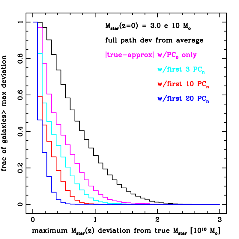
Figure 12: For the fiducial sample, the distribution of the maximum deviation of all galaxies from their true history (at any one given time $t_{i}$) from several different approximations: using the average of all galaxies (black histogram), only $PC_{0}$ (magenta histogram), and the first 3, 10, and 20 $PC_{n}$ (cyan, red, and blue histograms, respectively). Using a few $PC_{n}$ quickly brings many galaxy histories close to their true values.

In Fig. 12 we show the distribution of the largest deviation between true and approximate galaxy histories, at any one time $t_{i}$, for all of the galaxies in the fiducial sample. Five approximations are shown: $M_{\star}(t_{i})=$ the average history plus 0, first 1, first 3, first 10 or first 20 $PC_{n}$ contributions. Most of the histories become quite close to their true histories by the time 20 (less than half) of the $PC_{n}$ are used.

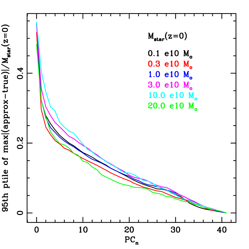
Figure 13: Approximating galaxy histories by a subset of $PC_{n}$: Statistics for all 6 Millennium samples: the 95th percentile of the maximum deviations at any given $t_{i}$ in a galaxy history, when keeping only the first $n$ $PC_{n}$. Fig.  12 gives an example of the distribution below the 95th percentile for going up to $PC_{0}$,$PC_{3},PC_{10}$ and $PC_{20}$ for the fiducial sample. The $y-axis$ value is rescaled by each sample’s final stellar mass to show general trends and allow more direct comparison.

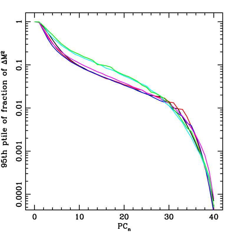
Figure 14: 95th percentile of fraction of the variance due to all $PC_{m}$ components, above $m\geq n$, i.e. keeping only up to and not including the $n$th $PC_{n}$ will omit this fraction of the variance or less for 95% of the galaxies, again for all Millennium samples. Colours as in Fig. 13 above.

To show trends with sample and with keeping increasing numbers of $PC_{n}$, the 95 percentile of maximum deviations ($|true-approximate|$ history at any given time) are shown in Fig. 13, for all 6 Millennium samples. The deviations are rescaled by the final stellar mass, to allow comparison between different samples and to highlight the similarities. The 95th percentile maximum deviation along a history can be large. However, the median largest deviation of each sample, for galaxy histories approximated at least up to $PC_{10}$, was at or below 16% of the 95% largest deviation. (Again, the shape of the distribution of large deviations for all galaxies is shown for the fiducial case in Fig. 12 above.) For $\Delta M^{2}$, approximately 10 $PC_{n}$ will get most galaxies in the four lower stellar mass samples within 10% of their true histories, a few more $PC_{n}$ are needed for the two highest final stellar mass samples. This can be seen in Fig. 14 bottom, showing the 95th percentile of the maximum $\Delta M^{2}$ difference between the true and approximate histories, when dropping a given $PC_{n}$ and above. This quantity pertains to the individual galaxy histories, although it is related to the total variance in the sample due to the respective principal components.

References

- Behroozi, Wechsler & Conroy (2013a) Behroozi, P.S., Wechsler, R.H., Conroy, C., 2103a, ApJ, 770, 57
- Behroozi, Wechsler & Conroy (2013b) Behroozi, P.S., Wechsler, R.H., Conroy, C., 2103b, ApJL, 762, 31
- Birrer et al. (2014) Birrer, S., Lilly, S., Amara, A., Paranjape, A., Refregier, A., 2014, arXiv:1401.3162
- Booth and Schaye (2009) Booth, C. M., Schaye, J., 2009, MNRAS, 398, 53
- Bryan et al. (2012) Bryan, S.E., Mao, S., Kay, S.T., Schaye, J., Dalla Vecchia, C., Booth, C.M., 2012, MNRAS,422, 1863
- Budavari et al. (2009) Budavari T., Wild V., Szalay A. S., Dobos L., Yip C.-W., 2009, MNRAS, 394, 1496
- Chen et al. (2012) Chen, Y.-M., et al, 2012, MNRAS, 421, 314
- Conroy, Wechsler & Kravtsov (2006) Conroy, C., Wechsler, R., Kravtsov, A.R., 2006, ApJ, 647, 201
- Conroy & Wechsler (2009) Conroy, C., Wechsler, R.H., 2009, ApJ, 696, 620
- Conti, Ryden and Weinberg (2001) Conti, A., Ryden, B.S., Weinberg, D.H., 2001, arXiv:astro-ph/0111001
- Dalla Vecchia and Schaye (2008) Dalla Vecchia, C., Schaye, J., 2008, MNRAS, 387, 1431
- Dolag et al. (2009) Dolag K., Borgani S., Murante G., Springel V., 2009, MNRAS, 399, 497
- Guo et al. (2013) Guo, Q., White, S., Angulo, R. E., Henriques, B., Lemson, G., Boylan-Kolchin, M., Thomas, P., Short, C., 2013, MNRAS 428, 1351
- Haas et al. (2013a) Haas, M.R., Schaye, J., Booth, C.M., Dalla Vecchia, C., Springel, V., Theuns, T., Wiersma, R.P.C., 2013, MNRAS, 435, 2955
- Haas et al. (2013b) Haas, M.R., Schaye, J., Booth, C.M., Dalla Vecchia, C., Springel, V., Theuns, T., Wiersma, R.P.C., 2013, MNRAS,435,2931
- Hearin & Watson (2013) Hearin, A.P., Watson, D.F., 2013, MNRAS, 435, 1313
- Hearin et al. (2013b) Hearin, A.P., Watson, D.F., Becker, M.R., Reyes, R., Berlind, A.A., Zentner, A.R., 2013, arxiv:1310.6747
- Hudson et al. (2013) Hudson, M.J., et al., 2013, arXiv1310.6784
- Jeeson-Daniel et al. (2011) Jeeson-Daniel, A., Dalla Vecchia, C., Haas, M.R., Schaye, J., 2011, MNRAS Letters, 415, 69
- Jolliffe (2002) Jolliffe, I.T., 1986, Principal Component Analysis. Springer Series in Statistics, Springer, Berlin
- Karim et al. (2011) Karim, A., et al, 2011, ApJ, 730, 61
- Leauthaud et al. (2011) Leauthaud, A., Tinker, J., Behroozi, P.S., Busha, M.T., Wechsler, R.H., 2011, ApJ, 738, 45
- Leitner (2012) Leitner, S., 2012, ApJ, 745,149
- Lemson et al. (2006) Lemson, G. & the Virgo Consortium, 2006, arXiv:astro-ph/0608019
- Lu et al. (2006) Lu, H., Zhou, H., Wang, J., Wang, T., Dong, X, Zhuang, Z., Li, C., 2006, AJ, 131, 790
- Lu et al. (2014) Lu, Z., Mo, H.J., Lu, Y., Katz, N., Weinberg, M.D., van den Bosch, F.C., Yang, X., 2014, MNRAS, 439, 1294
- Madau & Dickinson (2014) Madau, P., Dickinson, M., 2014, ARAA 52, to appear (arxiv:1403.0007)
- Madgwick et al. (2002) Madgwick, D.S., et al, 2002, MNRAS, 333, 133
- Mitchell et al. (2014) Mitchell, P.D., Lacey, C.G., Cole, S., Baugh, C.M., 2014, arxiv:1403.1585
- More et al. (2009) More, S., van den Bosch, F.C., Cacciato, M., Mo, H.J., Yang, X., Li, R., 2009, MNRAS, 392,801
- Moster et al. (2010) Moster, B.P., Somerville, R.S., Maulbetsch, C., van den Bosch, F.C., Maccio, A.V., Naab, T., Oser, L., 2010, ApJ, 710, 903
- Moster, Naab & White (2013) Moster, B.P., Naab, T., White, S.D.M., 2013, MNRAS, 428, 3121
- Mutch, Croton & Poole (2013) Mutch, S.J., Croton, D.J., Poole, G.B., 2013, MNRAS, 435, 2445
- Noh & Cohn (2012) Noh, Y., Cohn, J.D., 2012, MNRAS, 426,1829
- Oliver et al. (2010) Oliver, S., et al., 2010, MNRAS, 405, 2279
- Reddick et al. (2013) Reddick, R.M., Wechsler, R.H., Tinkder, J.S., Behroozi, P.S., 2013, ApJ, 771, 30
- Sales et al. (2010) Sales, L.V., Navarro, J.F., Schaye, J., Dalla Vecchia, C., Springel, V., Booth, C.M., 2010, MNRAS, 409, 1541
- Schaye et al. (2010) Schaye, J., et al., 2010, MNRAS, 402, 1536
- Simha et al. (2014) Simha, V., Weinberg, D.H., Conroy, C., Dave, R., Fardal, M., Katz, N., Oppenheimer, B.D., 2014, arXiv:1404.0402
- Skibba & Maccio (2011) Skibba, R. A., Maccio, A.V., 2011, MNRAS, 416, 2388
- Springel at al. (2001) Springel, V., White, S. D. M., Tormen, G., Kauffman, G. 2001, MNRAS, 328, 726S
- Springel et al. (2005) Springel, V., et al, 2005, Nature, 435, 629
- Tinker et al. (2013) Tinker, J.L., Leauthaud, A.s., Bundy, K., George, M.R., Behroozi, P., Massey, R., Rhodes, J., Wechsler, R.H., 2013, ApJ, 778, 93
- Vale & Ostriker (2006) Vale, A., Ostriker, J.P., 2006, MNRAS, 371, 1173
- van Daalen et al. (2011) van Daalen, M.P., Schaye, J., Booth, C.M., Dalla Vecchia, C., 2011, MNRAS, 415, 3649
- van de Voort et al. (2011) van de Voort, F., Schaye, J., Booth, C.M., Haas, M.R., Dalla Vecchia, C., 2011, MNRAS, 414,2548
- van de Voort and Schaye (2012) van de Voort, F., Schaye, 2012, MNRAS, 423,2991
- Wang et al. (2013) Wang, L., et al, 2013, MNRAS, 431, 648
- Wechsler et al. (2002) Wechsler, R.H., Bullock, J.S., Primack, J.R., Kravtsov, A.V., Dekel, A., 2002, ApJ, 568, 52
- Weinmann et al. (2012) Weinmann, S.M., Pasquali, A., Oppenheimer, B.D., Finlator, K., Mendel, J.T., Crain, R.A., Maccio, A.V., 2012, MNRAS, 426, 2797
- White (2001) White, M., 2001, A&A, 367, 27
- Wong and Taylor (2011) Wong, A.W.C., Taylor, J.E., 2011, ApJ, 757, 102
- Yang, Mo and van den Bosch (2009) Yang, X., Mo, H.J., van den Bosch, F.C., 2009, ApJ, 693, 830
- Yang et al. (2012) Yang, X., Mo, H.J., van den Bosch, F.C., Zhang, Y., Han, J., 2012, ApJ, 752, 41
- Yip et al. (2004a) Yip, C.W., et al, 2004, AJ, 128, 585
- Yip et al. (2004b) Yip, C.W., et al, 2004, AJ, 128, 2603