Multi-Scale Jacobi Method for Anderson Localization
Abstract
A new KAM-style proof of Anderson localization is obtained. A sequence of local rotations is defined, such that off-diagonal matrix elements of the Hamiltonian are driven rapidly to zero. This leads to the first proof via multi-scale analysis of exponential decay of the eigenfunction correlator (this implies strong dynamical localization). The method has been used in recent work on many-body localization [26].
1 Introduction
This work presents a new proof of localization in the Anderson tight-binding model at large disorder. In the spirit of KAM, a sequence of local rotations is used to diagonalize the Hamiltonian. This contrasts with previous work, which has largely focused on proving properties of the resolvent. Here we work directly with the eigenfunctions. We prove exponential decay of the eigenfunction correlator . Then strong dynamical localization is an immediate consequence. This work was motivated by a desire to find a procedure that might generalize to many-body Hamiltonians. We have successfully applied these ideas to a proof of many-body localization for a one-dimensional spin chain, under a certain assumption on level statistics [26]. The key to success in the many-body context is exponential bounds on probabilities, for example the probability that is not exponentially small. Such bounds have been proven by working with fractional moments of the resolvent [1], but here we present the first proof using multi-scale analysis. We have avoided using resolvent methods in this work because they do not seem to generalize to many-body problems.
Consider the random Schrödinger operator on :
| (1.1) |
Working on a rectangular subset , the Hamiltonian is an operator on :
| (1.2) |
Here we use the distance for . The potentials are iid random variables with a fixed, continuous distribution having a bounded density with respect to Lebesgue measure:
| (1.3) |
with
| (1.4) |
We prove exponential decay of the eigenfunction correlator for small , with bounds uniform in .
Theorem 1.1.
The eigenvalues of are nondegenerate, with probability 1. Let denote the associated eigenvectors. There is a such that if is sufficiently small (depending only on and ), the following bounds hold for any rectangle . The eigenfunction correlator satisfies
| (1.5) |
and consequently,
| (1.6) |
Dynamical localization refers to the rapid fall-off of with , where is the projection onto some energy interval . In the strong form, one has rapid decay of . Previous work has followed one of two paths. The multi-scale analysis program began with proof of absence of diffusion via analysis of resonant regions and associated bounds on the resolvent [20]. Subsequent work established dynamical localization in various forms by relating properties of the resolvent to properties of the eigenfunctions [28, 21, 13]. The best result was of the form for [22]. The dominant contribution to these bounds comes from probabilities of resonant regions. The fractional moment method began with a proof of exponential decay of for some [3]. Subsequent work used this result to obtain exponential decay of , thereby obtaining dynamical localization in the strongest form [1, 2, 25, 4].
Implicit in these results are bounds proving the rapid fall-off of the eigenfunction correlator , from which one obtains dynamical localization by bounding by 1. Chulaevsky has developed a hybrid approach [9, 10] with a greater focus on eigenfunction correlators.
In this work we focus on the unitary rotations that diagonalize the Hamiltonian. The columns of these rotations are the eigenfunctions. The rotation matrices are never singular, unlike the resolvent, which has poles at the eigenvalues. As a result, we are able to work with very mild separation conditions between resonant regions. This makes it possible to preserve exponential decay of probabilities of resonant regions. Exponential decay of probabilities is a critical requirement for progressing to many-body Hamiltonians, because the number of transitions possible in a region of size is exponential in .
We work on a sequence of length scales , designing rotations that connect sites separated by distances of the order of . In nonresonant regions, the rotations are written as convergent power series based on first-order perturbation theory. In resonant regions (blocks for quasi-degenerate perturbation theory), exact rotations are used, as in Jacobi diagonalization [31]. The procedure leads to rapid convergence to a diagonal Hamiltonian, with off-diagonal matrix elements . As the unperturbed eigenstates are deformed into the exact ones, we obtain a one-to-one mapping of eigenstates to sites (except in rare resonant regions, where states map to sites). The end result is a set of convergent graphical expansions for the eigenvalues and eigenfunctions, with each graph depending on the potential only in a neighborhood of its support. The detailed, local control of eigenvalues and eigenfunctions allows us to prove convergence in the limit. The expansions should be useful for a more detailed analysis of their behavior in both energy space and position space.
Previous authors have used KAM-type procedures in the context of quasiperiodic and deterministic potentials [6, 5, 30, 12, 11, 17, 18]. Other diagonalizing flows have been discussed in a variety of contexts [16, 7, 24, 32], but perhaps the closest connection to the present work is the similarity renormalization group [23].
2 First Step
In the first step, we derive an equation for the eigenfunctions of . At this stage, the expansion is just first-order perturbation theory in . In terms of the eigenfunctions , the state connects to nearest-neighbor states with . Multistep graphs will result when we orthonormalize the new basis vectors.
2.1 Resonant Blocks
We say that a pair sites and are resonant in step 1 if and . Take with . Let
| (2.1) |
This set can be decomposed into connected components or blocks based on the graph of resonant links . Each block is treated as a model space in quasi-degenerate perturbation theory, so we do not perturb with respect to couplings within a block. Our goal for this step is to find a basis in which is block diagonal up to terms of order .
Let us estimate the probability of , the event that two sites lie in the same resonant block. If occurs, then there must be a self-avoiding walk of resonant links from to . We claim that
| (2.2) |
Because is loop-free, we can change variables replacing with and the Jacobian is . Hence the probability that all the links of are resonant is less than , where is the number of links in .
2.2 Effective Hamiltonian
Having identified the resonant blocks and having estimated their probabilities, we proceed to perturb in the nonresonant couplings. Using the notation , write as a sum of diagonal and off-diagonal parts: with
| (2.3) |
| (2.4) |
Let us write
| (2.5) |
where only contains perturbative links with both endpoints outside . Links with at least one of in are in (could be resonant).
First-order Rayleigh-Schrödinger perturbation theory would give
| (2.6) |
Let us define an antisymmetric operator with matrix elements
| (2.7) |
Then, instead of (2.6), we use the orthogonal matrix for our basis change:
| (2.8) |
with taking the place of , which appears in (2.6). More generally, if were self-adjoint rather than symmetric, then would be unitary. A similar construction was used in [14, 15].
Let us write in the new basis:
| (2.9) |
Then we can define through
| (2.10) |
The matrix is no longer strictly off-diagonal. However, we will see that is of order , which is natural since energies vary only at the second order of perturbation theory when the perturbation is off-diagonal. In later stages we will need to adjust , but here we may use . Observe that :
| (2.11) |
Then, using , we have , and so
| (2.12) |
Here .
Observe that in the new Hamiltonian, and are still present, but is gone. In its place is a series of terms of the form or , with . Since , all such terms are of order with . This means that the new is of order . In particular, the matrix elements of satisfy
| (2.13) |
As in Newton’s method, the expansion parameter in each step will be roughly the square of the previous one.
We would like to interpret the above expressions for and in terms of graphical expansions. The matrix products or have a natural interpretation in terms of a sum of walks from to . At this stage, and allow only nearest neighbor steps. Thus we may write
| (2.14) |
where is a walk with nearest-neighbor steps, and
| (2.15) |
In view of the antisymmetry of , the links are oriented, and the walk runs from to . The graphical amplitude obeys a bound
| (2.16) |
where denotes the number of steps in .
In a similar fashion, we may write
| (2.17) |
A graph of consists of -links, followed by one link or , followed by -links, with . Thus specifies the following data: a spatial graph, , of unit steps in the lattice, and an assignment of or to one of the steps, with the rest being A-links. If we consider the set of denominators associated with the factors , we obtain a denominator graph, . The amplitude corresponding to is the product of the specified matrix elements and an overall factor easily derived from (2.12). For example, there is a term
| (2.18) |
(The binomial coefficient arises from expanding out and gathering like terms.) Since the prefactor is bounded by 1, we have an estimate:
| (2.19) |
Note that while is not symmetric under , the sum over consistent with a given spatial graph is symmetric (because is antisymmetric and is symmetric).
2.3 Small Block Diagonalization
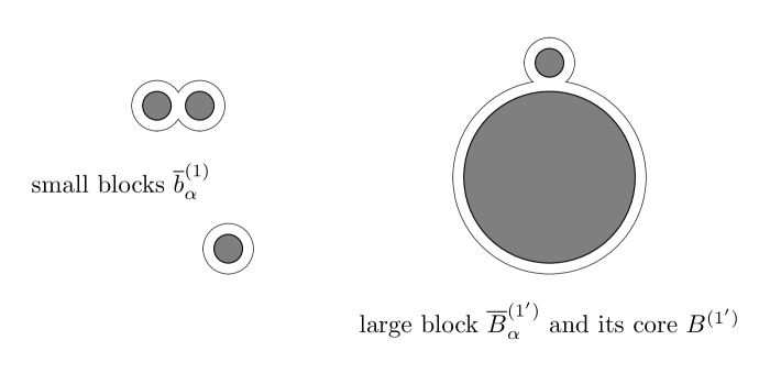
We have treated the nonresonant links perturbatively so as to diagonalize the Hamiltonian up to terms of order . In order to finish the first step we get rid of as many of the remaining terms as possible by diagonalizing within small blocks. Since there remains terms connecting the resonant region to its complement, we let be a thickened versions of , obtained by adding all first neighbors of . Then any term in the Hamiltonian with at least one end point in is necessarily second-order or higher. Components of with volume no greater than will be considered “small” (we take ). For such components, a volume factor will be harmless in the second step expansion, which has couplings . The volume factor arises from the sum over states in a block. Small components of will be denoted .
The remaining large components of will be denoted , and their union will be denoted . If we remove the one-step collar in each , we obtain . Likewise, . In this way we may keep track of the “core” resonant set that produced each large block .
It is useful to gather terms that are internal to the collared blocks and . The sum of such terms will be denoted ; the sum of the remaining terms will be denoted . Thus we write
| (2.20) | ||||
where contains terms of whose graph intersects a small block , and contains terms whose graph intersects a large block . These terms connect a block or to its collar. Then we have
| (2.21) |
We now diagonalize within small blocks . While we can find an orthogonal matrix that accomplishes this, we lose control over decay of eigenfunctions in the block. Let diagonalize . Note that the discriminant of the matrix is analytic in , so it cannot vanish on a set of positive measure without being identically zero. When the ’s are separated from each other by , it is clear that the eigenvalues are nondegenerate, and so the discriminant is nonzero. Thus the eigenvalues are nondegenerate and the rotation uniquely determined, with probability one. Note that each block rotation depends only on within the block. Since is block diagonal, is also. Let us define
| (2.22) |
where
| (2.23) |
is diagonal, and
| (2.24) |
Note that the rotation does not affect . Although first-order terms remain in , large blocks have many resonances and so can be considered high order after taking the expectation.
Observe from (2.17) that only has nonzero matrix elements between and , where is a walk from to . The rotation matrices extend the range of interaction for to the blocks containing and . Let label the set of terms obtained from the matrix product in (2.24); it adds at the start and finish of intra-block jumps associated with matrix elements of or . Thus includes these jumps as additional data; it represents a generalized walk whose first and last steps represent matrix elements of . Then we may write
| (2.25) |
Since the matrix elements of are bounded by 1, (2.19) leads immediately to the bound
| (2.26) |
where , the length of the walk ignoring intra-block jumps.
Although the eigenfunctions fail to decay in resonant blocks, if we integrate over we obtain exponential decay from the probabilities of blocks.
Proposition 2.1.
Let be sufficiently small. Then
| (2.27) |
We may think of the rows of as the eigenfunctions approximated to first order, and now including the effects of small blocks. This is another step towards proving (1.6).
Proof. Our constructions depend on the collection of resonant blocks, so (2.27) is best understood by inserting a partition of unity that specifies the blocks. Schematically, we may write
| (2.28) |
Here we sum over all possible collections of resonant blocks . The graphical expansion (2.15) for has to avoid resonant blocks. We insert it into (2.28) to obtain
| (2.29) |
We bound using (2.15). We may also bound by 1 since is an orthogonal matrix. Furthermore, if , and do not belong to the same block, the sum is zero because the rotations in distinct blocks have non-overlapping supports. In order for to be nonzero, must be both in the block of and in the block of . Thus, in place of we may insert an indicator for the event that and belong to the same small block . Then (2.29) becomes
| (2.30) |
where we have interchanged the sum over with the sum over , and used the fact that the sum of over compatible with is bounded by 1.
As in (2.2), the expectation on the right can be bounded by a sum of walks from to , with resonant conditions on the links. We have to allow for the one-step collar in , with nonresonant links. Still, there must be a (possibly branching) walk from to with at least of the steps resonant. Thus, we have a probability factor for each step of and a factor for each step of and . The number of branching walks of size is bounded by , where is a constant depending only on the dimension . After summing over and over the choice of factors or for each step of the walk, we obtain (2.27). ∎
3 The Second Step
3.1 Resonant Blocks
There are some issues that appear for the first time in the second step. Therefore, it is helpful to discuss them in the simplest case before proceeding to the general step.
In constructing resonant blocks , we will be allowing links of length 2 or 3 in the perturbation, which means that it is necessary to check for resonances between states up to 3 steps apart. Also, we must consider resonances between states in different blocks and between block states and individual sites.
Notation and terminology. Due to the fact that a block state is potentially spread throughout its block, we should consider a block as a “supersite” with multiple states. The rotation matrix has one site index and one state index, see for example (2.25). But it would be too cumbersome to maintain a notational distinction, so we will use to denote both sites and states. If a lattice point lies within a block, then the index may refer to one of the states in . The labeling of states within a block is arbitrary, so we may choose a one-to-one correspondence between the sites of and the states of , and use that to assign labels to states. Block states have many neighbors. We let denote the block of . This means that if is a site; otherwise is the block that gave rise to the state .
For each corresponding to a term of with , , , let us define
| (3.1) |
Here denotes a diagonal entry of . We call these terms “provisional” terms because not all of them will be small enough to include in . We only consider couplings between blocks or sites, never within a block or between a site and itself. Furthermore, only terms up to third order are considered in this step.
We say that from to is resonant in step 2 if is 2 or 3, and if either of the following conditions hold:
| (3.2) | ||||
Here is the distance from to in the metric where blocks are contracted to points. Condition II graphs are nearly self-avoiding, which allows for good Markov inequality estimates. Graphs with do not reach as far, so less decay is needed, and we can rely more on inductive estimates.
The graphs that contribute to have the structure , , , , where are one-step links from the first step. (Only terms contribute, because is gone and terms connect to some .) For example, if specifies an graph between sites , then
| (3.3) |
More generally, if either or is a block state, then the rotation matrix elements must be inserted as per (2.25). The resonance condition amounts to a condition on products of 2 or 3 energy denominations – one is , and the others are specified by .
We have to consider double- and triple-denominator resonant conditions because if, say, one had and , then the product would be . This is insufficient if one seeks a procedure which can be extended to all length scales. A complication with our definition of resonant events is their degree of correlation. In the first step, the correlation was mild because probabilities could be estimated in terms of uncorrelated Lebesgue integrals. In the present case, we use a Markov inequality argument to estimate each probability by a product of certain Lebesgue integrals. Still, if a graph has returns (loops) or if two graphs overlap at more than one vertex, then the probability estimate weakens due to correlations. This makes it harder to control event sums.
As mentioned above, overlapping graphs are problematic for our estimates. Therefore, we need to show that there is a sufficient number of non-overlapping graphs to obtain the needed decay in probabilities. The following construction generalizes to the step, so one may imagine the graphs being arbitrarily long.
Let us define the step 2 resonant blocks. Consider the collection of all step 2 resonant graphs . Two resonant graphs are considered to be connected if they have any sites or blocks in common. Then the set of sites/blocks that belong to resonant graphs are decomposed into connected components. The result is defined to be the step 2 resonant blocks . These blocks do not touch large blocks because resonant do not.
Note that all sites (states) within a small block are considered to be at a distance from each other, hence are automatically connected. In principle, one could explore connections between states of a block, but it is impractical because we only know how to vary block energies as a group; we have no control over intra-block resonances. Small blocks may be extended or linked together, and there may be entirely new blocks. Unlinked small blocks are not held over as scale 2 blocks.
Next we add a 3-step collar to all blocks as well as our leftover large blocks . This represents the range of sites reachable by graphs of the order considered in this step. Since steps may link to small blocks , the collar may extend farther than 3 lattice steps, depending on the configuration of small blocks. We do not expand links involving blocks at this stage, so the blocks need to expand into the region they could have linked to. As in the previous step, we define the resonant region to be the union of the blocks and . Then is the collared version of , and its components may be divided in to small blocks (volume ) and large blocks (volume ). The union of the is denoted , and then and .
We have constructed resonant blocks as connected components of a generalized percolation problem. The following proposition establishes exponential decay of the corresponding connectivity function.
Proposition 3.1.
Let denote the probability that lie in the same block or , and let be sufficiently small. Then
| (3.4) |
Proof. In the first-step analysis, there had to be an unbroken chain of resonant links from to . Here, we need to consider chains formed by and by resonant graphs , each thickened by three steps. (Let denote the thickened version of .) But when two graphs overlap, we cannot take the product of their probabilities. Correlation is manifested by the lack of independent variables with which to integrate the energy denominators. To overcome this problem, we find a collection of non-overlapping which extend at least half the distance from to . In this fashion, we may work with effectively independent events, while giving up half the decay.
Let be the resonant block containing . Define a metric on by letting be the smallest number of resonant graphs or blocks needed to form an unbroken chain from to . If , then there is a sequence of sites such that for , with each pair contained in some resonant graph or block. Note that the odd-numbered graphs/blocks form a non-overlapping collection of graphs; likewise the even-numbered ones. See Figure 3. For if the graph/block overlaps with the one with , then one could get from to in fewer than steps. This construction allows us to bound the probability of the whole collection of graphs/blocks by the geometric mean of the probabilities of the even and odd subsequences. Thus, we may restrict attention to non-overlapping collections of resonant graphs, losing no more than half the decay distance (from the square root in the geometric mean).

We have already proven that the probability that belong to the same block is bounded by – see the proof of Proposition 2.1. Let us focus, then, on a thickened resonant graph , and prove an analogous estimate.
Take the simplest case, , condition II of (3.2), with given by (3.3). Then by the Markov inequality, we have
| (3.5) |
for some fixed , say . Here is a bound for . This step involves a simple change of variable from the ’s to differences of ’s. By construction, the three sites/blocks are distinct, so the differences are independent. If or is in a block, we make a change of variables to difference variables on a tree spanning each block . But there is necessarily one variable left over corresponding to uniform shifts of the potential on that block. The energies come from diagonalizing on blocks. They move in sync with the variables for block shifts of the potential, since each block variable multiplies the identity operator on its block. Thus we can use and as integration variables, and the Jacobian is 1.
If , then an analogous bound
| (3.6) |
holds, provided is “self-avoiding,” i.e. it has no returns to sites or blocks, which would lead to fewer than three independent integration variables. If does have a return, then we have only condition I to worry about, because . The probability for condition I is easily seen to be , based on the size of the integration range. If we consider the bound on when , it is , because one denominator is and the other is . This will be adequate since we only need decay from to .
Let us now consider the bound on . In order for to occur, there must be a (possibly branching) walk from to consisting of
-
1.
at most 3 steps at the start and finish of large blocks and graphs . These steps have no small factor because of the collars employed in the construction of and .
- 2.
-
3.
Steps in lattice which are internal to large blocks or to a that is part of a resonant graph . These result in a small probability factor . Here we begin with , which is the probability of a resonant link at level 1, and add the exponent for the 1-step collar which may be present about any such link.
Note that in applying (3.5), (3.6), we are constrained to consider only the even- or odd-numbered graphs , because of the potential for shared or looping link variables. But all of the type (3) steps can be used because they involve difference variables within each . The Markov inequality bounds (3.5), (3.6) involve differences between block/site variables, so there is no overlap with the intra-block variables.
For each graph , there is a minimum of two type 2 steps and a maximum of 6 type 1 steps, see Figure 4. Therefore, each small factor from a type 2 step will be spread out over 4 steps by applying an exponent . Then every step has a factor no worse than . Each large block has volume greater than , which implies a diameter greater than . If we take , the diameter is at least 24. Adding 4 type 1 steps to allow for the collar increase from 1 to 3 on each side, we find that the linear density of resonant links may decrease from to .
Combining these facts, we may control the sum over (branching) lattice walks from to and over collections of resonant graphs along the walk as in the proof of Proposition 2.1. We obtain
| (3.7) |
which completes the proof of Proposition 3.1.
Remark. The sum over containing a particular point is straightforward at this stage, since it contains no more than 3 steps, and the number of states in a block is bounded by . We will need to be more careful when we revisit this estimate in the step.

3.2 Perturbation in the Nonresonant Couplings
Let us begin by making a split analogous to (2.5):
| (3.8) |
Here the perturbation terms are given by
| (3.9) |
and the “resonant” part consists of all terms with , terms intersecting , and diagonal/intrablock terms for which (the block of ) is the same as . Let us put
| (3.10) |
We would like to “resum” all terms from long graphs from to , i.e. those with . These are small enough, uniformly in , so there is no need to keep track of individual graphs and their -dependence. Let denote either a short graph from to or a special jump step from to whose length is defined to be . The jump step represents the collection of all long graphs from to . We call short or long accordingly. Then put
| (3.11) |
Now define the basis-change operator
| (3.12) |
and the new Hamiltonian
| (3.13) |
Recall that with . As in (2.12), we have
| (3.14) |
Note that since is second order in , all commutator terms are fourth-order or higher.
Let us describe the graphical expansions for and . As in (2.14), we may write
| (3.15) |
where is a walk consisting of a sequence of subgraphs . Then
| (3.16) |
Note that if we put together all the subgraphs of , we get a walk from to consisting of unit steps of short graphs and jump steps from long , in both cases between sites or blocks . In addition, there are jump steps within blocks from rotation matrix elements. The length is the sum of the constituent lengths – and as explained after (2.26), these do not include the intra-block jumps since there is no decay within blocks. Define the length of the spatial graph as the sum of the constituent lengths ignoring long graphs . The graph also determines a graph of energy denominators. Each short has one or two factors (each with an energy denominator with an cutoff) and an overall energy denominator with cutoff . The number of denominators always equals the number of steps because each is always short one denominator. Hence . (Long graphs are ignored on both sides of this equality.)
Nonresonant conditions (3.2) apply for links, so each in (3.16) is bounded by . As explained after (3.6), the bound for a long is . Allowing a constant for the number of long graphs from to , we find that for long . Hence
| (3.17) |
We continue with a graphical representation for , derived from (3.14):
| (3.18) |
Here is a generalized walk from to with a structure similar to that of . It consists of -links, followed by one -link or ), followed by -links, with . As above, -links are short or long (resummed) and indexed by ; -links are unchanged, indexed by . Note that in the case of , the subgraph can have length . Thus has an expression of the form (in the case of )
| (3.19) |
As in the case of , the spatial graph formed by uniting all the subgraphs forms a walk of unit steps and jump steps between blocks/sites, and jump steps within blocks. The denominator graph is short one link, compared with the non-jump steps of . Note that since and are both second-order or higher, all terms are of degree at least 4. If we apply nonresonant conditions (3.2) to and previous bounds (2.26) on , we see that
| (3.20) |
3.3 Small Block Diagonalization
In the last section we divided the current singular region into large blocks and small blocks with volume bounded by . By construction, any term of the Hamiltonian whose graph does not intersect is fourth-order or higher. Put
| (3.21) |
Here contains terms whose graph intersects and is contained in . Let include terms of that are contained in large blocks . Let include terms of that are contained in small blocks , as well as second- or third-order diagonal/intrablock terms for sites/blocks in . All remaining terms of and are included in . (There are some terms fourth-order or higher in that are now in – these were not expanded in (3.8)-(3.14) since they were already of sufficiently high order, and had too great a range.)
Let be the matrix that diagonalizes . It acts nontrivially only within small blocks. This includes blocks , which need to be “rediagonalized” due to the presence of intrablock interactions of second and third order. Then put
| (3.22) |
where
| (3.23) |
is diagonal, and
| (3.24) |
Note that is not affected by the rotation.
Recall the graphical expansions (3.18), (2.25), which define the terms from that contribute to . These are combined and rotated to produce an analogous graphical expansion for :
| (3.25) |
where specifies , a rotation matrix element , followed by a graph or , and then another rotation matrix element .
We complete the analysis of the second step by proving an exponential localization estimate for the rotations so far. Let us introduce cumulative rotation matrices:
| (3.26) | ||||
Proposition 3.2.
Let be sufficiently small. Then
| (3.27) |
Proof. Let us write
| (3.28) |
introducing as before a partition of unity for collections of blocks, and graphical expansions for each or matrix. The graphs combine to form a walk from to , with possible intra-block jumps.
We need to review how the rotations and fit together. By construction, is the identity plus a sum of terms involving products of , along with energy denominators – c.f. (2.26), (3.10), (3.16). Thus every matrix element is followed by a matrix element – except for the last one, which is followed by an matrix element. This structure follows naturally from the process of sequential basis changes. We need to distinguish between the identity matrix term in and the nontrivial terms. If we have the identity matrix, then we may form the matrix product before taking absolute values; then we may bound by 1 as before. For the nontrivial terms, the sum over states in the blocks as well as the sum over their sites are compensated by the smallness of , which must be present in this case. (We could also have taken advantage of the inequality at the intermediate blocks ; either way those sums are under control.) In step 2, the size of blocks is limited, so the state sums are of little consequence. But in the step we need to ensure that all state/site sums at blocks match up with appropriately small factors.
In all cases, intrablock jumps between two sites , are controlled by the probability that , belong to the same block or . Each of these probabilities has been estimated already in terms of a sum over walks from to with their associated small probability factors, c.f. the proofs of (2.2), (3.7). Therefore, we can bound (3.28) in terms of a sum over walks from to with at least a factor of per step. The bound (3.27) then follows. ∎
Remark. The decay in the nonresonant region is faster, with a rate constant , but in this integrated bound, we have to use the larger rate constant associated with resonant regions.
4 The General Step
Let us consider the step of the procedure, focusing on uniformity in . We work on a length scale , which is slightly smaller than the naïve scaling of Newton’s method. When long graphs are resummed, they are “contracted” to of their original length, and this reduces the length scale that can be treated in the following steps.
4.1 Starting Point
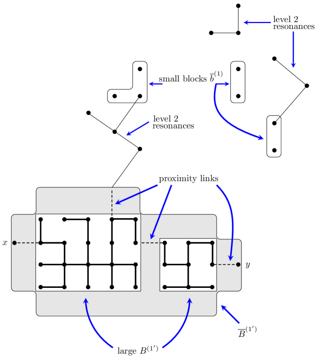
After steps, the structure of the resonant regions extends the picture in Figure 1. Small blocks have size up to , which is manageable because couplings in are at least at the conclusion of the step. Rotations have been performed in small blocks , diagonalizing the Hamiltonian there up to terms of order . Rotations are deferred for large blocks until is large enough for the volume conditions to be satisfied, at which point they may become small blocks. Collar neighborhoods of width are added to large blocks to form blocks . This is so that no couplings to are involved in the step expansion (the distance to is greater than , the maximum order for the step). In effect, the large blocks grow “hair” – unresolved interaction terms of length up to which could not be expanded because they are not small enough to beat the volume of the block. See Figure 5.

We maintain a uniform bound as in (3.7) on , the probability that belong to the same large block or small block .
Resonances treated in step involve graphs with , so the associated probabilities are of that order in . Nonresonant couplings in step are of the same order in . Couplings and resonance probabilities decrease in tandem as increases, a key feature of our procedure.
Let us recapitulate the transformations from the step. After defining resonant blocks , the Hamiltonian was rewritten as follows:
| (4.1) |
The terms in were “rotated away” by conjugating with . This led to a new Hamiltonian with smaller interactions and after regrouping terms, it became
| (4.2) |
Rotations were performed in small blocks, and low-order diagonal terms were absorbed into , leading to a form like the one we started with:
| (4.3) |
The rotation has a graphical expansion
| (4.4) |
as in (3.15), and as in (3.17) we have a uniform bound
| (4.5) |
This arises from the more basic estimate:
| (4.6) |
Here we define for any and any jump step from to :
| (4.7) |
Here is the distance from to in the metric where blocks on scales are contracted to points. Likewise, the interaction terms and have graphical expansions generalizing (3.25). Thus
| (4.8) |
with bounds as in (3.20):
| (4.9) |
The graphs and are actually “walks of walks,” with each step representing a walk from the previous scale. When unwrapped to the first scale, we obtain spatial graphs and , as well as denominator graphs and . Resummed sections appear as jump steps with no denominators. Likewise, rotation matrix elements appear as jump steps within blocks.
The goal of each step is to prove a bound analogous to (3.27):
| (4.10) |
where
| (4.11) |
is the cumulative rotation matrix, whose columns represent the eigenfunctions approximated up to scale .
4.2 Resonant Blocks
Here we make straightforward generalizations of definitions from step 2. Let be a graph that does not intersect any , with (recall that ). Define
| (4.12) |
where is the same as , except jump steps that are subgraphs of are replaced with their upper bound from (4.6). We say that from to is resonant in step if either of the following conditions hold:
| (4.13) | ||||
It may be helpful to explain the key ideas behind maintaining uniform exponential decay in our constructions. A resonant graph can be thought of as an event with a small probability. In order for a collection of graphs to be rare, we need to be able to sum the probabilities. In the ideal situation, where there are no repeated sites/blocks in the graph, the probability is exponentially small, so it can easily be summed. However, when graphs return to previously visited sites, dependence between denominators develops, and then the Markov inequality that is used to estimate probabilities begins to break down. Subgraphs in a neighborhood of sites with multiple visits need to be “erased,” meaning that inductive bounds are used, and they do not participate in the Markov inequality. (By this we mean that the bound is used when is bound for – so the variation of is not helping the bound.) When there are a lot of return visits, a graph’s length is shortened by at least a factor , and it goes into a jump step, where again we use inductive bounds. In this case, we have more factors of , and hence a more rapid decay, and this provides the needed boost to preserve the uniformity of decay in the induction. (Fractional moments of denominators are finite, no matter the scale, which provides uniformity for “straight” graphs with few returns.) The net result is uniform probability decay, provided we do not sum over unnecessary structure, i.e. the substructure of jump steps. Note that jump steps represent sums of long graphs, so when taking absolute values it is best to do it term by term. This is why we replaced jump steps with their upper bound in (4.12). (The jump step bound (4.6) is also a bound on the sum of the absolute values of the contributing graphs.)
Now consider the collection of all step resonant graphs . Any two such graphs are considered to be connected if they have any sites or blocks in common. Decompose the set of sites/blocks that belong to resonant graphs into connected components. The result is defined to be the set of step resonant blocks . By construction, these blocks do not touch large blocks . Small blocks can become absorbed into blocks , but only if they are part of a resonant graph .
A collar of width must be added to all blocks and because we will not be expanding graphs of that length that touch any of those blocks. Let be the union of the blocks and . Then is the collared version of , and its components are divided into small blocks (volume and large blocks (volume . The union of the is denoted , and then and .
As discussed in Section 3.1, if belong to the same resonant block , then there must be a sequence of resonant graphs connecting to with the property that the even and odd subsequences consist of non-overlapping graphs. This allows us to focus on estimating probabilities associated with individual resonant graphs.
The next three subsections establish key results that will be needed in the proof of Proposition 4.1, the main “percolation” estimate that is the core of our method. The final subsection will complete the proof, thereby establishing exponential decay of the probability that , lie in the same resonant block.
4.2.1 Graphical Sums
Before getting into a discussion of resonance probabilities, we need to understand more about how to sum over multi-scale graphs . The goal is to replace any sum of graphs with a corresponding supremum, multiplied by a factor . Graphical sums occur both in the ad expansion for the effective Hamiltonian and in estimates for percolation probabilities.
If a graph executes an ordinary step in the lattice, a factor will account for the number of choices. If we have a jump step from to , a factor can be used – this overcounts the number of possibilities, but matches against the power of or that is available for bounds on resonance probabilities or perturbative expansion links. We also pick up factors of when the walk passes through a small block . These arise from the block rotation matrices, which lead to sums over states in blocks, as well as sums over lattice sites in blocks that may serve as starting points for walks proceeding onward. In effect, the coordination number of such vertices can be very large. But by construction, the minimum graph length for any step into a is . Of course, , but we need to be cognizant of the fact that in a multi-scale graph, we cannot get away with repeatedly introducing factors . But with the exponent, we see that the combinatoric factor per step from scale is actually . Then noting that , the sum of converges, and the overall combinatoric factor from blocks of all scales is bounded by .
There are other counting factors that need to be considered. For example, in each step the expansion of produces a sum of terms as in (2.18). We also need to sum on . There is also the choice of whether to take a jump step or a regular step as we need to consider both alternatives in (3.11). Overall, the number of choices is bounded by . Again, since the minimum graph length for a step on scale is , the overall combinatoric factor is . We can see the power of quadratic convergence (or in our case convergence with exponent ) in controlling combinatoric factors. If grew only linearly with , the combinatoric factors would grow without bound.
4.2.2 The Jacobian
Our method for estimating probabilities of resonant graphs involves a Markov inequality, taking an expectation of a graph to the power, and making a bound in terms of a product of one-dimensional integrals. In the first step, we could take the integration variables to be the energy denominators , as long as they form a tree graph. In the second step, some denominators involved block energies , but as these moved in sync with uniform shifts of in blocks, they could be used as independent integration variables as well. To continue this process we have to allow for energy corrections that were moved into from at the end of step . These terms are bounded like any other interaction terms as in (4.9) – they just happen to be diagonal. However, if energies are to be used as integration variables, we need to control the Jacobian for the change of variable. Energy correction terms for depend on energies for up to steps away (the graph has to loop back to and contain ). So we need to consider the product of Jacobians over . Here are restricted to the particular graph whose expectation we are trying to bound. As explained above in the case of block energies , all but one of the integration variables in a block can be replaced with energy differences, and the remaining variable can be shifted to the energy that appears in . The variable then represents constant shifts in energy throughout the block. In this way, all of the energy denominators in can be used as integration variables, with the Jacobian for each intra-block change of variable equal to 1. Everything is contingent on the denominator graph being loop free, with any returns to a block counted as a loop. We can, however, work on a loop-free subgraph of .
We now show how to bound . Here belong to the subgraph of corresponding to the level steps of . (Note that energy denominators produced in steps retain their step indices – see (3.3) for a simple example. Assume, for the moment, that are site variables, i.e. they do not belong to blocks. Energy correction terms in are bounded as in (4.9). When differentiated with respect to , each term is replaced with a sum of terms with one of the denominators containing being duplicated. The extra denominator can be bounded as in (4.13I). Thus the derivative can be bounded by , where the constant is inserted to account for the sum over the denominators containing . Summing over that go from to via , we obtain a bound
| (4.14) |
which applies as well to .
If block variables are involved, then there is a complication because the energies are determined through a two-step process. First, the graphical expansions determine a shift in the effective Hamiltonian of the block. Second, the energy shifts are determined by the change in the eigenvalues when the block is “rediagonalized.” But Weyl’s inequality implies that the eigenvalues are Lipschitz continuous in the matrix entries. The leading term in the map from the variables to the variables is the identity matrix. Hence the map is bi-Lipschitz, and by Rademacher’s theorem the Jacobian is well-defined almost everywhere, and the Lipschitz constant bounds the partial derivatives in the Jacobian matrix. The usual change of variable formula holds in this context [19]. Thus the argument above applies as well to the cases involving block variables. Intuitively, one needs control of the measure of regions determined by level surfaces of for the inverse map; Lipschitz continuity is sufficient for this.
Let us assume that the matrix indices run over a set of sites/states. Normally, these are the vertices of some graph , or a subgraph. From the discussion above on the combinatorics of graphical sums, we see that row and column sums of are bounded by , because . Note that all contribute here, not just subgraphs of . We conclude that all eigenvalues of are in a correspondingly small neighborhood of 1. Therefore,
| (4.15) |
Due to the rapid growth of , this can be summed on to give a bound on the product of all the Jacobian determinants incurred in using energy denominators as integration variables. This bound can easily be absorbed into probability estimates, which are exponentially small in .
4.2.3 Resonant Graphs
We are now ready to estimate probabilities of resonant graphs as in (3.5). First, let us consider a graph with no returns. Then the denominator graph likewise has no loops. (In the absence of jump steps it has the same number of links as the spatial graph, and the same vertices. See below for a general argument.) Then
| (4.16) |
Here is the denominator graph for , which is plus the denominator for . Note that the power of in equals , so the ’s factor out of (4.16). The second bound of (4.6) ensures that jump steps contribute their share of factors. After the change of variable discussed above, each is an independent variable. We integrate each link, and find that (4.16) is bounded by (we absorb factors of from the Jacobian into ). The probability for condition I of (4.13) can likewise be bounded by by a similar Markov inequality for the single denominator or more simply by noting the length of the integration domain where (4.13I) holds.
Now we need to consider the general case for (4.13II), with “nearly self-avoiding,” i.e. . Any return to a site or block will necessarily shorten the total distance , because of the “wasted” steps. We can make this quantitative by drawing a timeline for the walk (graph) , with ordinary steps counting as one time unit, and jump steps of length counting as time steps. Any time the walk returns to a site/block, we draw an “arch” connecting the return time to the time of the first visit. The arch graph breaks into connected components, with all sites/blocks on the graph between the components being visited exactly once. This is similar to the lace expansion for self-avoiding walks [8]. Each component represents a time interval during which the walk is executing loops.
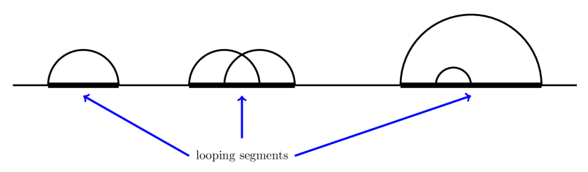
A simple loop/arch of length will cut back the distance traveled by . More generally, a looping segment of length will cut back the distance traveled by at least . This is because the spatial graph of the looping portion of the walk is triply connected. That is, any surface separating (the starting point of the looping section) from (the final point) will be crossed at least three times by the walk. (Topologically, the number of crossing must be odd, and a singlet crossing would disconnect the segment.) As a result, the length of the graph within the looping segment must be at least three times the distance from to , so of the steps are “wasted”. We can conclude that the sum of the lengths of the looping segments cannot be greater than .

The next step is to identify certain time intervals containing the looping segments where inductive bounds (non-probabilistic) will be used in place of Markov inequality bounds. We will need to keep a reasonable fraction of the timeline out of the covering intervals, otherwise we will not get the needed probability decay with . The denominator graph has long-range links, so looping segments will affect the character of the denominator graph in some neighborhood.
If we consider the denominator graph prior to the identification of vertices on the timeline, it is devoid of loops. This is because each time a denominator is produced, it connects one or more loop-free graphs to a disconnected, loop-free graph . (More precisely, for a graph of that goes from to , does not connect to , so the new denominator cannot create a loop.) Some denominators are dropped when they are incorporated into jump steps, but this does not spoil the loop-free property. (It is useful to keep in mind the “nested” character of the denominator links. Graphs are constructed as “walks of walks,” so the denominator in encompasses all the previous ones in on the timeline of .) Let be the looping segment of the timeline, and let be its length. Let and let be such that . Let us consider the denominator subgraph formed by the links introduced in step and afterwards, with timeline length in the range . As a subgraph of a loop-free graph, is of course loop free. Furthermore, even after the identification of sites within looping intervals, it remains loop-free. This is because each denominator connects sites at least apart on the timeline, while identifications only occur within disjoint intervals of length .
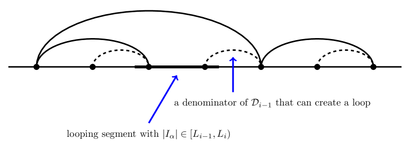
Next, consider what happens when we add denominators from the step, connecting points with timeline separations in . Some of these may be internal to one of the looping segments, and we will have to replace the corresponding ’s by uniform bounds from (4.6). The denominator is effectively erased from the denominator graph, along with all denominators nested inside. A denominator with only one endpoint in a segment is dangerous if because it could link back indirectly to another point in the segment through denominators on scales . Therefore, for such a denominator, we replace the corresponding by its bound . It is not necessary to erase denominators on both sides of , because can produce at most one identification of sites in the denominator graph at this stage. (The interval cannot contain more than two vertices of , because a third would force it to have length .) Hence the removal of one denominator link is sufficient to restore the loop-free property. Through this construction, we obtain a loop-free denominator graph , consisting of non-erased denominators on scales . We continue the process to smaller length scales , ,…, and the scale of the “erased” denominators never exceeds the scale of the looping segment it originates from. When the process concludes, we obtain a loop-free denominator graph . Each looping segment has a collar of erased sections of width on one side, and on the other, for . The looping interval “spoils” a neighborhood of size no larger than . The total length of the “spoiled” intervals where non-probabilistic bounds are employed is .
We return to the probability bound as in (4.16), only now we allow any graph with . We obtain
| (4.17) |
The “erased” sections of contribute factors of instead of in the expectation, so they contribute no smallness to the probability estimate. But at least of is clear of looping problems, and so we are able to glean factors of in the Markov inequality.
4.2.4 Block Probabilities.
The basic resonance probability bound (4.17) ensures a positive density of factors of on the walk from to used to estimate , the probability that , belong to the same resonant block or . Following the proof of the analogous bound (3.7) for , we pick up powers of as the walk traverses resonant blocks on different scales, and resonant graphs on the current scale. Each step of a resonant graph produces a factor from (4.17), but this becomes because of the square root in the non-overlapping graph construction. There is a further degradation of decay due to the scale collar, which has width . The minimum length of a resonant graph is , so the density of factors of is reduced by a factor , leaving a residual factor per link. This would be the uniform rate of probability decay, except for the fact that large resonant blocks from earlier scales have their collars increased to . The increase in the step is from to , for a total increase along the walk of . The diameter of the block is at least , so the density of factors of is reduced slightly by a factor of in the step. The rapid growth of with ensures that the density of factors of does not drop below . (We treated step 2 explicitly in step 2, and subsequent steps have a minor effect due to the large volumes involved.) After summing over the graphs in the walk from to with the combinatoric bounds established above, we obtain the following result:
Proposition 4.1.
Let be sufficiently small. Then
| (4.18) |
4.3 Perturbation Step and Proof of Inductive Bounds.
Let us repeat the analysis of Section 3.2, writing
| (4.19) | ||||
| (4.20) | ||||
| (4.21) |
As before, we resum all terms from long graphs with . Let denote either a short graph or a jump step representing all resummed terms. Then let
| (4.22) |
With , we obtain
| (4.23) |
We prove our inductive bounds (4.6, (4.9) for . For short graphs, we claim that
| (4.24) |
To see this, replace jump step subgraphs with their upper bounds from (4.6). This transforms into – see definition (4.12). Then is bounded because is nonresonant, c.f. condition (4.13II). For long graphs, we bound numerator and denominator separately in (4.21). The inductive bound (4.9) applies to the numerator, and the resonant condition (4.13I) bounds the denominator from below. As a result, we have
| (4.25) |
After summing over long graphs from to , we obtain
| (4.26) |
because all long graphs have , see (4.7). Recall that with . So , and we obtain
| (4.27) |
which completes the induction for . Note that this proof and bound applies also to the sum of the absolute values of long graphs. (Since (4.27) is a stronger estimate, we have for all .) Let us now examine , which involves terms with a and one or more factors. Combining (4.9) with the bounds just proven for , we obtain the estimate
| (4.28) |
which will lead to a proof of (4.9) for after the block rotations are performed. Note that by (4.7), the minimum size of in an term is . The minimum size of a graph is . Combining these, we obtain a minimum size of for graphs .
4.4 Diagonalization and Conclusion of Proof
As in Section 3.3, we reorganize terms, putting
| (4.29) |
Terms whose graph intersects and is contained in are put in (small block terms) or (large block terms). Diagonal/intrablock terms for sites/blocks in are included in if they are of order less than . This is so that in the next step, commutators will not produce terms whose order is less than what is required.
Let be the matrix that diagonalizes small blocks. Then
| (4.30) |
is the new diagonal part of the Hamiltonian. Then put
| (4.31) |
Here is the rotated version of ; it has a graphical expansion with bounds as in (4.8), (4.9).
Let us examine the cumulative rotation and prove the “eigenfunction correlator” estimate, as claimed in (4.10):
Proposition 4.2.
Let be sufficiently small. Then
| (4.32) |
Proof. We proceed as in the proof of Proposition 3.2. The graphical expansions for the matrices , , lead to walks that extend from to with decay constant . With a partition of unity argument as in (2.28)-(2.30), the gaps in this walk due to blocks can be filled in with “probability walks” along resonant graphs, as in the proof of Proposition 4.1. As discussed in the proof of Proposition 3.2, small block rotations are combined when not separated by perturbative graphs. The net result is a combination walk from to with a minimum density of factors of . All of the walks and state sums are under control, from the discussion on graphical sums in Subsection 4.2.1. ∎
Proof of Theorem 1.1. If we let the procedure run to , off-diagonal matrix elements vanish in the limit. Then the eigenvalues of the starting Hamiltonian are given by the diagonal elements of . They are almost surely nondegenerate, by the argument given in Section 2.3. Note that block formation has to stop eventually in a finite volume , and after that, the effective Hamiltonian converges rapidly with . Indeed, the off-diagonal entries of decay exponentially with . By Weyl’s inequality, changes in the diagonal entries of are correspondingly small. Hence they converge rapidly to the eigenvalues of , which are nondegenerate. Once the off-diagonal entries are much smaller than differences in the diagonal entries, the rotation matrices used in our procedure are correspondingly close to the identity. Hence we can define , and the eigenfunctions of are given by the columns of this limiting rotation. By bounded convergence, (4.32) remains true in the limit. This completes the proof of Theorem 1.1. ∎
One could improve considerably on the rate of decay proven here, but we have focused on constructing the simplest exposition of the method, rather than optimizing estimates.
4.5 Labeling of Eigenfunctions and Infinite Volume Limit
Each eigenstate has an abstract label . However, working pointwise in the probability space, one finds that outside of blocks, there is a one-to-one correspondence between states and sites of the lattice, because each eigenstate has an expansion exhibiting the predominance of amplitude at a particular site. In blocks, there are potentially some choices that need to be made in assigning labels to states. Labels are assigned when a diagonalization step is performed in a block. As explained earlier, the eigenvalues are nondegenerate, with probability 1. Therefore, except for a set of measure zero, one can label block states in order of increasing energy. The percolation estimate (4.18) establishes the diluteness of blocks, without which the labeling system would lose its significance. From the estimate (1.6) on the eigenfunction correlator, we see that eigenfunctions are exponentially small in the distance from the site that they are associated with, except for a set of exponentially small probability.
As discussed in Subsection 4.2.2, eigenvalues have been given convergent graphical expansions, with exponential decay in the size of the graph, c.f. (4.9). Eigenfunctions likewise have a local graphical expansions. Let us use these expansions to demonstrate almost sure convergence of eigenvalues and eigenfunctions as increases to . Let . When considering the limit, it is convenient to use a -independent definition of resonant blocks. In each step of our procedure, a graph will be considered resonant if it is resonant for any value of . Then, in addition to the usual graphical sums for estimating probabilities of resonances, there is a sum over values of that lead to distinct resonant conditions for a given graph. The sum over can be handled in the same manner as the volume factors already taken into account in our estimates (c.f. Subsection 4.2.1). (We need to sum over the different ways can intersect the graph and all the sites/blocks that affect it – even indirectly through graphical expansions of the energies of the graph.) Thus we maintain bounds as in (4.17) on the probabilities of these generalized resonant graphs.
With this modified procedure, we may work with a fixed configuration of resonant blocks for all values of . For each block , we choose a canonical method of associating sites of with the states of that block, for example by using lexicographic order on the sites of and matching them to states in order of increasing energy. We may consider, then, the question of convergence of the eigenvalues and eigenfunctions associated with a particular site .
Theorem 4.3.
Let be sufficiently small, and assume that the probability distribution of the potentials has bounded support. Let denote the eigenvalues and eigenfunctions of , labeled according to the system described above. Then and exponentially almost surely as , with the limits satisfying . Furthermore, converges exponentially almost surely as for each , , and the limit satisfies
| (4.33) |
for some chosen independently of .
Proof. Compare the graphical expansions of the eigenvalues associated with in two different boxes, and , with . The difference involves graphs that extend to . (Jump steps need to be rewritten as sums of constituent graphs so as to isolate the ones extending to .) Consider the event in which there exists a path from to with length less than dist, in the metric where blocks are contracted to points. By summing over paths and over configurations of blocks along each path, it should be clear that decays exponentially like for some . By Borel-Cantelli, there is almost surely a such that fails for all . Bounds on a given graph are governed by the distance it covers between blocks. Hence, as long as , we obtain bounds that decay exponentially in . This means that differences between effective Hamiltonians of the block from the change are exponentially small, once . By Weyl’s inequality, the same is true for the eigenvalues associated with , in particular for , the eigenvalue of that is associated with .
In order to get a similar statement for the corresponding eigenfunction , we need some quantitative control on the gaps between the eigenvalues associated with . For simplicity, we have assumed that the probability distribution of the potentials is supported on a bounded interval. Consider the spectrum of , which is then also supported on a bounded interval. Let be the event that there is a gap smaller than . From Minami’s estimate [29], one can show that is bounded by a constant times , for – see [27], eq. 8. Taking , the probabilities are summable, so by Borel-Cantelli there is almost surely a such that fails for all . As explained above, differences between corresponding effective Hamiltonians of the block from the change are exponentially small, so for they are much smaller than the gaps between eigenvalues associated with . (Here we use the fact that these eigenvalues agree with those of within an exponentially small error, as explained in the proof of Theorem 1.1.) This implies that the mixing of with the other eigenfunctions associated with are similarly small. Thus we obtain almost sure exponential convergence of both and as . Observe that as because only affects at the boundary of , and the relevant graphs are exponentially small in . Hence almost surely.
The same arguments can be used to demonstrate almost sure exponential convergence of as for each , , because the graphs involved extend from to . By bounded convergence, the eigenfunction correlator estimate of Theorem 1.1 extends to the limits , , completing the proof. ∎
Acknowledgement
The author would like to thank Tom Spencer for a collaboration over several years, during which time many of these ideas were developed. Comments from Wojciech De Roeck were helpful in improving an earlier draft of this work.
References
- [1] Aizenman, M. Localization at weak disorder: Some elementary bounds. Rev. Math. Phys. 06 (1994), 1163–1182.
- [2] Aizenman, M., and Graf, G. M. Localization bounds for an electron gas. J. Phys. A. Math. Gen. 31 (1998), 6783–6806.
- [3] Aizenman, M., and Molchanov, S. Localization at large disorder and at extreme energies: an elementary derivation. Commun. Math. Phys. 157 (1993), 245–278.
- [4] Aizenman, M., Schenker, J. H., Friedrich, R. M., and Hundertmark, D. Finite-volume fractional-moment criteria for Anderson localization. Commun. Math. Phys. 224 (2001), 219–253.
- [5] Bellissard, J., Lima, R., and Scoppola, E. Localization in -dimensional incommensurate structures. Commun. Math. Phys. 88 (1983), 465–477.
- [6] Bellissard, J., Lima, R., and Testard, D. A metal-insulator transition for the almost Mathieu model. Commun. Math. Phys. 88 (1983), 207–234.
- [7] Brockett, R. W. Dynamical systems that sort lists, diagonalize matrices, and solve linear programming problems. Linear Algebr. Appl. 146 (1991), 79–91.
- [8] Brydges, D., and Spencer, T. Self-avoiding walk in 5 or more dimensions. Commun. Math. Phys. 97 (1985), 125–148.
- [9] Chulaevsky, V. Direct scaling analysis of localization in single-particle quantum systems on graphs with diagonal disorder. Math. Physics, Anal. Geom. 15 (2012), 361–399.
- [10] Chulaevsky, V. From fixed-energy localization analysis to dynamical localization: An elementary path. J. Stat. Phys. 154 (2014), 1391–1429.
- [11] Chulaevsky, V., and Dinaburg, E. Methods of KAM-theory for long-range quasi-periodic operators on . Pure point spectrum. Commun. Math. Phys. 153 (1993), 559–577.
- [12] Chulaevsky, V., and Sinai, Y. The exponential localization and structure of the spectrum for 1D quasi-periodic discrete Schrödinger operators. Rev. Math. Phys. 03 (1991), 241–284.
- [13] Damanik, D., and Stollmann, P. Multi-scale analysis implies strong dynamical localization. Geom. Funct. Anal. 11 (2001), 11–29.
- [14] Datta, N., Fernández, R., and Fröhlich, J. Low-temperature phase diagrams of quantum lattice systems. I. Stability for quantum perturbations of classical systems with finitely-many ground states. J. Stat. Phys. 84 (1996), 455–534.
- [15] Datta, N., Fernández, R., and Fröhlich, J. Effective Hamiltonians and phase diagrams for tight-binding models. J. Stat. Phys. 96 (1999), 545–611.
- [16] Deift, P., Nanda, T., and Tomei, C. Ordinary differential equations and the symmetric eigenvalue problem. SIAM J. Numer. Anal. 20 (1983), 1–22.
- [17] Eliasson, L. Discrete one-dimensional quasi-periodic Schrödinger operators with pure point spectrum. Acta Math. 179 (1997), 153–196.
- [18] Eliasson, L. Perturbations of linear quasi-periodic system. In: Dynamical Systems and Small Divisors Springer, 2002, pp. 1–60.
- [19] Evans, L. C., and Gariepy, R. F. Measure theory and fine properties of functions. CRC Press, 1991.
- [20] Fröhlich, J., and Spencer, T. Absence of diffusion in the Anderson tight binding model for large disorder or low energy. Commun. Math. Phys. 88 (1983), 151–184.
- [21] Germinet, F., and De Bièvre, S. Dynamical localization for discrete and continuous random Schrödinger operators. Commun. Math. Phys. 194 (1998), 323–341.
- [22] Germinet, F., and Klein, A. Bootstrap multiscale analysis and localization in random media. Commun. Math. Phys. 222 (2001), 415–448.
- [23] Głazek, S., and Wilson, K. Renormalization of Hamiltonians. Phys. Rev. D 48 (1993), 5863–5872.
- [24] Grote, I., Körding, E., and Wegner, F. Stability analysis of the Hubbard model. J. Low Temp. Phys. 126 (2002), 1385–1409.
- [25] Hundertmark, D. On the time-dependent approach to Anderson localization. Math. Nachrichten 214 (2000), 25–38.
- [26] Imbrie, J. Z. On many-body localization for quantum spin chains. arXiv:1403.7837.
- [27] Klein, A., and Molchanov, S. Simplicity of eigenvalues in the Anderson model. J. Stat. Phys. 122 (2006), 95–99.
- [28] Martinelli, F., and Scoppola, E. Introduction to the mathematical theory of Anderson localization. La Riv. Del Nuovo Cim. 10 (1987), 1–90.
- [29] Minami, N. Local fluctuation of the spectrum of a multidimensional Anderson tight binding model. Commun. Math. Phys. 177 (1996), 709–725.
- [30] Sinai, Y. Anderson localization for one-dimensional difference Schrödinger operator with quasiperiodic potential. J. Stat. Phys. 46 (1987), 861–909.
- [31] Sleijpen, G., and Van der Vorst, H. A Jacobi-Davidson iteration method for linear eigenvalue problems. SIAM Rev. 42 (2000), 267–293.
- [32] Wegner, F. Flow equations and normal ordering: a survey. J. Phys. A. Math. Gen. 39 (2006), 8221–8230.