Theoretical analysis of the astrophysical S- factor for the $\alpha+d\rightarrow^{6}Li+\gamma$ capture reaction in the two body model

Abstract

Theoretical estimations for the astrophysical S-factor and the $d(\alpha,\gamma)^{6}Li$ reaction rates are obtained on the base of the two-body model with the $\alpha-d$ potential of a simple Gaussian form, which describes correctly the phase-shifts in the S-, P-, and D-waves, the binding energy and the asymptotic normalization constant in the final S-state. Wave functions of the bound and continuum states are calculated by using the Numerov algorithm of a high accuracy. A good convergence of the results for the E1- and E2- components of the transition is shown when increasing the upper limit of effective integrals up to 40 fm. The obtained results for the S-factor and reaction rates in the temperature interval $10^{6}K\leq T\leq 10^{10}K$ are in a good agreement with the results of Ref. A.M.  Mukhamedzhanov, et.al., Phys. Rev. C 83, 055805 (2011), where the authors used the known asymptotical form of wave function at low energies and a complicated potential at higher energies.

I Introduction

It is well known that the ⁶Li nuclei have been formed mainly as a result of the Bing Bang through the capture reaction

$$\alpha+d\rightarrow^{6}Li+\gamma$$ (1)

at low energies $50\leq E_{cm}\leq 400$ keV ser04 . This process was studied in details by the experimental groups at energies around the $3^{+}$ resonance with $E_{cm}=$0.711 MeV and at higher energies mohr94 ; robe81 . However, at low energies the obtaining an information on the cross section of the process from the analysis of the experimental data met insuperable difficulties kien91 ; hamm10 . In the recent work hamm10 the break up process of the ${}^{6}Li$ nucleus in the field of heavy ion ${}^{208}Pb$ was studied with the aim to extract data on the cross section of the backward process at astrophysical energies in laboratory conditions. Unfortunately, a dominance of the nuclear break up over the Coulomb process did not allow to realize this idea.

From the theoretical point of view, the synthesis reaction of the ${}^{6}Li$ nucleus was studied in microscopic and macroscopic potential models lang86 ; mohr94 ; type97 ; desc98 ; dub95 , and also in the ”ab initio” calculations noll01 . In recent work mukh11 it was strongly argued that the two-body model of the synthesis process ${}^{2}H(\alpha,\gamma)^{6}Li$ should be based on $\alpha-d$ potentials, which describes the phase shifts in partial waves and additionally reproduces the binding energy $E_{b}=1.474$ MeV and the asymptotic normalization coefficient (ANC) in the S-wave of the $\alpha+d$ bound state. In Ref. blok93 it was shown that ANC can be extracted from the analysis of the experimental data on the $\alpha-d$ elastic scattering and it’s value was established with some error bars as $C_{\alpha d}=2.30\pm 0.12$ fm^-1/2. At the end, in above mentioned work mukh11 , the theoretical estimations of the astrophysical S-factor and corresponding reaction rates of the synthesis reaction ${}^{2}H(\alpha,\gamma)^{6}Li$ at low energies $E\leq 300$ keV have been obtained with the help of the asymptotical form of the bound state wave function of the $\alpha+d$ system $C_{\alpha d}W_{-\eta,1/2}(2k_{\alpha d}r)/r$. And at higher energies, where the internal structure of the wave function is important, the calculations have been done with a potential of a complicated form, which is phase equivalent to the original Wood-Saxon potential from Ref. hamm10 , and reproduces the binding energy and ANC of the $\alpha+d$ system with $C_{\alpha d}=2.28$ fm^-1/2. At the same time the initial potential overestimates the ANC by 0.42 fm^-1/2. The phase equivalent potential was built with the help of a complicated integro-differential transformations. Since the astrophysical S-factor is proportional to the square of ANC, then it’s value decreases by about 40 percent comparing to the initial value, obtained by the Wood-Saxon potential. One can ask here a question: is it possible to reproduce the results of Ref. mukh11 on the base of a simple local $\alpha+d$ potential, which correctly describes phase shifts in partial waves and bound state properties, i.e. binding energy and ANC?

On the other hand, in Ref. dub10 a central potential of the Gaussian form with additional Coulomb interaction, containing Pauli forbidden states in the partial S- and P-waves have been used for the estimation of the astrophysical S-factor of the capture process and the estimation 1.67 eV mbn has been obtained in the energy region around 5-10 keV. We note that the estimation of ANC $C_{\alpha d}=2.53$ fm^-1/2 for the Gaussian potential overestimates the corresponding value from Ref. mukh11 by 0.25 fm^-1/2. At the same time, the Gaussian potentials reproduce the phase shift of the $\alpha-d$ elastic scattering in the S, P, D -waves up the energy value $E=9$ MeV and the binding energy of the ⁶Li nucleus. It is important to note that for the calculation of the bound state wave function of the $\alpha+d$ system an expansion over 10 Gaussians have been used, which does not describe well the asymptotics even at distances about 10-15 fm. Therefore the authors of this work, as well as the authors of Ref. mukh11 have used the known asymptotic form of the wave function at large distances for the calculations of the characteristics of the above capture process.

The aim of current work is a detailed theoretical analysis of the astrophysical S-factor and corresponding reaction rates in the two-body model on the base of the $\alpha-d$ potential of a simple Gaussian form, which describes correctly the phase shifts in the partial ${}^{3}S_{1},\,^{3}P_{0},\,^{3}P_{1},\,^{3}P_{2},\,^{3}D_{1},\,^{3}D_{2},\,^{3}D_{3}$ waves, and the binding energy and ANC of the bound state in the S-wave. In our work we are based on the $\alpha-d$ potential from Ref. dub94 , but for the calculation of the wave functions we use the Numerov algorithm, which has an accuracy of order $O(h^{6})$ numerov . This high accuracy allows one to obtain wave functions, which are well consistent with the known asymptotics in the each partial wave. Further we will show that the S-wave potential can be modified in such a way, that reproduce the ANC, while the binding energy remains unchanged. At the same time, the description of the phase shifts is improved and the theoretical phase shift is more consistent with the late data jen83 than with the old data mc67 ; grue75 .

In Section 2 we give the used model, in Section 3 we give numerical results and conclusions are given in the last Section.

II Model

II.1 Wave functions

The wave function of the initial $\alpha+d$ scattering states in the ${}^{3}P_{0},\,^{3}P_{1},\,^{3}P_{2},\,^{3}D_{1},\,^{3}D_{2},\,^{3}D_{3}$ partial waves and the final ${}^{3}S_{1}$ bound state are found as solutions of the two-body radial Schrödinger equation

$$\left[-\frac{\hbar^{2}}{2\mu}\left(\frac{d^{2}}{dr^{2}}-\frac{l(l+1)}{r^{2}}\right)+V^{Jls}(r)\right]\phi(r)=E\phi(r),$$ (2)

where $V^{Jls}(r)$ is a $\alpha+d$ two-body potential in the partial wave with the orbital momentum $l$, spin $s$ and total momentum $J$. For the solution of the equation we use the Numerov algorithm. As we see below, the calculated wave functions are of a high accuracy, that is necessary when applying to the estimations of the characteristics of the astrophysical capture reaction ${}^{2}H(\alpha,\gamma)^{6}Li$.

A radial scattering wave function $u_{E}(r)$ is normalized with the help of the asymptotical relation

$$u_{E}(r)\mbox{$\mathop{\rightarrow}\limits_{R\rightarrow\infty}$}\cos\delta_{l}(E)F_{l}(kr)+\sin\delta_{l}(E)G_{l}(kr),$$ (3)

where $k$ is the wave number of the relative motion, $F_{l}$ and $G_{l}$ are Coulomb functions and $\delta_{l}(E)$ is the phase shift in the partial wave.

II.2 Cross section of the capture process and the astrophysical S-factor

The differential cross section of the synthesis process ${}^{2}H(\alpha,\gamma)^{6}Li$ in the two body model in the temperature interval $10^{6}K\leq T\leq 10^{10}K$ is expressed as Angulo

$$\sigma(E)=\sum_{J_{f}\lambda}\sigma_{J_{f}\lambda}(E),$$

$$\sigma_{J_{f}\lambda}(E)=\frac{8\pi e^{2}}{\hbar vq^{2}}\left[Z_{1}\left(\frac{A_{2}}{A}\right)^{\lambda}+Z_{2}\left(\frac{-A_{1}}{A}\right)^{\lambda}\right]^{2}C^{2}(S_{J_{f}})$$ (4)

$$\times\sum_{J_{i},S,l_{i}}\frac{(k_{\gamma})^{2\lambda+1}}{[(2\lambda+1)\textrm{!!}]^{2}}\frac{(\lambda+1)(2\lambda+1)}{\lambda}$$

$$\times\frac{(2l_{i}+1)(2l_{f}+1)(2J_{f}+1)}{(2S_{1}+1)(2S_{2}+1)}\left(\begin{array}[]{ccc}l_{f}&\lambda&l_{i}\\ 0&0&0\end{array}\right)^{2}$$ (7)

$$\times(2J_{i}+1)\left\{\begin{array}[]{ccc}J_{i}&l_{i}&S\\ l_{f}&J_{f}&\lambda\end{array}\right\}^{2}\left(\int^{\infty}_{0}u_{i}(r)r^{\lambda}u_{f}(r)dr\right)^{2},$$ (10)

where $u_{i}$ and $u_{f}$ are the wave functions of the initial scattering and final bound states, $k_{\gamma}$ is the photon quantum number, $l_{i},J_{i},l_{f},J_{f}$ are the orbital and total momenta of the initial and final states, respectively, $\lambda$ is a multiplicity of the electric (E) transition, $S_{1}$, $S_{2}$ are spins of the clusters, $A=A_{1}+A_{2}$, $A_{1}$, $A_{2}$, $Z_{1}$, $Z_{2}$ are experimental mass and charge values of the cluster in the entrance channel. As was argued in Ref.mukh11 , a value of the spectroscopic factor $C^{2}(S_{J_{f}})=1$, when using the two-body potentials, which reproduce correctly the phase shifts in partial waves.

The astrophysical $S$-factor of the process is expressed through the cross section as Fowler

$$S(E)=E\,\,\sigma(E)\exp(2\pi\eta),$$ (11)

where $\eta$ is the Coulomb parameter.

The reaction rate $N_{a}(\sigma v)$ is estimated with the help of well known expression Fowler ; Angulo

$$N_{a}(\sigma v)=N_{A}\frac{(8/\pi)^{1/2}}{\mu^{1/2}(k_{B}T)^{3/2}}\int^{\infty}_{0}\sigma(E)E\exp(-E/k_{B}T)dE$$ (12)

where $k_{B}$ is the Boltsman constant, $T$ is the temperature, $N_{A}=6.0221\times 10^{23}\text{mol}^{-1}$ the Avogadro number. When $k_{B}T$ is expressed in MeVs, it is convenient to introduce a variable $T_{9}$ for the temperature in the units of $10^{9}\,K$ with the help $k_{B}T=T_{9}/11.605$ MeV which varies in the interval $0.001\leq T_{9}\leq 10$. After the substitution of the specified values we have next expression for the integral:

$$N_{a}(\sigma v)=3.7313\times 10^{10}A^{-1/2}T_{9}^{-3/2}\int^{\infty}_{0}\sigma(E)E\exp(-11.605E/T_{9})dE.$$ (13)

III Numerical results

For the solution of the Schrödinger equation in the entrance and exit channels we use the two-body $\alpha-d$ central potentials of the Gaussian form wit the corresponding Coulomb interaction from Ref. dub10 with $\hbar^{2}/2m_{N}=20.7343$ MeV fm². The experimental mass values are chosen as in the indicated work dub10 : $A_{1}=$ 2.013553212724 a.u.m. and $A_{2}=$4.001506179127 a.u.m. The potentials in the partial waves ${}^{3}S_{1},\,^{3}P_{0},\,^{3}P_{1},\,^{3}P_{2}$ contain additional Pauli forbidden states which have a microscopical background, but there are no such states in the ${}^{3}D_{1},\,^{3}D_{2},\,^{3}D_{3}$ channels. As was noted above, numerical solution of the Schrödinger equation was obtained with the use of the Numerov algorithm on the base of the Newton-Rapson method. The step is fixed as $h=$0.05 fm, and the number of the mesh points are varied from $N=$200 up to $N=$2000 for the check of convergence of numerical results.

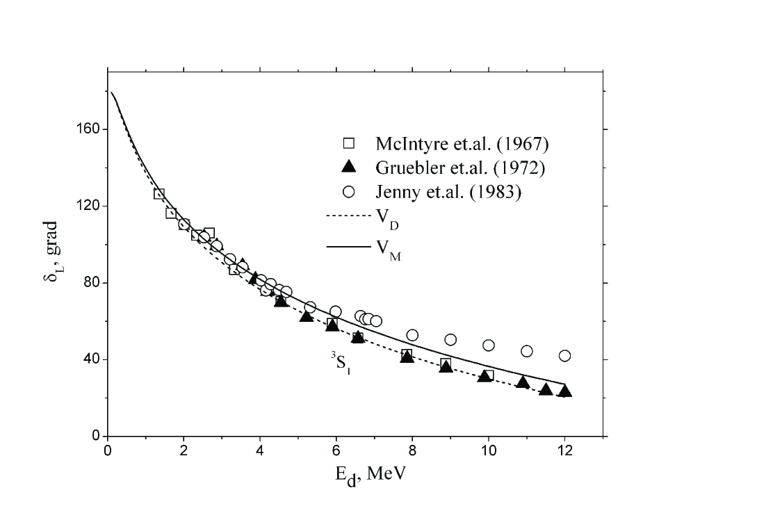
Figure 1: Phase shifts of the $\alpha+d$ elastic scattering in the S-wave with potentials $V_{D}$ and $V_{M}$ in comparison with the experimental data from Refs. mc67 ; grue75 ; jen83 .

The initial Gaussian potential in the ${}^{3}S_{1}$ wave $V_{D}(r)=-76.12\exp(-0.2r^{2})$ MeV dub94 describes well the phase shifts of the $\alpha-d$ scattering (see Fig. 1), however a consistence with the later data from the work jen83 is not so well.

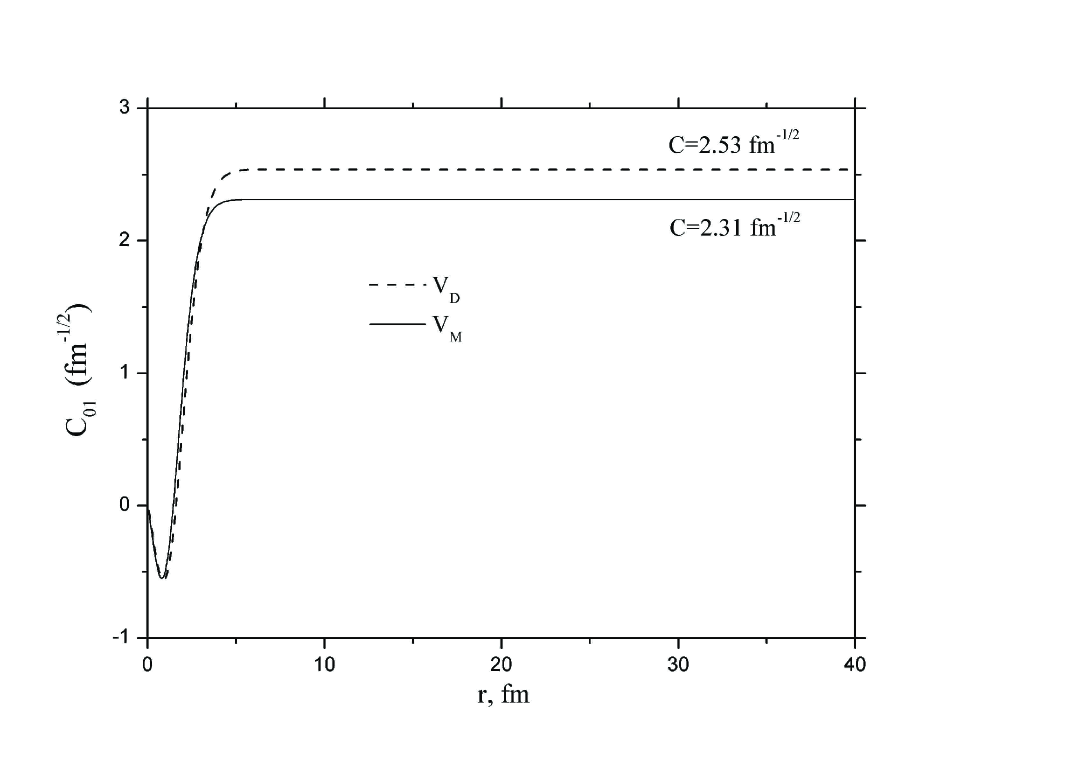
Figure 2: Asymptotics of the wave function of the $\alpha+d$ bound state in the S-wave, calculated with the potentials $V_{D}$ and $V_{M}$.

On Fig. 2 we give a description of the asymptotics of the bound state wave function of the $\alpha+d$ system. As can be seen from the figure, the calculated wave function on the base of the Numerov algorithm is well consistent with the asymptotics even with the number of mesh points $N=$200, which corresponds to $R_{max}=$ 10 fm. However, the initial potential $V_{D}(r)$ yields the estimation for the ANC of the $\alpha+d$ system with $C_{\alpha d}=2.53$ fm^-1/2, which is larger than the estimation from Ref. blok93 extracted from the experimental data on the $\alpha+d$ scattering by about 0.23 fm^-1/2. Therefore, in accordance with the ideology of Ref.mukh11 , we slightly modify the initial potential in such a way, that the resulting potential reproduces the correct value of ANC. On Fig.1 we also show the description of phase shifts in the S-wave with the modified potential $V_{M}(r)=-92.44\exp(-0.25r^{2})$ MeV, which are well consistent with the later data from Ref. jen83 . The same potential reproduces the empirical ANC with $C_{\alpha d}=2.31$ fm^-1/2 (see Fig. 2).

For the examination of the convergence of the theoretical results for the astrophysical S-factor and the differential cross section of the capture process ${}^{2}H(\alpha,\gamma)^{6}Li$, it is convenient to introduce an effective integral

$$I_{eff}(R,\lambda)=\left[Z_{1}\left(\frac{A_{2}}{A}\right)^{\lambda}+Z_{2}\left(\frac{-A_{1}}{A}\right)^{\lambda}\right]$$ (14)

$$\times\frac{1}{[(2\lambda+1)\textrm{!!}]}\sqrt{\frac{(\lambda+1)(2\lambda+1)}{\lambda}}\int^{R}_{0}u_{i}(r)(k_{\gamma}r)^{\lambda}u_{f}(r)dr,$$

the square of which is contained in the expression for the cross section at $R=\infty$. Thus, we can check a behavior of the effective integral with increasing $R$ at several energy values and with the fixed entrance channel and multiplicity $\lambda$ of the electric transition.

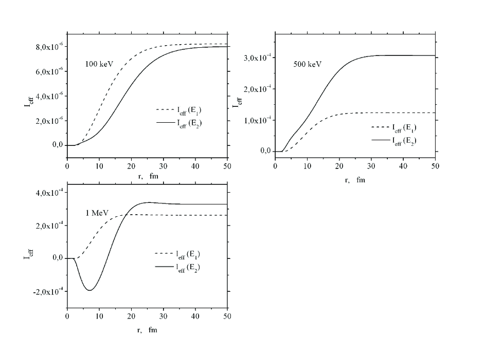
Figure 3: Convergence of the effective integrals $I_{eff}$ for E1(${}^{3}P_{2}->S$)- and E2(${}^{3}D_{3}->S$)- transitions at energies E=100 keV, E=500 keV, and E=1 MeV.

On Fig.3 we show effective integrals for the entrance channels ${}^{3}P_{2}$ and ${}^{3}D_{3}$, which give maximal contributions to the E1 and E2 transitions, correspondingly, at energies E=0.1, 0.5 and 1 MeV. From the figure one can see that the effective integrals for the E1 transition at all the energy values converge faster than the effective integrals for the E2 transition. For the E2 transition the convergence is achieved at 35-40 fm. Here it is important to note that at higher energies (for example at 1 MeV) the integrals for the E2 transition change the sign at 10-15 fm, which occurs due to the mutual cancellation of the internal and asymptotic parts of the transition matrix elements. At the same time, this situation is due to the presence of the extra Pauli forbidden state in the S-wave of the $\alpha+d$ two body system, that gives a node in the internal part of the ground state wave function. The mutual cancellation of the matrix elements allowed to reproduce data on the beta-transition of the ${}^{6}He$ halo nucleus into the $\alpha+d$ two-body continuum channel tur06 . At the end, in such cases the main contribution to the effective integrals comes from the asymptotic parts of the wave functions. For the E1 transition the wave functions of the entrance (P-wave) and exit (S-wave) channels have nodes due-to the Pauli forbidden states approximately at the same position, hence their product keeps the sign up to large distances. Therefore here one can not see any cancellation effects.

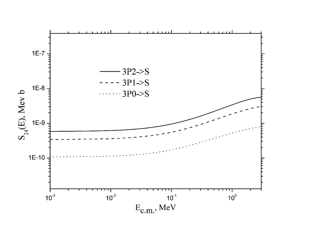
Figure 4: Contributions of the E1- components to the astrophysical S-factor for the synthesis reaction $\alpha+d\rightarrow^{6}Li+\gamma$ calculated with the potential $V_{M}$.

On Fig.4 the contributions from the partial waves to the E1-component of the astrophysical S-factor for the $\alpha+d\rightarrow^{6}Li+\gamma$ synthesis reaction calculated with the potential $V_{M}$ are demonstrated. As can be seen from the figure, the partial wave ${}^{3}P_{2}$ in the entrance channel yields the dominant contribution to the E1-transition.

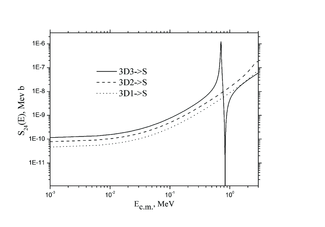
Figure 5: Contributions of the E2- components to the astrophysical S-factor for the synthesis reaction $\alpha+d\rightarrow^{6}Li+\gamma$ calculated with the potential $V_{M}$.

On Fig.5 we show the corresponding contributions from the partial waves to the E2-component of the astrophysical S-factor, calculated with the potential $V_{M}$. In this case, the dominant contribution to the process comes from the ${}^{3}D_{3}$ entrance channel in the energy interval up to the resonance region, and the maximal contribution behind the resonance comes from the ${}^{3}D_{2}$ entrance channel.

For the visual demonstration of the convergence of the obtained theoretical results, on Fig.6 we show the contributions of the E=E1+E2 transitions to the astrophysical S-factor for the capture reaction ${}^{2}H(\alpha,\gamma)^{6}Li$, estimated with the potential $V_{M}$ at several sets of mesh points with N=200, 400, 600, 800-2000 in the wide energy region. Since the step is fixed as $h=$0.05 fm, the respective upper limits of the integrals are 10, 20, 30, 40-100 fm. From the figure one can see that for the complete convergence it is necessary to choose the integral upper limit not less than 40 fm.

The contributions of the E1,E2, E1+E2 transitions to the astrophysical S-factor for the capture reaction $\alpha+d\rightarrow^{6}Li+\gamma$, estimated with the potentials $V_{M}$ and $V_{D}$ in comparison with the experimental data from Refs.mohr94 ; robe81 ; kien91 ; iga00 are shown on Fig.7. From the figure one can see that at low energies the main contribution to the astrophysical S-factor comes from the E1-component, and at energies around and behind the ${}^{3}D_{3}$ resonance region the contribution of the E2 component is dominant. We note also, that the initial potential $V_{D}$ from Ref.dub94 overestimates the experimental data in the region behind the resonance. But at low energies up to the resonance region the experimental data, as was noted above, are not well defined. Therefore it is too early to make a conclusion about the level of description of the data by the theoretical models at the low astrophysical energies. However, the theoretical results, obtained with the modified potential $V_{M}$ are very consistent with the results of Ref. mukh11 .

In the Table 1 we give our theoretical estimations for the reaction rates of the process $d(\alpha,\gamma)^{6}Li$ in the temperature interval $10^{6}K\leq T\leq 10^{10}K$ ($0.001\leq T_{9}\leq 10$) in comparison with the results of Refs. hamm10 ; mukh11 . In the second column we give ”the most effective energy” $E_{0}$, which gives the maximum to the integrant in Eq.(13). It is expressed as Angulo

$$E_{0}=\left(\frac{\mu}{2}\right)^{1/3}\left(\frac{\pi e^{2}Z_{1}Z_{2}k_{B}T}{\hbar}\right)^{2/3}=0.122\,(Z_{1}^{2}Z_{2}^{2}A)^{1/3}T_{9}^{2/3}\,\textrm{MeV,}$$ (15)

where $\mu$ is the reduced mass of the two particles. From the table one can find a good agreement of our results, obtained by using the modified potential $V_{M}$, with the results of Ref. mukh11 . However, our estimations are slightly lower than the results of the mentioned work. Probably, this is connected with the different potential choices and also with the fact that in Ref. mukh11 the asymptotical form of the $\alpha+d$ two-body wave function has been used for the estimation of the reaction rates at energies up to 350 keV.

IV Conclusions

The astrophysical S-factor and corresponding reaction rates for the process $d(\alpha,\gamma)^{6}Li$ have been estimated on the base of the two body model with the $\alpha-d$ potentials of a simple Gaussian form, which describe correctly the phase shifts in the partial waves ${}^{3}S_{1},\,^{3}P_{0},\,^{3}P_{1},\,^{3}P_{2},\,^{3}D_{1},\,^{3}D_{2},\,^{3}D_{3}$, and also the binding energy and ANC of the bound state in the S-wave. By modifying the S-wave potential from Ref. dub94 , we obtained a better description of the phase shifts and ANC, while keeping the binding energy of the ${}^{6}Li$ nucleus unchanged. For the calculations of the wave functions in the bound and continuum channels we have used the Numerov algorithm, which is of a high accuracy and yields the correct asymptotics of the wave function in the each partial wave. It was shown that a good convergence of the estimations for the contributions of the E1- and E2- transitions to the astrophysical S-factor is obtained when the upper limit of the integrals are extended up to 40 fm.

The theoretical results for the astrophysical S-factor and reaction rates of the process $d(\alpha,\gamma)^{6}Li$ in the temperature interval $10^{6}K\leq T\leq 10^{10}K$ ($0.001\leq T_{9}\leq 10$) are in a good agreement with the results of Ref. mukh11 , obtained by using known asymptotical form of the wave function at low energies and a complicated two-body potential at higher energies.

E.M.T. thanks Prof. L.D. Blokhintsev and Prof. B.F. Irgaziev for useful comments.

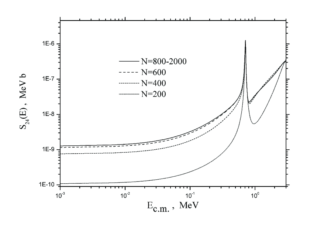
Figure 6: Contributions of the E1+E2 transitions to the astrophysical S-factor for the synthesis reaction $\alpha+d\rightarrow^{6}Li+\gamma$ calculated with the potential $V_{M}$ for different values of the mesh number N (convergence).

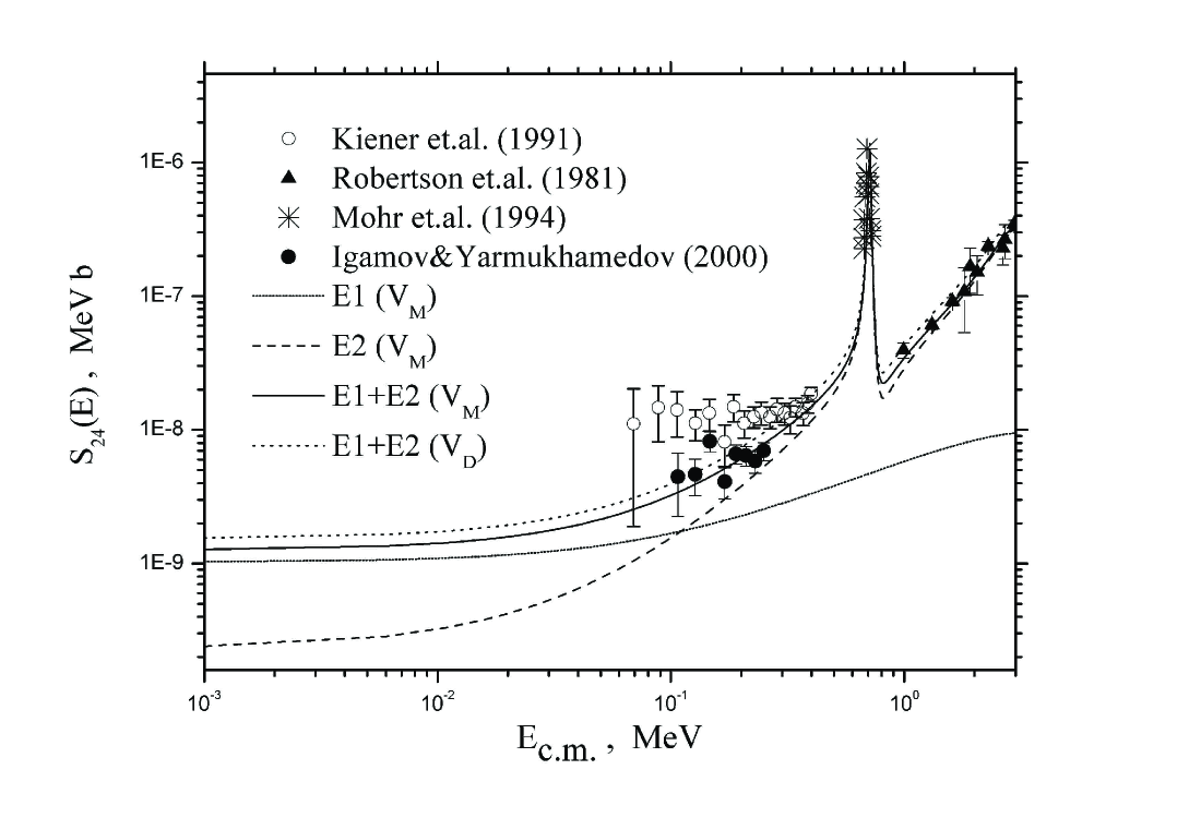
Figure 7: Contributions of the E1, E2, E1+E2 transitions to the astrophysical S-factor for the synthesis reaction $\alpha+d\rightarrow^{6}Li+\gamma$ calculated with the potentials $V_{M}$ and $V_{D}$ in comparison with the experimental data from Refs. robe81 ; kien91 ; mohr94 ; iga00 .

Table 1: Theoretical estimations for the reaction rates of the process $d(\alpha,\gamma)^{6}Li$ in the temperature interval $10^{6}K\leq T\leq 10^{10}K$ ($0.001\leq T_{9}\leq 10$) in comparison with the results of Refs. hamm10 ; mukh11 .

$T_{9}$	$E_{0}$	$N_{a}(\sigma v)$mukh11	$N_{a}(\sigma v)$hamm10	$N_{a}(\sigma v)$ ($V_{D}$)	$N_{a}(\sigma v)$ ($V_{M}$)
	(MeV)	$(\textrm{cm}^{3}$mol-1 c-1 )	( cm3 mol-1 c${}^{-1})$	$(\textrm{cm}^{3}$ mol-1 c-1 )	$(\textrm{cm}^{3}$ mol-1 c${}^{-1})$
		$C_{\alpha d}$=2.30 fm -1/2	$C_{\alpha d}$=2.70 fm -1/2	$C_{\alpha d}$=2.53 fm -1/2	$C_{\alpha d}$=2.31 fm -1/2
0.001	0.002	$6.467\times 10^{-30}$	$9.153\times 10^{-30}$	$6.730\times 10^{-30}$	$5.488\times 10^{-30}$
0.002	0.003	$1.857\times 10^{-23}$	$2.610\times 10^{-23}$	$2.012\times 10^{-23}$	$1.641\times 10^{-23}$
0.003	0.004	$2.470\times 10^{-20}$	$3.458\times 10^{-20}$	$2.729\times 10^{-20}$	$2.225\times 10^{-20}$
0.004	0.005	$2.286\times 10^{-18}$	$3.190\times 10^{-18}$	$2.557\times 10^{-18}$	$2.085\times 10^{-18}$
0.005	0.006	$5.693\times 10^{-17}$	$7.929\times 10^{-17}$	$6.426\times 10^{-17}$	$5.241\times 10^{-17}$
0.006	0.007	$6.592\times 10^{-16}$	$9.163\times 10^{-16}$	$7.492\times 10^{-16}$	$6.110\times 10^{-16}$
0.007	0.008	$4.651\times 10^{-15}$	$7.672\times 10^{-15}$	$5.315\times 10^{-15}$	$4.334\times 10^{-15}$
0.008	0.009	$2.327\times 10^{-14}$	$4.990\times 10^{-14}$	$2.671\times 10^{-14}$	$2.179\times 10^{-14}$
0.009	0.009	$9.067\times 10^{-14}$	$2.100\times 10^{-13}$	$1.045\times 10^{-13}$	$8.520\times 10^{-14}$
0.010	0.010	$2.923\times 10^{-13}$	$6.547\times 10^{-13}$	$3.379\times 10^{-13}$	$2.755\times 10^{-13}$
0.011	0.011	$8.127\times 10^{-13}$	$1.655\times 10^{-12}$	$9.422\times 10^{-13}$	$7.684\times 10^{-13}$
0.012	0.011	$2.008\times 10^{-12}$	$3.612\times 10^{-12}$	$2.334\times 10^{-12}$	$1.904\times 10^{-12}$
0.013	0.012	$4.508\times 10^{-12}$	$7.142\times 10^{-12}$	$5.251\times 10^{-12}$	$4.282\times 10^{-12}$
0.014	0.012	$9.343\times 10^{-12}$	$1.325\times 10^{-11}$	$1.091\times 10^{-11}$	$8.895\times 10^{-12}$
0.015	0.013	$1.811\times 10^{-11}$	$2.363\times 10^{-11}$	$2.119\times 10^{-11}$	$1.728\times 10^{-11}$
0.016	0.014	$3.318\times 10^{-11}$	$4.103\times 10^{-11}$	$3.887\times 10^{-11}$	$3.170\times 10^{-11}$
0.018	0.015	$9.676\times 10^{-11}$	$1.157\times 10^{-10}$	$1.137\times 10^{-10}$	$9.273\times 10^{-11}$
0.020	0.016	$2.432\times 10^{-10}$	$2.965\times 10^{-10}$	$2.865\times 10^{-10}$	$2.336\times 10^{-10}$
0.025	0.018	$1.538\times 10^{-09}$	$2.014\times 10^{-09}$	$1.822\times 10^{-09}$	$1.486\times 10^{-09}$
0.030	0.021	$6.277\times 10^{-09}$	$8.452\times 10^{-09}$	$7.462\times 10^{-09}$	$6.085\times 10^{-09}$
0.040	0.025	$4.870\times 10^{-08}$	$6.594\times 10^{-08}$	$5.823\times 10^{-08}$	$4.749\times 10^{-08}$
0.050	0.029	$2.093\times 10^{-07}$	$2.827\times 10^{-07}$	$2.512\times 10^{-07}$	$2.049\times 10^{-07}$
0.060	0.033	$6.375\times 10^{-07}$	$8.598\times 10^{-07}$	$7.672\times 10^{-07}$	$6.257\times 10^{-07}$
0.070	0.036	$1.554\times 10^{-06}$	$2.094\times 10^{-06}$	$1.874\times 10^{-06}$	$1.528\times 10^{-06}$
0.080	0.040	$3.245\times 10^{-06}$	$4.372\times 10^{-06}$	$3.921\times 10^{-06}$	$3.198\times 10^{-06}$
0.090	0.043	$6.057\times 10^{-06}$	$8.156\times 10^{-06}$	$7.327\times 10^{-06}$	$5.977\times 10^{-06}$
0.100	0.046	$1.038\times 10^{-05}$	$1.397\times 10^{-05}$	$1.257\times 10^{-05}$	$1.026\times 10^{-05}$
0.110	0.049	$1.665\times 10^{-05}$	$2.240\times 10^{-05}$	$2.018\times 10^{-05}$	$1.646\times 10^{-05}$
0.120	0.052	$2.533\times 10^{-05}$	$3.406\times 10^{-05}$	$3.072\times 10^{-05}$	$2.506\times 10^{-05}$
0.130	0.055	$3.690\times 10^{-05}$	$4.959\times 10^{-05}$	$4.476\times 10^{-05}$	$3.651\times 10^{-05}$
0.140	0.057	$5.185\times 10^{-05}$	$6.967\times 10^{-05}$	$6.292\times 10^{-05}$	$5.133\times 10^{-05}$
0.150	0.060	$7.071\times 10^{-05}$	$9.495\times 10^{-05}$	$8.582\times 10^{-05}$	$7.001\times 10^{-05}$
0.160	0.063	$9.398\times 10^{-04}$	$1.261\times 10^{-04}$	$1.141\times 10^{-04}$	$9.307\times 10^{-05}$
0.180	0.068	$1.559\times 10^{-04}$	$2.090\times 10^{-04}$	$1.892\times 10^{-04}$	$1.543\times 10^{-04}$
0.200	0.073	$2.416\times 10^{-04}$	$3.237\times 10^{-04}$	$2.932\times 10^{-04}$	$2.392\times 10^{-04}$
0.250	0.084	$5.868\times 10^{-04}$	$7.846\times 10^{-04}$	$7.112\times 10^{-04}$	$5.805\times 10^{-04}$
0.300	0.096	$1.167\times 10^{-03}$	$1.557\times 10^{-03}$	$1.412\times 10^{-03}$	$1.153\times 10^{-03}$
0.350	0.106	$2.040\times 10^{-03}$	$2.715\times 10^{-03}$	$2.461\times 10^{-03}$	$2.010\times 10^{-03}$
0.400	0.116	$3.256\times 10^{-03}$	$4.325\times 10^{-03}$	$3.916\times 10^{-03}$	$3.199\times 10^{-03}$
0.500	0.134	$6.930\times 10^{-03}$	$9.169\times 10^{-03}$	$8.258\times 10^{-03}$	$6.752\times 10^{-03}$
0.600	0.152	$1.271\times 10^{-02}$	$1.674\times 10^{-02}$	$1.484\times 10^{-02}$	$1.215\times 10^{-02}$
0.700	0.168	$2.148\times 10^{-02}$	$2.813\times 10^{-02}$	$2.414\times 10^{-02}$	$1.979\times 10^{-02}$
0.800	0.184	$3.462\times 10^{-02}$	$4.502\times 10^{-02}$	$3.816\times 10^{-02}$	$3.144\times 10^{-02}$
0.900	0.199	$5.385\times 10^{-02}$	$6.944\times 10^{-02}$	$6.213\times 10^{-02}$	$5.191\times 10^{-02}$
1.000	0.213	$8.079\times 10^{-02}$	$1.033\times 10^{-01}$	$9.209\times 10^{-02}$	$7.755\times 10^{-02}$
1.500	0.279	$3.508\times 10^{-01}$	$4.350\times 10^{-01}$	$3.840\times 10^{-01}$	$3.312\times 10^{-01}$
2.000	0.338	$7.854\times 10^{-01}$	$9.623\times 10^{-01}$	$8.456\times 10^{-01}$	$7.342\times 10^{-01}$
2.500	0.393	$1.268\times 10^{+00}$	$1.549\times 10^{+00}$	$1.356\times 10^{+00}$	$1.177\times 10^{+00}$
3.000	0.443	$1.745\times 10^{+00}$	$2.132\times 10^{+00}$	$1.858\times 10^{+00}$	$1.609\times 10^{+00}$
4.000	0.537	$2.673\times 10^{+00}$	$3.280\times 10^{+00}$	$2.839\times 10^{+00}$	$2.438\times 10^{+00}$
5.000	0.623	$3.631\times 10^{+00}$	$4.476\times 10^{+00}$	$3.895\times 10^{+00}$	$3.321\times 10^{+00}$
6.000	0.704	$4.645\times 10^{+00}$	$5.754\times 10^{+00}$	$5.056\times 10^{+00}$	$4.291\times 10^{+00}$
7.000	0.780	$5.689\times 10^{+00}$	$7.088\times 10^{+00}$	$6.271\times 10^{+00}$	$5.309\times 10^{+00}$
8.000	0.853	$6.725\times 10^{+00}$	$8.438\times 10^{+00}$	$7.501\times 10^{+00}$	$6.342\times 10^{+00}$
9.000	0.922	$7.723\times 10^{+00}$	$9.773\times 10^{+00}$	$8.707\times 10^{+00}$	$7.354\times 10^{+00}$
10.00	0.989	$8.664\times 10^{+00}$	$1.107\times 10^{+01}$	$9.864\times 10^{+00}$	$8.325\times 10^{+00}$

References

• (1) P.D.Β  Serpico et al., J. Cosmol. Astropart. Phys. 12, 010 (2004).
• (2) P.Β  Mohr et al., Phys. Rev. C 50, 1543 (1994).
• (3) R.G.H.Β  Robertson et al., Phys. Rev. Lett. 47, 1867 (1981).
• (4) J.Β  Kiener et al., Phys. Rev. C44, 2195 (1991).
• (5) F.Β  Hammache et al., Phys. Rev. C 82, 065803 (2010).
• (6) K.Β  Langanke, Nucl. Phys. A 457, 351 (1986).
• (7) S.Β  Typel, H.H.Β  Wolter, and G.Β Baur, Nucl. Phys. A613, 147 (1997).
• (8) A.Β  Kharbach and P.Β  Descouvemont, Phys. Rev. C 58, 1066 (1998).
• (9) S.B.Β Dubovichenko, A.V.Β Dzhazairov-Kahramanov, Yadernaya Fizika 58, 635 (1995); 852 (1995).
• (10) K.M.Β  Nollett, R.B.Β Wiringa, and R.Β  Shiavilla, Phys. Rev. C 63, 024003 (2001).
• (11) A.M.Β  Mukhamedzhanov, L.D.Β  Blokhintsev, and B.F.Β  Irgaziyev, Phys. Rev. C 83, 055805 (2011).
• (12) L.D.Β  Blokhintsev, V.I.Β  Kukulin, A.A.Β  Sakharuk, D. A.Β  Savin, E.V.Β  Kuznetsova, Phys. Rev. C 48, 2390 (1993).
• (13) S.B.Β Dubovichenko, Yadernaya Fizika, 73, 1573 (2010).
• (14) S.B.Β Dubovichenko, A.V.Β Dzhazairov-Kahramanov, Yadernaya Fizika, 57, 784 (1994).
• (15) Tao Pang, An Introduction to Computational Physics, (Cambridge University Press, 2010), 402 p.
• (16) B. Jenny et al., Nucl. Phys. A397, 61 (1983)
• (17) L.C. McIntyre and W. Haeberli, Nucl.Phys.A91, 382 (1967)
• (18) W. Gruebler et.al., Nucl.Phys.A242, 265 (1975)
• (19) C. Angulo et.all., Nucl. Phys. A 656 (1999) 3
• (20) W.A. Fowler, G.R. Gaughlan, and B.A. Zimmerman, Ann. Rev. Astron. Astrophys. 13 (1975) 69
• (21) E.M.Β Tursunov, D.Β Baye and P.Β Descouvemont, Phys. Rev. C73, 014303 (2006).
• (22) S.B. Igamov and R. Yarmukhamedov, Nucl. Phys. A 673 (2000) 509
Refer to caption