Optimal control of quantum gates in an exactly solvable non-Markovian open quantum bit system

Abstract

We apply quantum optimal control theory (QOCT) to an exactly solvable non-Markovian open quantum bit (qubit) system to achieve state-independent quantum control and construct high-fidelity quantum gates for moderate qubit decaying parameters. An important quantity, improvement $\mathcal{I}$, is proposed and defined to quantify the correction of gate errors due to the QOCT iteration when the environment effects are taken into account. With the help of the exact dynamics, we explore how the gate error is corrected in the open qubit system and determine the conditions for significant improvement. The model adopted in this paper can be implemented experimentally in realistic systems such as the circuit QED system.

I Introduction

Quantum optimal control theory (QOCT) which incorporates the optimal control theory with the quantum theory is a powerful tool and has attained various physical achievements Peirce et al. (1988); Kosloff89 ; TannorBook ; PhysRevLett.89.188301 ; Montangero et al. (2007); Maximov et al. (2008); Spörl et al. (2007); Tsai et al. (2009); Eitan et al. (2011); Brif10 . It has also been introduced to quantum gate control to obtain the optimal control pulses in quantum gate operations. In the literature, quantum gate control employing QOCT in closed or open systems are studied PhysRevLett.89.188301 ; Montangero et al. (2007); Spörl et al. (2007); Tsai et al. (2009); JPhysB.40.S75 ; Rebentrost et al. (2009); Wenin and Pötz (2008a); *PhysRevB.78.165118; *wenin:084504; *PhysRevB.79.224516; *PhysRevA.74.022319; Jirari (2009); Gordon et al. (2008); Clausen et al. (2010); Hwang and Goan (2012). However, in most investigations where the environment effect is taken into account, the dynamics are often derived perturbatively, involving Born Breuer and Petruccione (2002); Breuer et al. (1999); Meier99 ; Breuer01 ; Yan98 ; Schroder06 ; Ferraro09 ; Shibata77 ; Kleinekathofer04 ; Liu07 ; Sinayskiy09 ; Mogilevtsev09 ; Haikka10 ; Ali10 ; Chen11 ; Goan11 or Born-Markov approximations Scully97 ; Carmichael (1998); Gardiner00 ; Barnett02 ; Milburn08 . Despite the broad applicability of the perturbative master equation, the approximations made in the derivation results in unwanted intrinsic error, which in turn contributes to the gate error as the pulse sequence for the gate operation is obtained through the approximated master equation. In cases where the models can be exactly solved, resorting to the exact dynamics can help reduce these possible intrinsic errors.

In this paper, we adopt an exact master equation of a qubit Breuer and Petruccione (2002); PhysRevA.54.R3750 ; Garraway (1997); Diósi et al. (1998) and combine it with QOCT based on the Krotov iteration method Krotov (1996); TannorBook ; PhysRevLett.89.188301 ; Maximov et al. (2008); Sklarz and Tannor (2002) to find the optimal control pulse for state-independent single-qubit gate control in a general non-Markovian environment with an arbitrary spectral density. To be specific, the model we consider is a qubit linearly coupled to a dissipative zero-temperature environment through a qubit lowering operator $\sigma_{-}$. The exact master equation for this model can be derived from either the pseudo mode method Garraway (1997); Breuer and Petruccione (2002) or the quantum state diffusion equation Diósi et al. (1998); Diósi and Strunz (1997); *PhysRevLett.82.1801; *PhysRevLett.74.203. Reasonable trends of gate error for this model under various conditions are observed and discussed. Moreover, if the bath spectral density is chosen to be a Lorentzian type, this dissipative qubit model can be shown to be equivalent to the damped Jaynes-Cummings model describing the coupling of a qubit to a single cavity mode which in turn is coupled to a Markovian reservoir Garraway (1997); Breuer and Petruccione (2002). Thus our optimal control results would also have direct applications, for example, to superconducting circuit quantum electrodynamic (QED) systems Blais et al. (2004); Wallraff et al. (2004); Circuit_QED_review ; Sarovar05 that are described very well by the damped Jaynes-Cummings model and are controlled relatively easily by external fields.

Another important property we wish to investigate is whether or not in open systems, QOCT is able to correct the gate error due to the environment effect. A quantity, improvement $\mathcal{I}$, is defined to quantify such correction. For a system where the improvement is large, including the environment effect becomes essential to the control problem. Whereas for a system with negligible improvement, the optimal control pulse developed while the system is considered closed would suffice. We further explore the region of parameters where significant improvement is achieved, and find that improvement is in close relation to the structure of the environment. We note here that in cases where the open quantum system models are not exactly solvable, one will have to turn to the perturbative master equation approaches for the optimal control solution JPhysB.40.S75 ; Rebentrost et al. (2009); Wenin and Pötz (2008a); *PhysRevB.78.165118; *wenin:084504; *PhysRevB.79.224516; *PhysRevA.74.022319; Jirari (2009); Gordon et al. (2008); Clausen et al. (2010); Hwang and Goan (2012). However, in certain models where the exact master equations are available, our present treatment bears the advantage of ruling out the intrinsic errors due to the perturbative dynamics.

II Model and method

II.1 Model and exact master equation

Only a few non-Markovian open quantum system models can be exactly solved Garraway (1997); Piilo et al. (2008); Imamoglu (1994); Breuer et al. (1999); Hu et al. (1992); Tu08 ; Goan10 ; Jing and Yu (2010); Diósi et al. (1998), and exact dissipative models of a two-level system are even fewer. The total Hamiltonian $H_{\text{tot}}$ of the two-level qubit model we consider consists of three parts Diósi et al. (1998); Garraway (1997); Breuer and Petruccione (2002) (set $\hbar=1$):

$$H_{\text{qbit}}=\frac{\omega_{0}}{2}\sigma_{z},$$

$$H_{\text{bath}}=\sum_{\lambda}\omega_{\lambda}a_{\lambda}^{\dagger}a_{\lambda},$$

$$H_{\text{int}}=\sum_{\lambda}(g_{\lambda}^{*}La_{\lambda}^{\dagger}+g_{\lambda}L^{\dagger}a_{\lambda}).$$ (1)

Here $\omega_{0}$ is the qubit transition frequency; $\sigma_{z}$ is the Pauli-$Z$ matrix; and $a_{\lambda}$, $a_{\lambda}^{\dagger}$ are the creation and annihilation operator for the bath oscillator with eigenfrequency $\omega_{\lambda}$. In this exactly solvable model, the qubit is linearly coupled to the zero-temperature environment through the Lindblad operator $L=\sigma_{-}$ with coupling constant $g_{\lambda}$. We choose the qubit transition frequency as the time-dependent control parameter, $\omega_{0}\rightarrow\omega_{0}+\epsilon(t)\equiv\omega_{0}(t)$. In real experiments, $\omega_{0}$ is often tunable and is a possible agent of external control. The exact master equation reads Diósi et al. (1998); Garraway (1997); Breuer and Petruccione (2002)

$$\dot{\rho}(t)=-\frac{i\omega_{0}(t)}{2}\left[\sigma_{z},\rho(t)\right]+2\text{Re}\left[F(t)\right]$$

$$\times\left(\sigma_{-}\rho(t)\sigma_{+}-\frac{1}{2}\left\{\sigma_{+}\sigma_{-},\rho(t)\right\}\right)+i\text{Im}\left[{F(t)}\right]\left[\sigma_{+}\sigma_{-},\rho(t)\right],$$ (2)

where $\text{Re}[\cdots]$ and $\text{Im}[\cdots]$ stand for the real and imaginary parts of a complex function,

$$F(t)=\int_{0}^{t}c(t,s)f(t,s)ds$$ (3)

satisfying the differential equation

$$\partial_{t}f(t,s)=\{i\left(\omega_{0}+\epsilon(t)\right)+F(t)\}f(t-s)$$ (4)

and the bath correlation function is defined as

$$c(t-s) \equiv\sum_{\lambda}\left|g_{\lambda}\right|^{2}e^{-i\omega_{\lambda}(t-s)}$$

$$\rightarrow\int_{0}^{\infty}d\omega J(\omega)e^{-i\omega(t-s)},$$ (5)

where we have taken the continuum limit and $J(\omega)$ is the environment spectral density. Equation (4) is a nonlocal integro-differential equation and is not easy to solve for a general bath spectral density and thus to incorporate within the framework of QOCT. One important observation to deal with this time-nonlocal equation is to express the bath correlation function in a multi-exponential form Meier99 ; Yan01 ; Kleinekathofer04 ; Kleinekathofer06 ; Hwang and Goan (2012),

$$c(t-s)=\sum_{j}p_{j}e^{q_{j}(t-s)}=\sum_{j}c_{j}(t-s),$$ (6)

where $p_{j}$ and $q_{j}$ are complex constants and can be found by numerical methods. Then we see from Eqs. (3) and (4) that the relevant function $F(t)$ in Eq. (II.1) satisfies $F(t)=\sum_{j}F_{j}(t)$ and

$$\partial_{t}F_{j}(t)= p_{j}+F_{j}(t)\left[q_{j}+i\left[\omega_{0}+\epsilon(t)\right]+\sum_{k\neq j}F_{k}(t)\right]$$

$$+ F_{j}^{2}(t),$$ (7)

along with the initial condition $F_{j}(0)=0$. Equation (II.1) forms a set of coupled time-local equations that yield a simple, fast and stable iterative scheme to incorporate with the Krotov QOCT method that we will employ. For the convenience of numerical computation, we treat the density matrix as a column vector $\rho^{c}$ and Eq. (II.1) can be put in the form $\dot{\rho}^{c}(t)=\Lambda(t)\rho^{c}(t)$. The propagator $\mathcal{G}(t)$ is defined such that $\rho^{c}(t)=\mathcal{G}(t)\rho^{c}(0)$ and can be viewed as a state-independent gate operation. The differential equation for $\mathcal{G}(t)$ is $\dot{\mathcal{G}}(t)=\Lambda(t)\mathcal{G}(t)$ and $\mathcal{G}(t)$ is identity when $t=0$.

II.2 Krotov’s method of optimal control theory

In QOCT, it is necessary to define a quantity, or the cost function, we wish to maximize or minimize after each iteration Krotov (1996); TannorBook ; PhysRevLett.89.188301 ; Maximov et al. (2008); Sklarz and Tannor (2002). In open system gate control, this quantity corresponds to the gate error defined at the final gating time $t_{f}$ Maximov et al. (2008); Wenin and Pötz (2008a); *PhysRevB.78.165118; *wenin:084504; *PhysRevB.79.224516; *PhysRevA.74.022319,

$$\mathcal{E}\equiv\frac{1}{2\mathcal{N}}\text{Tr}\left\{[\mathcal{O}-\mathcal{G}(t_{f})]^{\dagger}[\mathcal{O}-\mathcal{G}(t_{f})]\right\},$$ (8)

where $\mathcal{O}$ is the control target to be specified and $\mathcal{N}$ is the dimension of $\mathcal{G}(t)$ in the column vector representation. This error $\mathcal{E}$ or fidelity $(1-\mathcal{E})$ definition can be mapped to the trace fidelity commonly used in closed systems when the dynamics becomes unitary. For the dissipative two-level model with control over the $\sigma_{z}$ term, we perform $Z$-gate and identity gate control. For the $Z$-gate control, the target $\mathcal{O}_{z}$ in the column vector representation is defined as $\text{diag}\left(1,-1,-1,1\right)$ and for identity-gate control $\mathcal{O}_{I}=I_{\mathcal{N}}$, where $I_{\mathcal{N}}$ is the identity matrix in the column vector representation.

The update algorithm of the optimization iteration based on the Krotov method is as follows Krotov (1996); TannorBook ; PhysRevLett.89.188301 ; Maximov et al. (2008); Hwang and Goan (2012): (1) An admissible initial control $\epsilon^{0}(t)$ is constructed either by guess or experience. Find the trajectory $\mathcal{G}^{(0)}(t)$ by intergrating the equation of motion along with the initial condition using the control $\epsilon^{(0)}$. (2) An auxiliary backward propagator $\chi(t)$ is found by integrating the differential equation $\dot{\chi}(t)=\Lambda^{\dagger}\chi(t)$ with its boundary condition $\chi(t_{f})=[\mathcal{O}-\mathcal{G}(t_{f})]/2\mathcal{N}$. (3) Solve the equation of motion for $\mathcal{G}(t)$ and the control update rule

$$\epsilon=\epsilon^{(0)}+2\lambda\mbox{Re}\left(\mbox{Tr}\left[\chi^{\dagger}\left.\frac{\partial\Lambda}{\partial\epsilon}\right|_{\epsilon^{(0)}}\mathcal{G}\right]\right)$$

self-consistently to yield the updated control and propagator $\epsilon^{(1)}$ and $\mathcal{G}^{(1)}$ for a small enough $\lambda$ to ensure the monotonic convergence of the algorithm. (4) Substitute $\epsilon^{(1)}$ and $\mathcal{G}^{(1)}$ for $\epsilon^{(0)}$ and $\mathcal{G}^{(0)}$ in step (1) and repeat steps (1) to (3) until the error converges to a saturated value (a preset error threshold is reached or a given number of iterations has been performed).

We constrain the control parameter—in our case the time-dependent transition frequency—to an allowable range. In real experiments, there exists an attainable range of qubit frequency determined by the external control agent and the physical system. Beyond this range, the control is unattainable or simply destroys the original system. An example can be the critical magnetic field in the superconducting circuit QED system Tinkham (2004); Blais et al. (2004); Wallraff et al. (2004); Circuit_QED_review ; Sarovar05 . Thus for most of the results presented here, we set the range to be $0\leq\omega_{0}(t)\leq 2\omega_{0}$, i.e., $\left|\epsilon(t)\right|\leq\omega_{0}$. The value of $\omega_{0}$ is determined by the actual physical system implementing this model. We will present results with large range control $\left|\epsilon(t)\right|\leq 20\omega_{0}$ in Sec. III.3.

II.3 Improvement

In our model, the optimal pulses for $Z$-gates and identity gates in closed systems can be obtained straightforwardly. An important question to be addressed is, how much can QOCT improve the gate fidelity in an open quantum system, given that we take the ideal closed system optimal pulse as our initial guess. For a fixed gating time $t_{f}$ and a constant magnitude control pulse, $\omega_{0}(t)=\omega_{0}+\epsilon(t)=n\pi/t_{f}$ where $n$ is even for the identity gate and odd for the $Z$-gates. We take this ideal closed system pulse as the initial guess for optimal control in open systems. Define the quantity, improvement $\mathcal{I}$:

$${\mathcal{I}\equiv\log_{10}{\left(\frac{E^{(0)}}{E^{(s)}}\right)}},$$ (9)

where $E^{(0)}$ denotes the gate error before the QOCT iteration, and $E^{(s)}$ is the saturated gate error after the iteration. Improvement characterizes the order of magnitude of the gate error improved by the QOCT iteration.

III Numerical results and discussion

In principle, we can deal with any environment spectral density resulting in a bath correlation function that can be expanded in the form of a multi-exponential function. Here we consider two kinds of environment spectral densities or environment correlation functions: the Lorentzian-like correlation function and the Ohmic correlation function. The Lorentzian spectral density $J_{l}(\omega)=\frac{\alpha}{2\pi}\frac{\gamma^{2}}{(\omega-\Omega)^{2}+\gamma^{2}}$ yields the Lorentzian-like exponential decaying bath correlation function Breuer and Petruccione (2002); Garraway (1997); Lor

$${c_{l}(t-s)=\alpha\frac{\gamma}{2}\exp\left[-\gamma|t-s|-i\Omega(t-s)\right]}.$$ (10)

The environment effect is characterized by the correlation strength $\alpha$, the correlation time $\gamma^{-1}$, and the central frequency of the environment spectrum $\Omega$. The Ohmic correlation function can be derived analytically from the Ohmic spectral density $J_{o}(\omega)=2\alpha_{o}\omega\exp{(-\omega/\omega_{c})}$ as Leggett et al. (1987)

$${c_{o}(t-s)=2\alpha_{o}\omega_{c}^{2}\left[1+i\omega_{c}(t-s)\right]^{-2}},$$ (11)

where $\alpha_{o}$ is the dimensionless coupling strength and $\omega_{c}$ is the cutoff frequency. Note that function fitting is required to put Eq. (11) in a multi-exponential form. We present below the numerical results with the parameters in units of $\omega_{0}$ if not stated otherwise.

III.1 Numerical results

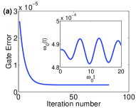
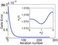
Figure 1: (Color online) Typical QOCT iteration profile and control pulses in the Lorentzian-like environment. (a) Identity-gate control with $\alpha=0.01$, $\gamma=0.1$, $\Omega=1$, and $t_{f}=20$. (b) $Z$-gate control with $\alpha=0.1$, $\gamma=0.1$, $\Omega=5$, and $t_{f}=2$.

Figure 1 shows typical optimal pulses (in the insets) and the monotonic converging behavior of the QOCT iteration, a favorable feature of the Krotov method, and the saturation of gate error near the optimal trajectory. The smooth shape of the optimal control pulses can be easily engineered. Identity gates serve as quantum memories and thus favor long gating times. Figure 2 shows the gate error after QOCT iteration and improvement vs gating time of the identity-gate control in both the Lorentzian-like environment [Figs. 2(a) and 2(b)] and the Ohmic environment [Figs. 2(c) and 2(d)]. It appears that high-fidelity identity gates with error $\mathcal{E}\lesssim 10^{-3}$ can be achieved for gating times longer than the system decay time for moderate system decay parameters. Gate control is better performed with weaker qubit-environment coupling strength ($\alpha$ or $\alpha_{o}$ small) and with smaller $\gamma$ or $\omega_{c}$ in both cases. Note that improvement increases as the gating time gets longer. The anomalous crossing in Fig. 2(d) results from gate error saturation in extreme conditions. A $Z$-gate operation is desired to be fast and thus requires a short gating time. We set a fixed $Z$-gate gating time $t_{f}=2\omega_{0}^{-1}$, which is the smallest multiples of $\omega_{0}^{-1}$ within which an ideal closed system $Z$-gate can be fulfilled in the admissible control range. The results are shown in Tables 1 and 2. The trends are similar to the identity-gate control.

The parameters $\gamma$ and $\omega_{c}$ determine the bath correlation time and the shape of the correlation function. From Eqs. (10) and (11), it can be shown that larger $\gamma$ or $\omega_{c}$ corresponds to a bath correlation function of shorter correlation time and a stronger correlation strength near $s=t$, namely, a relatively Markovian correlation. In Table 1, we demonstrate the effect of $\Omega$ on $Z$-gate control. The gate error becomes smaller when $\Omega$ increases. Mathematically, this can be inferred from Eq. (10) that large $\Omega$ results in mutual cancellation of the bath correlation function in, for example, the integration of Eq. (3) and thus minor environment effect. Physically, the peak of the spectral density is detuned away from the qubit frequency by large $\Omega$ and results in weak environment-induced decoherence.

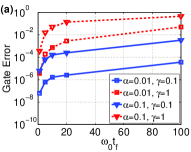
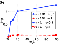
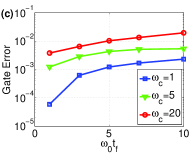
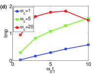
Figure 2: (Color online) Gate error and improvement vs gating time of identity-gate control. (a) and (b) correspond to a Lorentzian-like environment with $\Omega=1$, and (c) and (d) correspond to an Ohmic environment with $\alpha_{o}=0.01$.

Figures 3(a)–3(c) show the plots of the improvement of $Z$-gate control under various conditions in Lorentzian environment. Apparently there is hardly any improvement when $\Omega$ is in the vicinity of the system transition frequency. As the detuning $(\Omega-\omega_{0})$ grows large, we observe great improvement in the $Z$-gate control. The increase in the improvement is not monotonic. In the Ohmic environment [Fig. 3(d)], the improvement grows with the cutoff frequency $\omega_{c}$ as in the identity-gate control [Fig. 2(d)]. In all cases, neither $\alpha$ nor $\alpha_{o}$ plays a role in improvement. To study the trend of improvement, we shall study the exact dynamics and explore the agent of error correction in the QOCT iteration for the dissipative system we investigate.

Table 1: Errors of the $Z$-gate control in a Lorentzian-like environment under various conditions.

$\Omega=\omega_{0}$
$\alpha$	$\gamma=0.1$	$\gamma=1$	$\gamma=10$
0.01	$8.89\times 10^{-7}$	$3.53\times 10^{-5}$	$1.10\times 10^{-4}$
0.1	$8.81\times 10^{-5}$	$3.31\times 10^{-3}$	$9.57\times 10^{-3}$
1	$8.06\times 10^{-3}$	$1.78\times 10^{-1}$	$2.86\times 10^{-1}$
$\Omega=5\omega_{0}$
$\alpha$	$\gamma=0.1$	$\gamma=1$	$\gamma=10$
0.01	$5.17\times 10^{-10}$	$1.40\times 10^{-6}$	$9.15\times 10^{-5}$
0.1	$5.18\times 10^{-8}$	$1.37\times 10^{-4}$	$7.98\times 10^{-3}$
1	$5.35\times 10^{-6}$	$1.10\times 10^{-2}$	$2.59\times 10^{-1}$
$\Omega=10\omega_{0}$
$\alpha$	$\gamma=0.1$	$\gamma=1$	$\gamma=10$
0.01	$1.54\times 10^{-10}$	$5.63\times 10^{-8}$	$4.16\times 10^{-5}$
0.1	$1.54\times 10^{-8}$	$5.60\times 10^{-6}$	$3.79\times 10^{-3}$
1	$1.57\times 10^{-6}$	$5.31\times 10^{-4}$	$1.67\times 10^{-1}$

Table 2: Errors of the $Z$-gate control in an Ohmic environment under various conditions.

$\alpha_{o}$	$\omega_{c}=1$	$\omega_{c}=5$	$\omega_{c}=20$
$10^{-4}$	$9.73\times 10^{-8}$	$1.97\times 10^{-6}$	$4.64\times 10^{-6}$
$10^{-3}$	$9.70\times 10^{-6}$	$1.93\times 10^{-4}$	$4.52\times 10^{-4}$
$10^{-2}$	$9.40\times 10^{-4}$	$1.58\times 10^{-2}$	$3.22\times 10^{-2}$

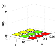
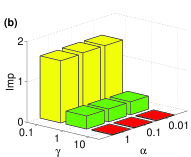
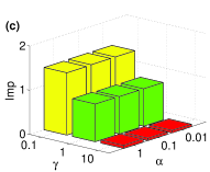
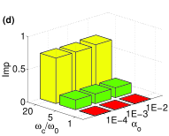
Figure 3: (Color online) Improvement under various conditions of $Z$-gate control. (a)–(c) are plotted with $\Omega=1$, 5, and 10, respectively, in a Lorentzian-like environment and (d) in an Ohmic environment.

III.2 Conditions for significant improvement

In the previous section we have shown that in both Lorentzian-like and Ohmic environments, improvement $\mathcal{I}$ of gate control varies largely as the qubit-decaying parameters are tuned. We now explore the conditions under which significant improvement happens and discuss the physics behind them for the exactly solvable dissipative model we consider.

The coherence term ($\rho_{21}$, in particular) of the exact solution to Eq. (II.1) suggests that $\text{Re}\left[\int_{0}^{t}F(s)ds\right]$ encodes the dissipation caused by the environment, and $\text{Im}\left[\int_{0}^{t}F(s)ds\right]$ encodes the phase shift of the coherence term resulting from the shift in the system frequency due to the presence of the environment. It reads

$$\rho_{21}(t)= \rho_{21}(0)\exp\left(-\int_{0}^{t}\text{Re}\left[F(s)\right]ds\right)$$

$$\times\exp\left(i\left(\int_{0}^{t}\omega_{0}(s)ds+\int_{0}^{t}\text{Im}\left[F(s)\right]ds\right)\right)$$

$$\equiv \rho_{21}(0)e^{-\kappa}e^{i\phi}.$$ (12)

The first exponential term represents the dissipation effect ($\kappa$) and the second represents the phase shift ($\phi$). It is desirable to check how $\kappa$ and $\phi$ behave before and after the QOCT iteration. A quick check in the exponents of several typical cases shows that the phase shift ($\phi$) is corrected by the QOCT iteration as shown in Table 3; the dissipation ($\kappa$), however, can hardly be suppressed. This is because in the exactly solvable dissipative model considered here, the control is only over the $\sigma_{z}$ term that enables the explicit phase correction, and the control strength is not very strong ($\left|\epsilon(t)\right|\leq\omega_{0}$) for the cases investigated here (note that the dissipation can be substantially suppressed with large range control $\left|\epsilon(t)\right|\leq 20\omega_{0}$ shown in Sec. III.3). As a consequence, improvement is determined by the relative proportion of error that the two effects of the phase shift and the dissipation contribute to. In our dissipative model with control only on the $\sigma_{z}$ term, if the environment-induced dissipation is the dominant source of gate error, the improvement is limited since after the optimal control iteration, only a minor portion of error can be corrected. In contrast, if the gate error mainly comes from the environment-induced phase shift, then after the optimal control iteration the improvement can be substantial.

Table 3: The phase shift exponent $\phi$ and dissipation exponent $\kappa$. The superscripts $(0)$ and $(s)$ indicate the values taken before and after the QOCT iteration, respectively.

	Case 1	Case 2	Case 3	Case 4
$\kappa^{(0)}$	$2.04\times 10^{-4}$	$8.46\times 10^{-3}$	$1.90\times 10^{-2}$	$2.79\times 10^{-3}$
$\kappa^{(s)}$	$2.04\times 10^{-4}$	$8.46\times 10^{-3}$	$1.93\times 10^{-2}$	$2.79\times 10^{-3}$
$\phi^{(0)}$	$-8.63\times 10^{-4}$	$1.04\times 10^{-3}$	$-2.71\times 10^{-2}$	$-4.61\times 10^{-5}$
$\phi^{(s)}$	$-6.66\times 10^{-8}$	$2.91\times 10^{-5}$	$-1.36\times 10^{-4}$	$3.32\times 10^{-9}$
$\mathcal{I}$	$1.50$	$0.0141$	$0.693$	$0.000447$

The dissipation and the phase shift are directly related to the nature of $F(t)$, which is determined by its differential equation, Eq. (II.1). Mathematically, it is possible to find conditions such that the gate error contributed by $\left|\int_{0}^{t_{f}}\text{Im}\left[F(s)\right]ds\right|$ is relatively larger than that by $\left|\int_{0}^{t_{f}}\text{Re}\left[F(s)\right]ds\right|$ and thus determine the conditions for significant improvement.

Physically, the effect of phase shift and dissipation can be understood as the result of qubit transition frequency shift, namely, Lamb shift, and qubit decay. In the Lorentzian environment with zero detuning, $\Omega=\omega_{0}$, the spectral density is peaked at and symmetric with respect to $\omega_{0}$. As the numerical results indicate, the decay rate becomes large and the dissipation effect becomes prominent. On the other hand, the Lamb shift is relatively small due to the symmetric distribution of spectral density with respect to qubit frequency $\omega_{0}$. In this case the dissipation effect dominates over the phase shift effect, and the improvement due to the optimal control is small.

However, if the environment central frequency is detuned from the qubit frequency, our numerical results indicate that qubit decay drops dramatically, but the Lamb shift does not change much. This is due to the asymmetric distribution of the spectral density with respect to qubit frequency $\omega_{0}$ and the result consequently leads to significant improvement. This is in agreement with the trend of improvement observed in the previous sections. Note that this behavior is more prominent as the Lorentzian distribution gets narrower ($\gamma$ small). Similar arguments apply to the Ohmic case. The overall coupling strength $\alpha$ (or $\alpha_{o}$) is irrelevant to the improvement since it does not affect the shape of the spectral density but only the overall value.

III.3 Suppression of dissipation

So far, we have observed very limited suppression of dissipation applying QOCT to the two-level dissipative model. This consequence is model specific, and is due to the control range we specify. In Eq. (III.2), the control pulse can be designed to directly cancel the environment-induced phase shift, but can hardly suppress the dissipation effect through minimizing the magnitude of $\text{Re}\left[\int_{0}^{t_{f}}[F(s)]ds\right]$. However, one can observe in Eq. (II.1) that $\epsilon(t)$ follows the unit imaginary number $i$, so $F(t)$ oscillates faster when the control $\epsilon(t)$ is large in magnitude. The integral $\int_{0}^{t_{f}}F(s)ds$ is then small in magnitude due to mutual cancellation. Therefore, if we allow the optimal control pulse to be considerably large in magnitude compared to the initial guess and other parameters, the dissipation can be reduced remarkably after the QOCT iteration. A $Z$-gate control with large range control $\left|\epsilon(t)\right|\leq 20\omega_{0}$ is shown in Fig. 4. Note that the gating time is shorter than that of the small range control, and furthermore the gate error is smaller than that of the small ranged control by several orders. This is due to both phase shift correction and dissipation suppression. The question would, however, be whether such high values of the control strength are physically attainable and admissible in realistic qubit systems. If so, very high-fidelity gate operations are practically possible.

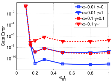
Figure 4: (Color online) $Z$-gate control error vs gating time in a Lorentzian-like environment with $\Omega=\omega_{0}$ and large range control $\left|\epsilon(t)\right|\leq 20\omega_{0}$. The reduced $\alpha/\omega_{0}(t)$ and $\gamma/\omega_{0}(t)$ ratio is responsible for the much smaller gate error. The evolution time scale is shortened (compared to $\omega_{0}^{-1}$), as well as the gating time.

IV Discussion and conclusion

In this work, we show that an exact open non-Markovian qubit dynamics can be readily put in the framework of the QOCT to attain single-qubit gate control. High-fidelity identity gates and $Z$-gates can be achieved for moderate qubit decaying parameters with small magnitude control. The optimal pulses are smooth in shape and easy to implement in experiments. In cases where the open quantum system models are not exactly solvable, the perturbative master equation approaches should be employed for the optimal control solutions JPhysB.40.S75 ; Rebentrost et al. (2009); Wenin and Pötz (2008a); *PhysRevB.78.165118; *wenin:084504; *PhysRevB.79.224516; *PhysRevA.74.022319; Jirari (2009); Gordon et al. (2008); Clausen et al. (2010); Hwang and Goan (2012). However, for models where the exact master equations are available, our present treatment, in contrast to the commonly used perturbation method, is valid for all orders and free from intrinsic error.

The dissipative model and the QOCT method discussed above can be readily applied to realistic physical systems such as the circuit QED system Blais et al. (2004); Wallraff et al. (2004); Circuit_QED_review ; Sarovar05 . In circuit QED, the system is realized by a Josephson charge qubit or a transmon qubit Koch07 coupled to a coplanar waveguide resonator and the qubit frequency can be controlled by external electric voltage and magnetic flux Makhlin et al. (2001); Blais et al. (2004); Koch07 ; Circuit_QED_review . In principle, this formalism can be applied to any two-level system embedded in a structured environment Mazzola et al. (2009), e.g., nitrogen vacancy center in diamond embedded in photonic band-gap Prawer and Greentree (2008).

We introduce the definition of improvement and find that, improvement is directly related to the mathematical nature of $F(t)$. Physically, improvement is in close relation to the shape of the spectral density with respect to the qubit transition frequency. The concept of improvement does not need to be limited to this specific exactly solvable model, but can also be extended to more general systems that allow no exact solutions. Gaining the insight of improvement, one is able to determine in which condition the improvement is notable, and that applying QOCT to the environment-included open system is necessary.

In the model (dissipative model) and the control problem $(\sigma_{z}$ control) discussed in our work, the suppression of dissipation is substantial only when we increase the control strength or, in a physically equivalent sense, enlarge the ratio of the qubit frequency to the qubit-environment coupling strength. This result is in agreement with that implicitly stated in Jing et al. (2013) where nonperturbative dynamical decoupling is applied to the same model.