Dipole amplitude with uncertainty estimate from HERA data and applications in Color Glass Condensate phenomenology
Abstract:
We determine the initial condition for the small- evolution equation (BK) from the HERA deep inelastic scattering data using a new parametrization that also keeps the unintegrated gluon distribution positive. The obtained dipole amplitude and its uncertainty estimate can be used to compute single inclusive particle production in proton-proton and proton-nucleus collisions. We argue that one has to use consistently the proton transverse area measured in DIS and the total inelastic cross section when calculating the single inclusive cross section. This leads to a midrapidity nuclear modification factor that approaches unity at large transverse momentum, independently of the center-of-mass energy.
1 Introduction
The Color Glass Condensate is an effective field theory that provides a convenient framework to describe strongly interacting systems at high energy where non-linear phenomena, such as gluon recombination, become important. These nonlinearities are further increased when the target is changed from a proton to a heavy nucleus, due to the scaling of the gluon densities.
A key ingredient in the CGC calculations is the dipole-proton amplitude, whose evolution in Bjorken- (or equivalently, energy) is given by the the BK equation [1, 2] (with running coupling corrections derived in Ref. [3]). Perturbative techniques can be used to derive the BK equation, but its initial condition, the dipole-proton amplitude at initial , is a non-perturbative input. It can be obtained by performing a fit to proton structure function data measured in deep inelastic scattering (DIS) experiments.
A crucial test for the CGC framework comes from the fits to the combined proton structure function data from the H1 and ZEUS experiments at HERA [4, 5]. A good fit to this precise data can be obtained by using a simple parametrization for the initial dipole amplitude, see Refs. [6, 7].
In this work we discuss how the dipole amplitude is obtained from the HERA DIS data and how the obtained dipole-proton amplitude can be used to describe proton-proton and proton-nucleus collisions. This is reported in more detail in Ref. [6]. We also report ongoing work on the analysis of how tightly the DIS data constrains the initial conditions: we evaluate the uncertainty estimate for the dipole amplitude and study the propagation of these uncertainties to other observables.
2 Fitting the dipole amplitude
The H1 and ZEUS experiments have measured the proton structure functions and , and published the precise combined results for the reduced cross section [4], which is a function of the proton structure functions:
| (1) |
where is the Bjoken-, is the virtuality of the photon and stands for the inelasticity. The structure functions can be computed from the Color Glass Condensate framework by evaluating the virtual photon-proton cross section
| (2) |
where is the photon light cone wave function describing how the photon fluctuates to a quark-antiquark pair, computed from light cone QED [8]. The QCD dynamics is encoded in the dipole-proton amplitude , and the summation is over active quark favours. In this work we do not take into account the heavy quarks, but we note that if the heavy quarks are included one should also include in the analysis the measured charm contribution to from Ref. [5]. We assume that the impact parameter dependence can be factorized and we replace by (twise the proton DIS area) which is a fit parameter.
For the dipole amplitude at we use a modified McLerran-Venugopalan model [9]:
| (3) |
where we have generalized the AAMQS [7] form (labeled as MVγ) by also allowing the constant inside the logarithm, which plays a role of an infrared cutoff, to be different from . The other fit parameters are the anomalous dimension and the initial saturation scale . The last fit parameter is the scale at which the running coupling is evaluated in transverse coordinate space, which we write as and fit . We fit three different initial conditions to the HERA data, and the fit result is shown in Table 1.
The first initial condition used is the standard MV model where . The second parametrization considered here is the MVγ in which is a fit parameter but . The third parametrization is labeled as MVe, and it has but is free. A motivation for the last parametrization is that the Fourier-transform of , which is proportional to the unintegrated gluon distribution, is not positive definite when the MVγ parametrization is used.
3 Dipole amplitude for nuclear targets
We generalize the dipole-proton amplitude to dipole-nucleus scattering by using the optical Glauber model, and write the dipole-nucleus amplitude as
| (4) |
where is the total dipole-proton cross section. In order to satisfy the requirement at large dipoles we use a non-unitarized version of the dipole-proton cross section and obtain (for more details, see Ref. [6])
| (5) |
4 Uncertainty analysis
The experimental uncertainties can be propagated to the fitted dipole amplitude using the Hessian method [10] where one uses a quadratic approximation
| (6) |
Here the best fit parameters, that minimise , are , and the Hessian matrix can be related to the second partial derivatives of with respect to the fit parameters. The eigenvectors of the Hessian matrix serve as an uncorrelated basis for the error sets of the fit parameters . Using the error sets one can, following the procedure used in Ref. [11], compute an uncertainty estimate for any quantity that depends on the dipole amplitude as
| (7) |
In our preliminary analysis we construct very conservatively the error sets such that , the difference of obtained by using the best fit set or the error set , is chosen to be .
5 Single inclusive particle production
The gluon spectrum in heavy ion collisions can be obtained by solving the classical Yang-Mills equations of motion for the color fields. For it has been shown numerically [12] that this solution is well approximated by the following -factorized formula [13]
| (8) |
Here is the dipole unintegrated gluon distribution (UGD) of the proton [14, 15, 16] proportional to the two-dimensional Fourier transform of , where is the dipole amplitude in the adjoint representation. The impact parameter dependece is assumed to factorize. For a detailed expressions, see Ref. [6]. This gives the invariant yield as
| (9) |
where is the two-dimensional Fourier transform of .
Assuming that is much larger than the saturation scale of one of the colliding objects we obtain the hybrid formalism result
| (10) |
where is the integrated gluon distribution function. For it we can use the conventional parton distribution function, and in this work the CTEQ LO [17] pdf is used. Note that the overall normalization factor is obtained by using both the proton area measured in DIS, , and the inelastic proton-proton cross section , consistently in the calculation.
| Model | [GeV2] | [GeV2] | [mb] | ||||
|---|---|---|---|---|---|---|---|
| MV | 2.76 | 0.104 | 0.139 | 1 | 14.5 | 1 | 18.81 |
| MVγ | 1.17 | 0.165 | 0.245 | 1.135 | 6.35 | 1 | 16.45 |
| MVe | 1.15 | 0.060 | 0.238 | 1 | 7.2 | 18.9 | 16.36 |
6 Results
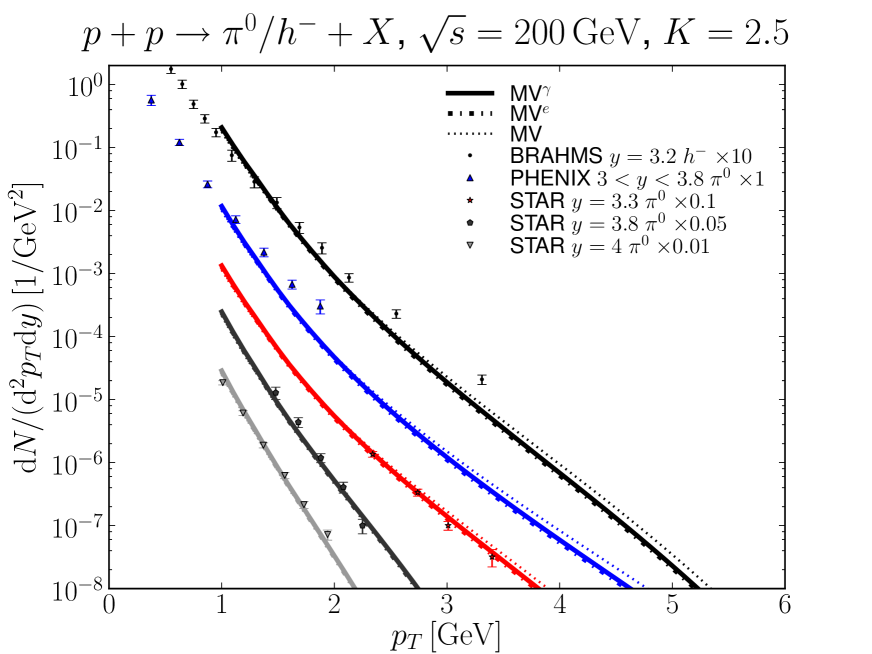
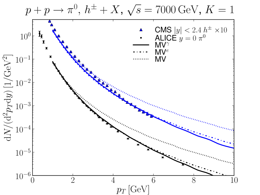
In Fig. 2 we show the single inclusive and negative hadron yields computed using the hybrid formalism and compared with the RHIC data [18, 19, 20]. As the calculation is done at leading order, it is not suprising that overall normalization does not agree with the data, but a normalization factor is needed. As we consider different proton areas consistently when deriving the hybrid formalism result and obtain a correct normalization factor for the LO calculation, the absolute value of the factor quantifies how much the LO result differs from the data. The comparison with the LHC data [21, 22] is shown in Fig. 2. We notice that even though the standard MV model gives relatively good agreement with the data, and especially works well with the RHIC forward data, comparison with the midrapidity LHC measurements clearly rules out the MV parametrization.
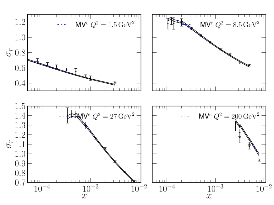
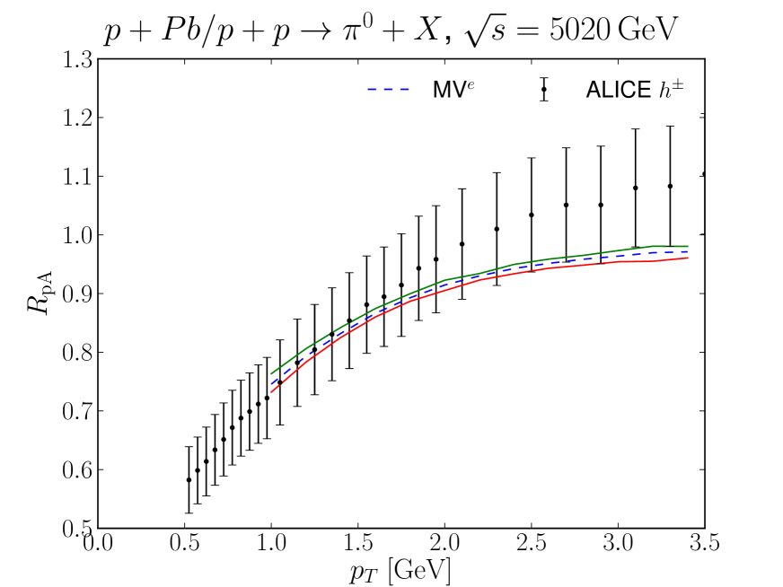
The computed reduced cross section and the uncertainty estimates are compared with the HERA data in Fig. 4. Due to the accuracy of the data the uncertainty band is quite narrow, but the agreement with the data is very good except at largest that is not included in the fit. As a second application we show in Fig. 4 the nuclear suppression factor and compare with the ALICE data [23]. Even tough we have chosen to use very conservative error sets, the effect on is very small. This suggest that is not sensitive to the details of the dipole amplitude, and thus is a solid CGC prediction. We have analytically shown in Ref. [6] that we get midrapidity at all at large which is consistent with the ALICE data.
Acknowledgements
We thank H. Paukkunen for discussions. This work has been supported by the Academy of Finland, projects 133005, 267321, 273464 and by computing resources from CSC – IT Center for Science in Espoo, Finland. H.M. is supported by the Graduate School of Particle and Nuclear Physics.
References
- [1] I. Balitsky, Nucl. Phys. B463, 99 (1996), [arXiv:hep-ph/9509348].
- [2] Y. V. Kovchegov, Phys. Rev. D60, 034008 (1999), [arXiv:hep-ph/9901281 [hep-ph]].
- [3] I. Balitsky, Phys. Rev. D75, 014001 (2007), [arXiv:hep-ph/0609105 [hep-ph]].
- [4] H1 and ZEUS, F. Aaron et al., JHEP 1001, 109 (2010), [arXiv:0911.0884 [hep-ex]].
- [5] H1 and ZEUS, H. Abramowicz et al., Eur. Phys. J. C73, 2311 (2013), [arXiv:1211.1182 [hep-ex]].
- [6] T. Lappi and H. Mäntysaari, Phys. Rev. D88, 114020 (2013), [arXiv:1309.6963 [hep-ph]].
- [7] J. L. Albacete, N. Armesto, J. G. Milhano, P. Quiroga-Arias and C. A. Salgado, Eur. Phys. J. C71, 1705 (2011), [arXiv:1012.4408 [hep-ph]].
- [8] Y. V. Kovchegov and E. Levin, Quantum chromodynamics at high energy (Cambridge University Press, 2012).
- [9] L. D. McLerran and R. Venugopalan, Phys. Rev. D49, 2233 (1994), [arXiv:hep-ph/9309289].
- [10] J. Pumplin et al., Phys. Rev. D65, 014013 (2001), [arXiv:hep-ph/0101032 [hep-ph]].
- [11] K. J. Eskola, H. Paukkunen and C. Salgado, JHEP 0904, 065 (2009), [arXiv:0902.4154 [hep-ph]].
- [12] J. P. Blaizot, T. Lappi and Y. Mehtar-Tani, Nucl. Phys. A846, 63 (2010), [arXiv:1005.0955 [hep-ph]].
- [13] Y. V. Kovchegov and K. Tuchin, Phys. Rev. D65, 074026 (2002), [arXiv:hep-ph/0111362 [hep-ph]].
- [14] D. Kharzeev, Y. V. Kovchegov and K. Tuchin, Phys. Rev. D68, 094013 (2003), [arXiv:hep-ph/0307037 [hep-ph]].
- [15] J. P. Blaizot, F. Gelis and R. Venugopalan, Nucl. Phys. A743, 13 (2004), [arXiv:hep-ph/0402256 [hep-ph]].
- [16] F. Dominguez, C. Marquet, B.-W. Xiao and F. Yuan, Phys. Rev. D83, 105005 (2011), [arXiv:1101.0715 [hep-ph]].
- [17] J. Pumplin et al., JHEP 0207, 012 (2002), [arXiv:hep-ph/0201195 [hep-ph]].
- [18] STAR, J. Adams et al., Phys. Rev. Lett. 97, 152302 (2006), [arXiv:nucl-ex/0602011 [nucl-ex]].
- [19] PHENIX, A. Adare et al., Phys. Rev. Lett. 107, 172301 (2011), [arXiv:1105.5112 [nucl-ex]].
- [20] BRAHMS, I. Arsene et al., Phys. Rev. Lett. 93, 242303 (2004), [arXiv:nucl-ex/0403005 [nucl-ex]].
- [21] ALICE, B. Abelev et al., Phys. Lett. B717, 162 (2012), [arXiv:1205.5724 [hep-ex]].
- [22] CMS, V. Khachatryan et al., Phys. Rev. Lett. 105, 022002 (2010), [arXiv:1005.3299 [hep-ex]].
- [23] ALICE, B. Abelev et al., Phys. Rev. Lett. 110, 082302 (2013), [arXiv:1210.4520 [nucl-ex]].