Abstract

We consider a method of remote mixed state creation of a one-qubit subsystem (receiver) in a spin-1/2 chain governed by the nearest-neighbor $XY$-Hamiltonian. Owing to the evolution of the chain along with the variable local unitary transformation of the one- or two-qubit sender, a large variety of receiver states can be created during some time interval starting with a fixed initial state of the whole quantum system. These states form the creatable region of the receiver’s state-space. It is remarkable that, having the two-qubit sender, a large creatable region may be covered at a properly fixed time instant $t_{0}$ using just the variable local unitary transformation of the sender. In this case we have completely local control of the remote state creation. In general, for a given initial state, there are such receiver’s states that may not be created using the above tool. These states form the unavailable region. In turn, this unavailable region might be the creatable region of another sender. Thus, in future, we have a way to share the whole receiver’s state-space among the creatable regions of several senders. The effectiveness of remote state creation is characterized by the density function of the creatable region.

I Introduction

Remote state creation means the creation of a needed state of some selected subsystem of a quantum system (receiver) using the local operations on another subsystem (sender). First, this problem appeared as a teleportation problem of unknown state from the sender (Alica) to the receiver (Bob) BBCJPW ; BPMEWZ ; BBMHP using pairs of entangled qubits YS1 ; YS2 ; ZZHE . It is important to note that all existing quantum teleportation algorithms use a classical channel of information transfer as a necessary constituent. Decreasing the necessary amount of classically transmitted information is one of the directions of development of remote state preparation algorithms BDSSBW ; BHLSW ; PBGWK2 ; PBGWK ; DLMRKBPVZBW ; XLYG ; G . Regarding experimental realizations of remote state preparation, one should note the experiments with pairs of entangled photons, which are widely used for this purpose ZZHE ; BPMEWZ ; BBMHP ; PBGWK2 ; PBGWK ; DLMRKBPVZBW . The remote preparation of a single-qubit state with all three controllable parameters was studied in refs. PBGWK2 ; XLYG ; PBGWK . Emphasize that an inherent aspect is the entanglement between (some of) the qubits of sender and receiver in (almost) all the above references. In addition, the discord as a resource for remote state preparation was studied, for instance, in DLMRKBPVZBW ; G .

As a special case of the remote state creation, we point out the problem of pure one-qubit quntum state transfer in spin-1/2 chains. This problem was first formulated in the well-known paper by Bose Bose and now it represents a special area of quantum information processing. Several methods of either perfect CDEL ; ACDE ; KS or high-fidelity (probability) KF ; KZ ; GKMT ; FZ state transfer have been proposed and studied. Perhaps the best known systems are the spin chain with properly adjusted coupling constants (the so-called fully engineered spin chain) CDEL ; ACDE ; KS and the homogeneous spin chain with remote end nodes (the so-called boundary-controlled spin chain) GKMT ; WLKGGB .

It was noted that high-fidelity state transfer requires the very rigorous adjustment of the parameters of a chain such as the coupling constants CDEL ; ACDE ; KS and/or the local distribution of external magnetic field DZ . Such a chain is very sensitive to perturbations of its parameters, which lead, in particular, to significant decrease of the state transfer fidelity CRMF ; ZASO ; ZASO2 ; ZASO3 ; SAOZ . Although the boundary-controlled chain is much simpler to realize, the price for this is the long state transfer time, which significantly reduces the effectiveness of such a chain FKZ .

Alternatively, the transfer of complete information about the initial mixed state of a given subsystem (sender) to another subsystem (receiver) was proposed as a development of the state transfer methods Z_2012 (state-information transfer). Information transfer is not sensitive to the parameters of the transfer line Z_2012 . After the information about the sender’s state is obtained by the receiver at some time instant, the initial state of the sender may be recovered (if needed) using the local (non-unitary) transformation, namely, by solving the system of linear algebraic equations.

Note, that the state transfer described in the above quoted references does not explicitly uses the concepts of quantum correlations between the sender and receiver, although they are responsible for that process. The relation between state transfer and entanglement (as a measure of quantum correlations) was studied, for instance, in Bose ; VGIZ ; GKMT ; GMT ; BB ; DFZ ; DZ . In addition, based on the result in Z_2012 concerning information transfer, the so-called informational correlation Z_inf was introduced, showing the sensitivity degree of the receiver’s state to the local unitary transformations of the sender. This measure seems to be more closely related to remote state creation.

The remote state creation algorithm proposed in this paper combines the ideas of both pure state transfer Bose ; CDEL ; ACDE ; KS ; KF ; KZ ; GKMT ; FZ ; WLKGGB and mixed state-information transfer Z_2012 . More precisely, we study the creation problem of possible receiver states at some instant $t$ starting with some initial state of the whole system and using only the initial local unitary transformation $U^{A}$ of the sender. Herewith, the evolution of the whole system is governed by a certain Hamiltonian. This gives us a tool for remote receiver state creation using the parameters of the unitary transformation $U^{A}$ and the time $t$ as control parameters of the state creation process.

We point out that the role of the classical channel of information transfer is the basic difference between our algorithm and the state creation algorithms studied in refs. BDSSBW ; BHLSW ; PBGWK2 ; PBGWK ; DLMRKBPVZBW ; XLYG ; G . Traditionally, the classical channel is used to transmit (part of) the classical information about a quantum state, while we use this channel to transmit only the information about the time instant required to register the needed state. Moreover, in our case, the classical channel is needed only in the simplest cases and may be disregarded in general, as explained in Sec.II and demonstrated with an example of Sec.III.3. In this case, state creation is completely quantum.

For the purpose of remote state creation, we use a particular quantum system, a spin-1/2 chain. At this stage, we do not study the effect of quantum correlations (measured via either the entanglement Wootters ; HW ; P ; AFOV ; HHHH , the discord HV ; OZ ; Zurek , or the informational correlation Z_inf ) on state-creation processes, postponing this aspect for further study.

Hereafter, by the state of a particular subsystem $S$ of a quantum system we mean the reduced density matrix (the marginal matrix)

$$\rho^{S}=Tr_{rest}\rho,$$ (1)

where $\rho$ is the density matrix of the whole system and the trace is calculated with respect to the rest of the quantum system. This means that some additional projection procedure is required to extract the needed state of subsystem $B$. Experimental realization of this projection is not studied here. Of course, state (1) is achievable much more simpler than the product state $\rho=\rho^{rest}\otimes\rho^{B}$, which would be of more interest (the trace in eq.(1) becomes trivial in that case). But the requirement of getting a product state would lead to additional severe relations among the parameters of the sender’s initial state and perhaps would require an increase in the dimensionality of the sender’s Hilbert space. All this would complicate the calculations. Thus, we choose state (1) as a simpler case of remote state creation, allowing us to study a set of features of the state creation process.

Our algorithm relates the particular initial sender’s state with the proper receiver’s state at some time instant. Therefore, the considered process may be viewed as a map (not unique, in general) of the initially prepared sender’s states to the proper receiver’s state. Thus, keeping the term ”state creation”, we specify the state-creation tool, which involves two initially controllable steps: (i) the creation of the selected initial state of the whole system (ii) the implementation of the appropriate local unitary transformation of the sender with the purpose of creating the needed receiver state. Therewith, the parameters of unitary transformation are referred to as the control parameters. After these two initial steps, the receiver’s state is ”built” in an uncontrollable way through the transfer of quantum information about the sender’s state Z_2012 . This transfer is realized owing to the evolution of the whole quantum system governed by a certain Hamiltonian. To emphasize this feature, we call our creation process ”remote state creation through quantum information transfer”.

The problem of remote state creation in a spin-1/2 chain using a sender and a receiver of different dimensionalities $N^{A}$ and $N^{B}$ is a very complicated multi-parametric one. In this paper, after representing some general statements regarding this process, we concentrate on the particular examples of short homogeneous chains with a one-qubit receiver (the end-node of the chain) and a one(two)-qubit sender (the first node(s) of the chain). We consider state creation during a time interval $0\leq t\leq T$ with a fixed $T$ (note that the parameter $T$ appears owing to the periodicity of the evolution of the considered finite system; this parameter depends on the smallest (by absolute value) eigenvalue of the Hamiltonian) and show that, if we use a two-qubit sender ($N^{A}=4>N^{B}=2$), a large variety of receiver states may be created at some properly fixed time instant $t_{0}$, $0\leq t_{0}\leq T$, using just the local unitary transformation $U^{A}$ with variable parameters. This effect is impossible in the case of a one-qubit sender, i.e., when $N^{A}=N^{B}=2$.

We point out the fact that, in general, there are receiver states which can not be created using the above creation tool. These states form the unavailable region in the whole receiver state-space. This is an interesting characteristics of the state creation process. At the first glance, it restricts the capability of the proposed state creation mechanism. However, this property might allow us to divide the whole space of the receiver states into subspaces controllable by different senders. The use of such splitting is evident but we leave the problem of sharing the receiver’s state-space among several senders beyond the scope of this paper.

The paper is organized as follows. General ideas on the state creation as a map of the control parameters of the sender to the required parameters of the receiver are formulated in Sec.II for an arbitrary quantum system governed by a certain Hamiltonian. Mixed state creation in a homogeneous spin-1/2 chain governed by the nearest-neighbor $XY$-Hamiltonian with a one-qubit receiver and one- or two-qubit sender is studied in Sec.III. Basic results are briefly discussed in Sec.IV. Auxiliary information (and calculations) regarding one-qubit pure state transfer, some details on state creation with one- and two-qubit sender, and the basis of the Lie algebra of $SU(4)$ is presented in the Appendix, Sec.V.

II Remote state-creation of a subsystem of a quantum system.

II.1 General state creation algorithm

In this section, we consider general aspects of the remote state creation through the quantum information transfer. To simplify our calculations, we deal with a particular type of the initial states, namely, the states representable by the tensor product of three diagonal blocks:

$$\rho_{0}=\rho^{A}_{0}\otimes\rho^{C}_{0}\otimes\rho^{B}_{0}.$$ (2)

Here $\rho^{A}_{0}$, $\rho^{B}_{0}$ and $\rho^{C}_{0}$ describe the initial states of the sender, receiver and transmission line respectively. Being diagonal, these matrices are composed by the eigenvalues of the initial state. The remote state creation algorithm can be splitted into the following steps.

1. Create the initial state of the sender, receiver and transmission line.

2. Apply the unitary transformation $U(\varphi)$ to the subsystem $A$ to obtain the new initial density matrix $\rho_{0}(\varphi)$:

   $$\rho_{0}(\varphi)=(U^{A}(\varphi)\rho^{A}_{0}(U^{A}(\varphi))^{+})\otimes\rho^{C}_{0}\otimes\rho^{B}_{0},$$ (3)

   where $\varphi=\{\varphi_{1},\dots,\varphi_{(N^{A})^{2}-1}\}$ is the list of parameters of the unitary transformation $U^{A}\in SU(N^{A})$ which may vary in an arbitrary way. However, not all $(N^{A})^{2}-1$ parameters of this transformation may affect the receiver’s state (as is demonstrated below in this section) and, in principle, some additional constraints may be imposed on these parameters. The choice of parameters $\varphi_{i}$ is predicted by the needed receiver’s state.

3. Switch on the quantum evolution governed by a certain Hamiltonian $H$ in accordance with the Liouville equation

   $$\rho(\varphi,t)=e^{-it{{H}}}\rho_{0}(\varphi)e^{it{{H}}}.$$ (4)

   The information about the initial sender’s state transfers to the receiver on this step.

4. Finally, the state of the subsystem $B$ at the time instant $t$ is described by the marginal matrix $\rho^{B}(\varphi,t)$,

   $$\rho^{B}(\varphi,t)={\mbox{Tr}}_{A,C}\rho(\varphi,t).$$ (5)

   As pointed out in the Introduction, Sec.I, formula (5) means that the final state of the whole system, in general, is not a product state, i.e., $\rho(\varphi,t)\neq\rho^{AC}(\varphi,t)\otimes\rho^{B}(\varphi,t)$. Thus, in the real experiment, an additional projection procedure is needed to extract this state.

We see that the first and the second steps of this algorithm are controllable. Both these steps serve to create the initial state of the whole system. The principal differences between them are following.

1. The first step is ”non-local” because it involves all three subsystems. On the contrary, the second step is local, it modifies the sender’s initial state created on the first step.

2. The first step deals with the eigenvalues of all three subsystems, while the second step does not affect any eigenvalue.

3. The local parameters $\varphi_{i}$ may vary depending on the required receiver’s state. In other words, they are the control parameters, unlike the eigenvalues remaining unchanged during the state creation process.

From the above discussion it follows that the parameters of the local unitary transformation $U^{A}$ provide the tool allowing us to control the remote state creation process. This control tool is characterized in next Sec.II.2.

II.2 State creation with pure sender’s initial state

First of all, we shall note that not all $(N^{A})^{2}-1$ parameters of the local unitary transformation $U^{A}\in~{}SU(N^{A})$ can affect the state of receiver. We consider the map between the sender’s control parameters and the receiver’s creatable parameters in the case of pure sender’s initial state and deduce the number of effective control parameters of $U^{A}$ (i.e., parameters which may really affect the receiver’s state) as a function of the sender dimensionality $N^{A}$.

It was shown TBS ; Z_QIP that $N^{A}-1$ parameters $\varphi_{i}$ (the number of independent eigenvalues) disappear from initial state (3) because of the diagonality of the initial density matrix $\rho^{A}_{0}$. In addition, the sender’s initial density matrix $\rho^{A}_{0}$ has a single non-zero eigenvalue (the pure state), so that the number of variable parameters of $U^{A}$ decreases by $(N^{A}-1)(N^{A}-2)$ owing to the additional symmetry with respect to the transformation ${\mbox{diag}}\{1,\tilde{U}\}$, $\tilde{U}\in SU(N^{A}-1)$. Thus, we stay with

$$D^{A}=(N^{A})^{2}-1-(N^{A}-1)-(N^{A}-1)(N^{A}-2)=2(N^{A}-1)$$ (6)

parameters $\{\varphi_{1},\dots,\varphi_{2(N^{A}-1)}\}$.

Now we consider evolution (4) governed by a certain Hamiltonian $H$. Consequently, the time $t$ appears as one more variable parameter. Thus, we have $D^{A}+1=2(N^{A}-1)+1$ variable real parameters of the sender which we refer to as the control parameters of the state creation algorithm.

In turn, the receiver’s state of general position (5) contains $(N^{B})^{2}-1$ parameters which we refer to as the creatable parameters of the state creation algorithm. Therewith $N^{B}-1$ creatable parameters represent the independent eigenvalues $\lambda_{i}$ ($i=1,\dots,N^{B}-1$) of $\rho^{B}$, while the rest $N^{B}(N^{B}-1)$ parameters $\beta_{i}$ appear in the eigenvector matrix $U(\beta)$ of $\rho^{B}$, where all the parameters $\beta_{i}$ are collected in the list $\beta=\{\beta_{1},\dots,\beta_{N^{B}(N^{B}-1)}\}$. Thus, the density matrix of the receiver’s state may be written as

$$\rho^{B}=U(\beta)\Lambda U^{+}(\beta),\;\;\;\Lambda={\mbox{diag}}(\lambda_{1},\dots,\lambda_{N^{B}}),\;\;\;\sum_{i=1}^{N^{B}}\lambda_{i}=1.$$ (7)

As a result, we have the following map of $D^{A}+1$ control parameters of the sender’s state into $D^{B}$ creatable parameters of the receiver’s state:

$${\mathcal{M}}(\varphi,t;\lambda,\beta):\;\{\varphi_{1},\dots,\varphi_{2(N^{A}-1)},t\}\to\{\lambda_{1},\dots,\lambda_{N^{B}-1},\beta_{1},\dots,\beta_{N^{B}(N^{B}-1)}\}.$$ (8)

We see that the number of variable parameters increases linearly with $N^{A}$ in the case of pure sender’s initial state.

In principle, since we consider a finite quantum system, all the creatable parameters $\lambda_{i}$ and $\beta_{i}$ may be analytically expressed in terms of the control parameters $\varphi_{i}$ and $t$. However, these expressions are very combersome even for small systems, so that the numerical consideration is a proper way of dealing with map (8).

Obviously, we may hope to create the whole receiver’s state-space if

$${\mbox{the number of control parameters }}\;\;\geq\;\;{\mbox{the number of creatable parameters }},$$ (9)

or, regarding map (8),

$$2(N^{A}-1)+1\geq(N^{B})^{2}-1.$$ (10)

If inequality in (9) is strong (i.e., relation ”$>$” is realized), then the time may be disregarded as a control parameter without destroying the validity of (9). Consequently, we may expect to create the whole (or large) region of the receiver’s state-space at a (properly) fixed time instant $t_{0}$ (the time instant $t_{0}$ is determined by the periodic behavior of the considered finite quantum system and will be found in Sec.III.3 (see also Sec.V.3) for a particular example). Disregarding the time $t$ in map (8), we reduce this map to the following one:

$${\mathcal{M}}(\varphi;\lambda,\beta):\;\{\varphi_{1},\dots,\varphi_{2(N^{A}-1)}\}\to\{\lambda_{1},\dots,\lambda_{N^{B}-1},\beta_{1},\dots,\beta_{N^{B}(N^{B}-1)}\}.$$ (11)

We shall note, that the only difference between maps (8) and (11) is the time $t$ in the list of control parameters of map (8). However, because of this additional parameter, map (8) may not be considered as a completely local one. In fact, to obtain the required state of receiver, one has to transfer the information about the proper time instant of the state registration (classical channel). On the contrary, map (11) is completely local because the receiver registers the state at a fixed time instant $t_{0}$, which can be reported in advance. Note that the classical channel mentioned above transmits the information about the registration time instant rather then the information about the state itself as in the other state-creation algorithms BDSSBW ; BHLSW ; PBGWK2 ; PBGWK ; DLMRKBPVZBW ; XLYG ; G .

Below, in Sec.III, we consider the pure initial state of sender. This choice is cased by the conclusion following from the numerical experiments with different initial states $\rho^{A}(0)$. Namely, the maximal region of creatable states (or the creatable region) is associated with the pure sender’s initial state.

Apparently, the classical perfect pure one-qubit state transfer along the spin chain Bose may be considered as a very special case of the remote state creation process, see Appendix V.1.

III Examples of state creation in short homogeneous spin-1/2 chains

III.1 Homogeneous spin-1/2 chain governed by nearest-neighbor XY Hamiltonian

Let us consider the open spin-1/2 chain with the one-qubit receiver $B$ and the one- or two-qubit sender $A$. For definiteness, let $A$ and $B$ be placed, respectively, in the beginning and in the end of this chain. Therewith, the rest nodes of spin chain form the subsystem $C$ which we call the transmission line. Thus, we have a three-partite quantum system $A-C-B$. For simplicity, only the one-qubit transmission line $C$ is considered here. Of course, such a transmission line is a very short one, but, nevertheless, it enriches the features of the state-creation process. We assume that the spin dynamics is governed by the nearest-neighbor $XY$ Hamiltonian $H$,

$${{H}}=-\sum_{j=1}^{3}\frac{d}{2}(I^{+}_{j}I^{-}_{j+1}+I^{-}_{j}I^{+}_{j+1}).$$ (12)

Here $d$ is the coupling constant between the nearest neighbors, $I^{\pm}_{j}=I_{x;j}\pm iI_{y;j}$, $I_{\alpha;j}$, $\alpha=x,y,z$, are the projection operators of the $i$th spin angular momentum. We put $d=1$ without the loss of generality.

Below we consider the state-creation with the one- and two-qubit senders in more details.

III.2 Three-node chain with one-qubit sender

We proceed with the three node chain having the one-qubit subsystems $A$ (the 1st node), $B$ (the 3rd node) and $C$ (the 2nd node), thus $N^{A}=N^{B}=2$. We consider a pure initial states of the subsystems $A$ and $C$ and a mixed initial state of the receiver $B$. Thus, the initial state of the whole spin chain is given by expression (2) with

$$\rho^{A}_{0}={\mbox{diag}}(1,0),\;\;\rho^{C}={\mbox{diag}}(1,0),\;\;\rho^{B}={\mbox{diag}}(\lambda^{B},1-\lambda^{B}).$$ (13)

The unitary $SU(2)$ transformation $U^{A}$ responsible for the state creation is the two-parametric one:

$$U^{A}(\varphi) = e^{-i\pi\varphi_{2}\sigma_{3}}e^{-i\frac{\pi\varphi_{1}}{2}\sigma_{2}}e^{i\pi\varphi_{2}\sigma_{3}}=\left(\begin{array}[]{cc}\cos\frac{\pi\varphi_{1}}{2}&-e^{-i2\pi\varphi_{2}}\sin\frac{\pi\varphi_{1}}{2}\cr e^{i2\pi\varphi_{2}}\sin\frac{\pi\varphi_{1}}{2}&\cos\frac{\pi\varphi_{1}}{2}\end{array},\right)$$ (17)

$$0<\varphi_{i}<1,\;\;i=1,2,\;\;\varphi=\{\varphi_{1},\varphi_{2}\}.$$

The evolution of this chain is described by formula (4) with Hamiltonian (12) in accordance with the Liouville equation. Finally, the state of the subsystem $B$ at some instant $t$ is described by the marginal matrix $\rho^{B}(t)$ (5),

$$\rho^{B}(t)=Tr_{A,C}\rho(t)=Tr_{A,C}e^{-itH}\left(U^{A}\rho^{A}_{0}(U^{A})^{+}\otimes\rho^{C}_{0}\otimes\rho^{B}_{0}\right)e^{itH},$$ (18)

which can be represented in form (7) with

$$\Lambda = {\mbox{diag}}(\lambda,1-\lambda),$$ (19)

$$U = e^{-i\pi\beta_{2}\sigma_{3}}e^{-i\frac{\pi\beta_{1}}{2}\sigma_{2}}e^{i\pi\beta_{2}\sigma_{3}}=\left(\begin{array}[]{cc}\cos\frac{\pi\beta_{1}}{2}&-e^{-i2\pi\beta_{2}}\sin\frac{\pi\beta_{1}}{2}\cr e^{i2\pi\beta_{2}}\sin\frac{\pi\beta_{1}}{2}&\cos\frac{\pi\beta_{1}}{2}\end{array}\right),$$

$$0<\beta_{i}<1,\;\;i=1,2,\;\;\beta=\{\beta_{1},\beta_{2}\},\;\;\frac{1}{2}\leq\lambda\leq 1.$$

Here the parameters $\beta_{i}$, $i=1,2$, and $\lambda$ depend on $\varphi$ and $t$, but we do not write them as arguments for the brevity. Now transformation (8) reads

$${\mathcal{M}}(\varphi,t;\lambda,\beta):\;\{\varphi_{1},\varphi_{2},t\}\to\{\lambda,\beta_{1},\beta_{2}\},$$ (25)

$$0\leq\varphi_{i}\leq 1,\;\;i=1,2,\;\;0\leq t\leq\pi\sqrt{2},$$

$$0\leq\beta_{i}\leq 1,\;\;i=1,2,\;\;1/2\leq\lambda\leq 1.$$

It is remarkable that map (25) admits a simplification due to the linear relation between the parameters $\varphi_{2}$ and $\beta_{2}$ (see Appendix V.2), i.e., the transformation $\varphi_{2}\to\beta_{2}$ becomes trivial. This allows us to disregard the parameters $\varphi_{2}$ and $\beta_{2}$ in map (25-25) and replace this map with the following one:

$${\mathcal{M}}(\varphi_{1},t;\lambda,\beta_{1}):\;\{\varphi_{1},t\}\to\{\lambda,\beta_{1}\},$$ (26)

$$0\leq\varphi_{1}\leq 1,\;\;0\leq t\leq\pi\sqrt{2},$$ (27)

$$0\leq\beta_{1}\leq 1,\;\;1/2\leq\lambda\leq 1,$$ (28)

where we consider $\lambda\geq 1/2$ without the loss of generality. No new states may be created at $t>\pi\sqrt{2}$, which follows from the periodicity of the spin-dynamics and is justified by the numerical simulations. Map (26-28) is numerically studied in the following subsection.

III.2.1 Numerical study of state creation with one-qubit sender

We consider map (26-28) with initial condition (13). The creatable region in the space $(\lambda,\beta_{1})$ (28) is depicted in Fig.1a-d for the following set of $\lambda^{B}$:

$$\lambda^{B}=1,\;\;\frac{3}{4},\;\;\frac{1}{4},\;\;0.$$ (29)

Therewith, we use the following uniform splitting of the variation intervals of the control parameters

variation interval $$[0,1] \varphi_{1}$$ of is splitted into 399 segments (400 points) (30)

$${\mbox{variation interval $[0,\pi\sqrt{2}]$ of $t$ is splitted into 2399 segments (2400 points)}}.$$

Each point on this figure corresponds to a particular receiver’s state. We see that these points form smooth lines and each of these lines corresponds to a particular time instant of map (26) with the parameter $\varphi_{1}$ running the interval $[0,1]$ specified in (27). In the case of pure initial state, $\lambda^{B}=1,0$, the lines cover the whole space $(\lambda,\beta_{1})$ (see Fig.1a,d). The vertical lines $\lambda=1$ in these figures are associated with the time instant $t=\pi\sqrt{2}$ corresponding to the perfect one-qubit pure state transfer from the first to the third node CDEL . The case of the initial state with $\lambda^{B}=1$ (Fig.1a) is of the most interest because the map (26) is mutually unique. Moreover, the lines are time-ordered in this case: the time instant prescribed to each of these lines increases in the direction of the arrows from $0$ to $\pi\sqrt{2}$ (the dashed line with arrows is not associated with the receiver’s states). So, in principle, we may construct the one-to-one relation between the pairs ($\varphi_{1}$, $t$) and ($\lambda$, $\beta_{1}$). Thus, having a particular pair ($\lambda$, $\beta_{1}$), we may restore the parameter of sender $\varphi_{1}$ and the time instant $t$ when the state was sent. Fig.1 is aimed to show the overall picture of the receiver’s state distribution. Notice that the ”dense” areas mean that more points from the sender’s state-space are mapped into these areas.

Regarding the mixed initial states $\lambda^{B}=3/4,1/4$, see Fig.1b,c, not any state of the receiver may be created by the local unitary transformations $U^{A}$, which is indicated by the unavailable regions in these figures. In addition, the map (26) is not mutually unique (unlike the case $\lambda^{B}=1$, see Fig.1a) since some particular states ($\lambda$, $\beta_{1}$) can be created by more then one pair ($\varphi_{1}$, $t$) (because some lines cross each other).

We shall also note the case $\lambda^{B}=\frac{1}{2}$ when only the states with $\frac{1}{2}\leq\lambda\leq 1$ and $\beta_{1}=0,1$ (i.e., arbitrary diagonal states) are creatable.

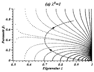
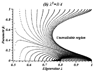
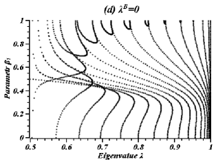
Figure 1: The two-parameter receiver state-space $(\lambda,\beta_{1})$ of map (26-28) for the three node spin chain with the one-qubit sender and set (29) of $\lambda^{B}$ is considered. This figure demonstrates the non-uniform distribution of the creatable states. (a) $\lambda^{B}=1$, the pure initial state; the whole space $(\lambda,\beta_{1})$ is creatable and map (26) is mutually unique; the time $t$ increases in the direction of the arrows. (b,c) $\lambda^{B}=3/4$ and $\lambda^{B}=1/4$ respectively; the mixed initial state, map (26) is not mutually unique and the unavailable region appears. (d) $\lambda^{B}=0$, the pure initial state; the whole space $(\lambda,\beta_{1})$ is creatable, but map (26) is not mutually unique.

The overall disadvantage of the proposed algorithm of the state creation with equal dimensionalities of the sender and receiver is that we have to involve the time $t$ as a control parameter of map (26) in order to cover a valuable region of the space $(\lambda,\beta_{1})$. Consequently, this map is not completely governed by the local unitary transformation $U^{A}$. This disadvantage is compensated in the case $N^{A}=4$ considered in the next subsection. Notice that the map (26) with a pure initial state covers the complete state-space $(\lambda,\beta_{1})$ only in the case of two and three node chains with the nearest neighbor interactions. Involving the dipole-dipole interaction among all nodes, the unavailable region appears even in the case of three nodes and pure initial state. Besides, the unavailable region appears in the case of longer chains with nearest neighbor interactions as well. In this regard, we have to remember the similar feature of the perfect one-qubit pure state transfer. Namely, the perfect one-qubit pure state transfer is possible along the homogeneous spin-1/2 chains of two and three nodes governed by the nearest neighbor XY Hamiltonian CDEL , and this phenomenon is destroyed by involving all node interactions; the perfect state transfer is also impossible in longer homogeneous chains with nearest neighbor interactions. Thus, the remote creation of the whole state-space and perfect pure state transfer may be organized in the same chain, i.e., in the three-node homogeneous chain governed by the nearest neighbor $XY$ Hamiltonian. However, it is not clear whether this is always valid. The remote state creation using the long non-homogeneous chain with the interaction constants providing the perfect one-qubit pure state transfer between the first and the last nodes CDEL ; KS is not studied here.

III.2.2 Density function as a characteristics of creatable region

The distribution of creatable states in the parameter space $(\lambda,\beta_{1})$ is non-uniform, see Fig.1a-b. This is reflected in the varying density of points in this figure. If we fix some small area in space $(\lambda,\beta_{1})$, then the more points are in this area, the more points from the space $(\varphi_{1},t$) are mapped into it. To better visualize this effect, we introduce the so-called density function as follows:

$$S(\lambda_{i},\beta_{1j})=\lim_{N_{\lambda},N_{\beta_{1}}\to\infty}\frac{s(\lambda_{i},\beta_{1j})}{\varepsilon_{\lambda}\varepsilon_{\beta_{1}}N^{st}},$$ (31)

$$\lambda_{i}=\frac{1}{2}+\varepsilon_{\lambda}i,\;\;i=0,\dots,N_{\lambda}-1,\;\;\beta_{1j}=\varepsilon_{\beta_{1}}j,\;\;j=0,\dots,N_{\beta_{1}}-1,\;\;\varepsilon_{\lambda}=\frac{1}{2N_{\lambda}},\;\;\varepsilon_{\beta_{1}}=\frac{1}{N_{\beta_{1}}},$$

where $s(\lambda_{i},\beta_{1j})$ is the number of states in the rectangle

$$(\lambda_{i},\lambda_{i}+\varepsilon_{\lambda}],\;\;(\beta_{j},\beta_{j}+\varepsilon_{\beta}],$$ (32)

$N^{st}$ is the total number of states in the rectangle (28). The function $S$ is normalized as follows:

$$\sum_{i=0}^{N_{\lambda}-1}\sum_{j=0}^{N_{\beta_{1}}-1}S(\lambda_{i},\beta_{1j})\varepsilon_{\lambda}\varepsilon_{\beta_{1}}=1.$$ (33)

We represent the contour plot of the density function (31) in Fig.2 for $\varepsilon_{\beta_{1}}=2\varepsilon_{\lambda}=\varepsilon=0.01$ and $N^{st}=960000$. This value of $N^{st}$ corresponds to the uniform splitting (30) of the variation intervals (27) of the parameters $\varphi_{1}$ and $t$. Figs.2a-d show the dependence of the density function on $\lambda^{B}$. The choice of $\lambda^{B}$ must be defined by a particular area of states which we need to create. Perhaps, the bright areas are of most interest. The maximal values $S_{max}$ of the density function together with their coordinates $\lambda_{max}$ and $\beta_{1;max}$ for different values of $\lambda^{B}$ from list (29) are collected in Table 1.

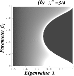
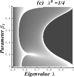
Figure 2: The density function of the two-parameter receiver state-space $(\lambda,\beta_{1})$ of map (26-28) for the three node chain with the one-qubit sender and set (29) of $\lambda^{B}$ is considered ( compare with Fig.1). The bright areas are most ”populated”. The maximal values of the density function $S_{max}$ together with the appropriate values of the parameters $\lambda_{max}$ and $\beta_{1;max}$ are collected in Table 1. (a, d) $\lambda^{B}=1$ and $0$ respectively, the pure initial state; the whole receiver’s state-space may be created. (b, c) $\lambda^{B}=3/4$ and $1/4$ respectively, the mixed initial state; the whole receiver’s state-space may not be created; the unavailable regions are indicated by the black areas in both figures.

$\lambda^{B}$	$1$	$\displaystyle\frac{3}{4}$	$\displaystyle\frac{1}{4}$	$0$
$S_{max}$	3312.29	1283.35	733.92	639.63
$\lambda_{max}$	0.9975	0.7525	0.7475	0.9975
$\beta_{1;max}$	0.005	0.005	0.995	0.995

Table 1: The maximal values $S_{max}(\lambda_{max},\beta_{1;max})$ of the density function of creatable states for the case of one-qubit sender (the three node chain). Remark: One can show that the values $S_{max}$ increase with decrease of $\varepsilon$ in accordance with definition of the density function (31), whereas the coordinates $\lambda_{max}$ and $\beta_{1;max}$ remain unchanged up to the accuracy, respectively, $\pm\varepsilon/2$ and $\pm\varepsilon$. Thus, the values in the 1st line are underestimated. The same remark holds for Table 2.

Although the density function $S$ illustrates the distribution of the creatable states, this distribution is also understandable from Fig.1 because the creatable states are arranged in lines. The case of two-qubit sender (studied in Sec. III.3) is different. The creatable states are not arranged in the well-structured lines, so that the density function $S$ becomes very important in that case.

III.3 Four-node spin chain with two-qubit sender

Let us consider the four node chain with the two-qubit sender (the first and the second nodes), while the receiver (the 4th node) and the transmission line (the 3rd node) remain one-qubit subsystems. As was shown in TBS ; Z_QIP (see also the beginning of Sec.II.2), the local unitary transformation $U^{A}\in SU(4)$ has 12 control parameters in the case of diagonal sender’s initial state $\rho^{A}_{0}$:

$$U^{A}(\varphi)=$$ (34)

$$e^{i\pi\gamma_{3}\varphi_{1}}e^{i\gamma_{2}\frac{\pi\varphi_{2}}{2}}e^{i\pi\gamma_{3}\varphi_{3}}e^{i\gamma_{5}\frac{\pi\varphi_{4}}{2}}e^{i\pi\gamma_{3}\varphi_{5}}e^{i\gamma_{10}\frac{\pi\varphi_{6}}{2}}e^{i\pi\gamma_{3}\varphi_{7}}e^{i\gamma_{2}\frac{\pi\varphi_{8}}{2}}e^{i\pi\gamma_{3}\varphi_{9}}e^{i\gamma_{5}\frac{\pi\varphi_{10}}{2}}e^{i\pi\gamma_{3}\varphi_{11}}e^{i\gamma_{2}\frac{\pi\varphi_{12}}{2}},$$

$$\varphi=\{\varphi_{1},\dots,\varphi_{12}\},\;\;0\leq\varphi_{i}\leq 1,\;\;i=1,\dots,12.$$ (35)

The explicit matrix representation of $\gamma_{i}$ is given in Appendix V.3 TBS ; GM .

We consider the diagonal initial density matrix of form (2) and fix the pure initial state of the subsystems $A$ and $C$, while the initial state of the receiver $B$ is arbitrary diagonal one, similar to Sec.III.2. In other words, our initial matrices are following:

$$\rho_{0}^{A}={\mbox{diag}}(1,0,0,0),\;\;\rho_{0}^{C}={\mbox{diag}}(1,0),\;\;\rho_{0}^{B}={\mbox{diag}}(\lambda^{B},1-\lambda^{B}).$$ (36)

The density matrix evolves in accordance with eq.(4). Finally, the marginal matrix $\rho^{B}(t)$ describing the receiver’s state may be calculated using formulas (18,19) of Sec.III.2, where the Hamiltonian $H$ is the same (see eq. (12)), while $U^{A}$ and $\rho^{A,B,C}_{0}$ are given by eqs.(34) and (36), respectively.

In accordance with Sec.II, in this case, we may disregard the time as a varying parameter of the state creation and use map (11) which now has 6 effective arbitrary parameters in accordance with eq.(6). However, since we need to create the three parametric receiver’s state, it might be enough to take just three parameters $\varphi_{i}$ in the map (11). But these three parameters may not be chosen in an arbitrary way and, in general, the choice of parameters affects the creatable region. The preferable choice of three parameters is not evident, and the problem of the optimal (i.e., leading to the maximal possible creatable region) parametrization of the considered map remains beyond the scope of this paper. Instead, we propose the following parametrization which yields large (and, perhaps, the maximal possible creatable region for the given initial state (36)). At least, the numerical experiments with a set of other parameterizations give the same result, see also Appendix V.4.

In our parametrization, the parameters $\varphi_{10}$, $\varphi_{11}$ and $\varphi_{12}$ vary independently, while all other parameters are linearly expressed in terms of the single parameter $\phi$:

$$\varphi_{2n-1}=\phi,\;\;n=1,\dots,5,$$ (37)

$$\varphi_{2n}=\frac{\phi}{2},\;\;n=1,\dots,4.$$

Thus, the map (11) simplifies to

$${\mathcal{M}}(\varphi,\beta) : \{\varphi_{10},\varphi_{11},\varphi_{12},\phi\}\to\{\lambda,\beta_{1},\beta_{2}\},$$ (40)

$$0\leq\varphi_{i}\leq 1,\;\;i=10,11,12,\;\;0\leq\phi\leq 1,$$

$$0\leq\beta_{i}\leq 1,\;\;i=1,2,\;\;\frac{1}{2}\leq\lambda\leq 1,$$

which is numerically studied in the following subsection. Therewith, we fix a time instant $t_{0}$ inside of some interval,

$$0<t_{0}\leq T,$$ (41)

where the parameter $T$ is related with the periodicity of quantum dynamics of the considered finite spin system. It is closely related with the minimal (in magnitude) eigenvalue $\lambda^{abs}_{min}$: $T\approx\frac{\pi}{\lambda^{abs}_{min}}$ (half of the oscillation period of the real and imaginary parts of the exponent $e^{i\lambda^{abs}_{min}t}$). We have $\lambda^{abs}_{min}\approx 0.309$, so that $T\approx 10.2$. One can show that during this time interval the evolution of the area of creatable region passes through its maximal value

III.3.1 Numerical study of state creation with two-qubit sender

The numerical simulation show that the distribution of the receiver’s states is uniform in $\beta_{2}$, similarly to Sec.III.2 (see Appendix V.4 for details). Perhaps, this means that there is a linear relation between $\beta_{2}$ and a particular parameter of $U^{A}$, similar to the relation between the parameters $\beta_{2}$ and $\varphi_{2}$ in Sec.III.2. However, we do not establish such a relation. We only remove $\beta_{2}$ from the right side of map (40) and study the two-parameter state-space $(\lambda,\beta_{1})$ of the receiver:

$${\mathcal{M}}(\varphi,\beta) : \{\varphi_{10},\varphi_{11},\varphi_{12},\phi\}\to\{\lambda,\beta_{1}\}.$$ (42)

As explained in the Appendix, see the end of Sec.V.4, we choose the time instant $t_{0}=6.4$ inside of interval (41) and perform a set of state-creating experiments substituting different values of $\lambda^{B}$ from set (29) into initial condition (36). Therewith we use the following uniform splitting of the variation intervals $[0,1]$ of the parameters:

$${\mbox{variation intervals of }}\;\;\varphi_{10,12}\;\;\;{\mbox{are splitted into 50 segments (51 points)}},$$ (43)

$${\mbox{variation intervals of }}\;\;\varphi_{11},\phi\;\;\;{\mbox{are splitted into 25 segments (26 points)}}.$$

In all these cases, there is a boundary in the space $(\lambda,\beta_{1})$ separating the creatable and unavailable regions, see also Fig.5a,c in Appendix V.4. Perhaps, both the presence of the unavailable regions for all $\lambda^{B}$ and the fact that the perfect pure state transfer is impossible along the homogeneous four node spin chain governed by the nearest-neighbor XY Hamiltonian CDEL have the same origin.

To simplify the representation of obtained results, we show only the boundaries corresponding to the different values of $\lambda^{B}$ instead of the creatable regions themselves and depicture all these boundaries in the same figure, see Fig.3a. Herewith the creatable region is to the left from the appropriate boundary line, while the unavailable region is to the right from it.

We see that the largest creatable region corresponds to the pure initial states ($\lambda^{B}=1,0$). It is important that there is a small region which may not be created in the chain with initial state (36) and any choice of $\lambda^{B}$ at the selected time instant $t_{0}$. This absolutely unavailable region is indicated in Fig.3a and it is shown in Fig.3b using the proper scale. However, perhaps this region is creatable using another initial state and/or different time instant $t_{0}$. It is interesting to note that the numerically obtained boundaries in Fig.3b can be approximated by the following analytical curves:

$$0.9914-2.0034(0.9999-x)^{0.28} {\mbox{the upper curve}},$$ (44)

$$-0.0100+2.0369(1-x)^{0.28} {\mbox{the lower curve}}.$$

Similar to Sec.III.2.1, the case $\lambda^{B}=\frac{1}{2}$ allows us to create only the arbitrary diagonal states of the receiver, i.e., $\frac{1}{2}\leq\lambda\leq 1$ and $\beta_{1}=0,1$.

,

Figure 3: The two-parameter space $(\lambda,\beta_{1})$ of map (40-40) for the four node chain with the two-qubit sender and set (29) of $\lambda^{B}$ is considered at $t_{0}=6.4$. We represent the boundary curves separating the creatable and unavailable regions of the receiver’s state-space. The creatable region is to the left from the appropriate boundary curve. There is a region which may not be created by any local unitary transformation of the subsystem $A$ with any value of $\lambda^{B}$ (the absolutely unavailable region). The vertical stripe of states with $\frac{1}{2}\leq\lambda\leq 0.52$ is hardly creatable, see also Figs.4 and 5. ($a$) The creatable and unavailable regions of the receiver’s state-space for $\lambda^{B}=1,3/4,1/4,0$. ($b$) The absolutely unavailable region is bounded by the boundaries corresponding to the pure initial states $\lambda^{B}=1$, $0$; the solid lines represent analytical curves (44).

III.3.2 Density function of creatable region

To characterize the effectiveness of the state creation, we use the density function $S(\lambda,\beta_{1})$ introduced in Sec.III.2.2. Herewith, for each $\lambda^{B}$ from set (29), we construct the family of all creatable states varying the parameters of the local transformation $U^{A}$ inside of the region (40). We represent the contour plot of the density function in Fig.4 for $\varepsilon_{\beta_{1}}=2\varepsilon_{\lambda}=\varepsilon=0.01$ and $N^{st}=1758276$. This value of $N^{st}$ is related with uniform splitting (43) of variation intervals (40) of the parameters $\varphi_{10,12}$ and $\varphi_{11}$, $\phi$. The creatable region is maximal for the pure initial states ($\lambda^{B}=1,0$), as is shown in Figs.2a,d. The maximal values $S_{max}$ of the density function together with their coordinates $\lambda_{max}$ and $\beta_{1;max}$ for different $\lambda^{B}$ from set (29) are collected in Table 2.

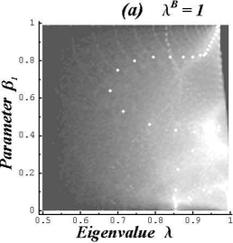
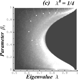
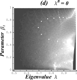
Figure 4: The density function of the two-parameter receiver state-space $(\lambda,\beta_{1})$ of map (40-40) for the four node chain with the two-qubit sender and set (29) of $\lambda^{B}$ is considered. The bright areas to the left from the right boundaries of the creatable regions are most ”populated”. The maximal values of the density function $S_{max}$ together with the appropriate values of the parameters $\lambda_{max}$ and $\beta_{1;max}$ are collected in Table 2. The family of bright spots embedded into the dark areas appears for all $\lambda^{B}$. (a, d) $\lambda^{B}=1$ and $0$ respectively, the pure initial state; unlike the chain with the one-qubit sender, the unavailable region (the black area) appears even in this case. (b, c) $\lambda^{B}=3/4$ and $1/4$ respectively, the mixed initial state; the unavailable regions are indicated by the black areas, these regions are similar to those shown in Figs. 2b,c.

$\lambda^{B}$	$1$	$\displaystyle\frac{3}{4}$	$\displaystyle\frac{1}{4}$	$0$
$S_{max}$	36.96	45.36	43.36	35.28
$\lambda_{max}$	0.8525	0.8475	0.8275	0.9975
$\beta_{1;max}$	0.065	0.025	0.035	0.995

Table 2: The maximal values $S_{max}(\lambda_{max},\beta_{1;max})$ of the density function of creatable states for the case of two-qubit sender (the four node chain)

The unavailable regions (the black right sides) and the hardly creatable regions (the dark left sides) are well depicted in these figures. The most ”populated” areas correspond to the bright parts of the figures. We shall point out the set of bright spots inside of the dark area in each of figures (a)-(d). Perhaps, with increase of $N^{st}$, these spots join with each other forming a smooth line. The position of these sports depends on a particular choice of the parameters $\varphi_{i}$ in map (11) realizing the state creation (like the parameters $\varphi_{i}$, $i=10,11,12$, and $\phi$ in map (40-40)). The meaning and application of these spots are not clear.

IV Conclusions and discussion

We study the problem of remote creation of the mixed receiver’s states using the variable local unitary transformations of the sender and assuming that the receiver’s state may not be locally transformed. Therewith, the dynamics of the whole quantum system is governed by a particular Hamiltonian. Since this problem is multi-parameter and very complicated, we proceed with the detailed study of the state creation of the one-qubit receiver in the short spin-1/2 chains governed by the nearest-neighbor $XY$ Hamiltonian using the local unitary transformations of the either one-(the three node chain, $N^{A}=N^{B}=2$) or two-qubit (the four node chain, $N^{A}=4$, $N^{B}=2$) sender. We show that the time $t$ is an important control parameter in the case $N^{A}=N^{B}=2$ allowing us to cover the whole state-space of the receiver. On the contrary, having $N^{A}=4>N^{B}=2$, we may effectively control the state creation using only the local unitary transformations of the sender provided that the time instant for the state registration at the receiver side is properly fixed. Here ”properly” means that the creatable region of the sender’s state-space must be large enough to involve the state we are interested in. We think that the case $N^{A}>N^{B}$ is most promising because all possibilities of the receiver’s state control are collected in the sender’s side, so that the remote state-creation becomes really locally controlled without any classical communication between the sender and receiver.

The density function of the creatable states reflects the effectiveness of our algorithm. This function is used in the both cases of one- and two-qubit senders. In the two-qubit sender case, Fig.4, the set of bright (high density) spots embedded into the dark region appears in the graphs. The positions of these spots depend on the particular choice of the parameters $\varphi_{i}$ used for the state-creation. The meaning and possible application of such spots are not known yet.

An interesting results is the presence of the unavailable region of the receiver’s states, i.e., such region of states which may not be created by the initial local unitary transformations of the sender. These regions depend on the initial state of the whole system. A possible benefit of unavailable regions is the sharing of the receiver’s state-space among several senders having different (non-overlapping) creatable regions in the whole space of the receiver’s states. This effect deserves a special study.

Notice also that using the three node homogeneous spin-1/2 chain (Sec.III.2) with the pure initial state we can create the whole state-space of the one-qubit receiver (i.e., there is no unavailable region in this case, see Figs.1a,d). Meanwhile, the same chain allows the perfect one-qubit pure state transfer CDEL . Thus, these two phenomenon, perhaps, have the same origin. But it is not clear whether we may avoid the appearance of the unavailable region in the state-space of the receiver considering the longer chain with the parameters providing the perfect one-qubit pure state transfer CDEL ; KS .

Finally, we would like to mention the set of numerical experiments demonstrating that the unavailable region of the receiver’s state-space increases if we either increase the length of the chain or replace the nearest node interaction with the all node interaction. We do not represent results of these calculations.

Author thanks Prof. E.B.Fel’dman and Dr. S.I.Doronin for helpful comments. Author is also grateful to the referee for the detailed and useful criticisms of this manuscript. This work is partially supported by the Program of the Presidium of RAS No.8 ”Development of methods of obtaining chemical compounds and creation of new materials” and by the RFBR grant No.13-03-00017

V Appendix

V.1 Perfect pure state transfer as a special case of state creation

The arbitrary one-qubit pure state transfer along the spin chain Bose may be considered as a very special case of the state creation via map (8), when all the parameters of the local unitary transformation $U^{A}$ are fixed. Having in mind the spin-1/2 system in a strong homogeneous magnetic field, we replace Hamiltonian (12) with the following one

$${\mathcal{H}}={{H}}+\gamma I_{z},\;\;I_{z}=\sum_{i=1}^{N}I_{z;i},$$ (45)

where $H$ is given in eq.(12), $I_{z;i}$ is the $z$-projection operator of the $i$th-spin angular momentum, and $\gamma$ is the Larmor frequency of the global external magnetic field. The last term in eq.(45), describing the interaction with the homogeneous external magnetic field, was not important in Secs.III because its effect can be embedded into the local unitary transformation $U^{A}$. But now, since $U^{A}$ is fixed, $\gamma$ becomes an important parameter and the map (8) must be replaced with the following one:

$${\mathcal{M}}(\gamma,t;\lambda,\beta):\;\{\gamma,t\}\to\{\lambda_{1}\equiv\lambda,\beta_{1},\beta_{2}\},$$ (46)

$$0\leq\beta_{i}\leq 1,\;\;i=1,2,\;\;\lambda=1.$$

Herewith, by the definition of the perfect state transfer, the fixed parameters $\varphi_{1}$ and $\varphi_{2}$ of the given pure initial state of sender must be equal, respectively, to the parameters $\beta_{1}$ and $\beta_{2}$ of the receiver:

$$\varphi_{i}=\beta_{i},\;\;i=1,2.$$ (47)

We see that there are only two control parameters in the map (46) which must create three required values of the parameters $\lambda$, $\beta_{1}$ and $\beta_{2}$. This is impossible in the long homogeneous chain. For this reason, to realize the pure state transfer, we need additional efforts, namely, the rigorous adjustment of the parameters of the spin chain, such as the interaction constants CDEL ; KS and/or the local Larmor frequencies DZ . Such an adjustment, generally speaking, is not required in the mixed state-creation process considered in this paper, when the local unitary transformations serve to create the needed receiver’s state.

V.2 Reduction of map (25-25) to (26-28)

Since initial state (13) is diagonal, using $U^{A}$ given by expression (19), we may write (remember, that $I_{z;i}=\frac{1}{2}\sigma_{3}$)

$$\rho_{0}(\varphi)=U^{A}\rho_{0}^{A}(U^{A})^{+}\otimes\rho_{0}^{C}\otimes\rho_{0}^{B}=$$ (48)

$$e^{-i\pi\varphi_{2}\sigma_{3}}e^{-i\frac{\pi\varphi_{1}}{2}\sigma_{2}}\rho_{0}e^{i\frac{\pi\varphi_{1}}{2}\sigma_{2}}e^{i\pi\varphi_{2}\sigma_{3}}\otimes e^{-i\pi\varphi_{2}\sigma_{3}}\rho_{0}^{C}e^{i\pi\varphi_{2}\sigma_{3}}\otimes e^{-i\pi\varphi_{2}\sigma_{3}}\rho_{0}^{B}e^{i\pi\varphi_{2}\sigma_{3}}=$$

$$e^{-i2\pi\varphi_{2}I_{z}}\left(e^{-i\frac{\pi\varphi_{1}}{2}\sigma_{2}}\rho_{0}e^{i\frac{\pi\varphi_{1}}{2}\sigma_{2}}\otimes\rho_{0}^{C}\otimes\rho_{0}^{B}\right)e^{i2\pi\varphi_{2}I_{z}},$$

where

$$e^{i2\pi\varphi_{2}I_{z}}=e^{i2\pi\varphi_{2}I_{z;1}}\otimes e^{i2\pi\varphi_{2}I_{z;2}}\otimes e^{i2\pi\varphi_{2}I_{z;3}}.$$ (49)

Since $[H,I_{z}]=0$, the evolution of the density matrix reads

$$\rho(t)=e^{-iHt}\rho_{0}(\varphi)e^{iHt}=e^{-i2\pi\varphi_{2}I_{z}}e^{-iHt}\left(e^{-i\frac{\pi\varphi_{1}}{2}\sigma_{2}}\rho_{0}e^{i\frac{\pi\varphi_{1}}{2}\sigma_{2}}\otimes\rho_{0}^{C}\otimes\rho_{0}^{B}\right)e^{iHt}e^{i2\pi\varphi_{2}I_{z}}$$ (50)

After calculation of the trace with respect to the subsystems $A$ and $B$ of the density matrix (50), we obtain $\rho^{B}(t)$ in the form

$$\rho^{B}(t)=e^{-i\pi\varphi_{2}\sigma_{3}}\tilde{U}(t)\Lambda(t)\tilde{U}^{+}(t)e^{i\pi\varphi_{2}\sigma_{3}},\;\;\tilde{U}(t)=e^{-i\pi\tilde{\beta}(t)\sigma_{3}}e^{-i\frac{\pi\beta_{1}(t)}{2}\sigma_{2}}e^{i\pi\tilde{\beta}(t)\sigma_{3}},$$ (51)

which coincides with form (7,19) if we take $U(t)=e^{-i\pi\varphi_{2}\sigma_{3}}\tilde{U}(t)e^{i\pi\varphi_{2}\sigma_{3}}$ and assume $\beta_{2}(t)=\tilde{\beta}(t)+\varphi_{2}$. The later formula is the linear relation between $\beta_{2}$ and $\varphi_{2}$ mentioned in Sec.III.2. Thus, varying the parameter $\varphi_{2}$, we can obtain any required value of the parameter $\beta_{2}$ at the needed time instant $t$. This allows us to reduce map (25-25) to map (26-28).

V.3 Explicite form of the matrices $\gamma_{i}$ in eq.34.

Below we give the list of matrices $\gamma_{i}$ representing the basis of the Lie algebra of $SU(4)$ GM :

$$\gamma_{1}=\left[\begin{array}[]{cccc}0&1&0&0\cr 1&0&0&0\cr 0&0&0&0\cr 0&0&0&0\end{array}\right],\;\;\gamma_{2}=\left[\begin{array}[]{cccc}0&-i&0&0\cr i&0&0&0\cr 0&0&0&0\cr 0&0&0&0\end{array}\right],\;\;\gamma_{3}=\left[\begin{array}[]{cccc}1&0&0&0\cr 0&-1&0&0\cr 0&0&0&0\cr 0&0&0&0\end{array}\right],$$ (64)

$$\gamma_{4}=\left[\begin{array}[]{cccc}0&0&1&0\cr 0&0&0&0\cr 1&0&0&0\cr 0&0&0&0\end{array}\right],\;\;\gamma_{5}=\left[\begin{array}[]{cccc}0&0&-i&0\cr 0&0&0&0\cr i&0&0&0\cr 0&0&0&0\end{array}\right],\;\;\gamma_{6}=\left[\begin{array}[]{cccc}0&0&0&0\cr 0&0&1&0\cr 0&1&0&0\cr 0&\;\;0&0&0\end{array}\right],$$ (77)

$$\gamma_{7}=\left[\begin{array}[]{cccc}0&0&0&0\cr 0&0&-i&0\cr 0&i&0&0\cr 0&0&0&0\end{array}\right],\;\;\gamma_{8}=\frac{1}{\sqrt{3}}\left[\begin{array}[]{cccc}1&0&0&0\cr 0&1&0&0\cr 0&0&-2&0\cr 0&0&0&0\end{array}\right],\;\;\gamma_{9}=\left[\begin{array}[]{cccc}0&0&0&1\cr 0&0&0&0\cr 0&0&0&0\cr 1&0&0&0\end{array}\right],$$ (90)

$$\gamma_{10}=\left[\begin{array}[]{cccc}0&0&0&-i\cr 0&0&0&0\cr 0&0&0&0\cr i&0&0&0\end{array}\right],\;\;\gamma_{11}=\left[\begin{array}[]{cccc}0&0&0&0\cr 0&0&0&1\cr 0&0&0&0\cr 0&1&0&0\end{array}\right],\;\;\gamma_{12}=\left[\begin{array}[]{cccc}0&0&0&0\cr 0&0&0&-i\cr 0&0&0&0\cr 0&i&0&0\end{array}\right],$$ (103)

$$\gamma_{13}=\left[\begin{array}[]{cccc}0&0&0&0\cr 0&0&0&0\cr 0&0&0&1\cr 0&0&1&0\end{array}\right],\;\;\gamma_{14}=\left[\begin{array}[]{cccc}0&0&0&0\cr 0&0&0&0\cr 0&0&0&-i\cr 0&0&i&0\end{array}\right],\;\;\gamma_{15}=\frac{1}{\sqrt{6}}\left[\begin{array}[]{cccc}1&0&0&0\cr 0&1&0&0\cr 0&0&1&0\cr 0&0&0&-3\end{array}\right].$$ (116)

These matrices are used in the general expression for the unitary transformation $U^{A}$ in eq.(34).

V.4 Two-node sender: receiver’s state distribution in the space of three parameters $(\lambda,\beta_{1},\beta_{2})$

First of all, we show that the state distribution is uniform with respect to the parameter $\beta_{2}$. For this purpose, we fix some time instant $t_{0}$ (for definiteness, we take the same time instant as for all other experiments with the four-node chain, i.e., $t_{0}=6.4$; the reason for this choice is explained in the end of this subsection) and $\lambda^{B}=1$ (as an example) , vary the parameters $\varphi_{i}$, $i=10,11,12$ and $\phi$ inside of the region (40) and calculate the corresponding values of the parameters $\lambda$ and $\beta_{i}$, $i=1,2$. As a result, we obtain the creatable states depending on three parameters $(\lambda,\beta_{1},\beta_{2})$ which are represented by the black points (or black regions) in Fig.5. Therewith, the parameters $\beta_{i}$, $i=1,2$, are depicted along the ordinate axis as a ”combined” parameter $z(\beta)=10[10\beta_{1}]+[10\beta_{2}]$, where $[\cdot]$ means the integer part of a number. We see that the right boundary of the creatable region (shown in Figs.5a,c) is a step-like line, therewith each step on this boundary corresponds to a fixed value of $[10\beta_{1}]$, while $[10\beta_{2}]$ varies within each particular step taking the values $0,1,\dots,9$. The step-like boundary demonstrates the uniformity of the state distribution with respect to the parameter $[10\beta_{2}]$ and, consequently, with respect to the parameter $\beta_{2}$ with the absolute accuracy $0.1$ (because the integer number $[10\beta_{2}]$ takes into account only the first decimal of $\beta_{2}$). In the case of non-uniformity with respect to $[10\beta_{2}]$, the steps would be ”smoothed”. Thus, the essential parameters are $\lambda$ and $\beta_{1}$ (similar to Sec.III.2.1). This observation allows us to simplify map (40) disregarding the parameter $\beta_{2}$ therein and thus passing to map (42).

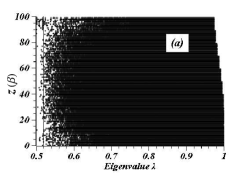
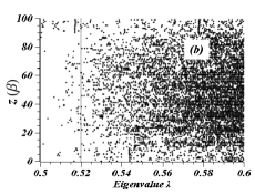
Figure 5: The three-parameter receiver state-space $(\lambda,\beta_{1},\beta_{2})$ (the black points) of map (40-40) for the four node chain with the two-qubit sender and the pure initial state ($\lambda^{B}=1$) is considered at $t_{0}=6.4$. Here we combine the parameters $\beta_{1}$ and $\beta_{2}$ in the single parameter $z(\beta)=10[10\beta_{1}]+[10\beta_{2}]$. Apparently, the region of the available states is uniform in $\beta_{2}$, which is confirmed by the step-like behavior of the right boundary of the creatable region. (a) The whole creatable region of the receiver’s state-space. (b) The hardly available area of the creatable states (the vertical stripe to the left from the dashed line). (c) The right boundary of the creatable region.

We see in Fig.5 that there is a region in the state-space which may not be created by the local transformations of the subsystem $A$ (the right upper corner in Figs.5a,c). This is the unavailable region associated with the initial state (36) and $\lambda^{B}=1$. Other initial states might have different unavailable regions. There is another region in Fig.5 which is hardly creatable. Conditionally, this region may be taken as a vertical stripe $\frac{1}{2}\leq\lambda\leq 0.52$, see the left side from the dotted line in Figs.5a,b. We shell give a following remark. Although we select the parameters $\varphi_{10}$, $\varphi_{11}$ and $\varphi_{12}$ in map (40), the similar results (concerning the state transfer with $\lambda^{B}=1$) are obtained for the other selected triad of parameters: ($\varphi_{1}$, $\varphi_{2}$, $\varphi_{3}$), ($\varphi_{3}$, $\varphi_{4}$, $\varphi_{5}$), ($\varphi_{5}$, $\varphi_{6}$, $\varphi_{7}$), ($\varphi_{7}$, $\varphi_{8}$, $\varphi_{9}$), ($\varphi_{9}$, $\varphi_{10}$, $\varphi_{11}$). This fact supports our assumption that simplified map (40) produces the maximal possible creatable region for the given choice of initial conditions.

Now, considering map (42), we clarify our choice of the time instant $t_{0}=6.4$. It is reasonable to select such a time instant for the state registration that corresponds to the maximal region creatable by map (42). Generally speaking, this instant depends on the value of $\lambda^{B}$ in initial state (36). However, to simplify the analysis, we use the same time instant $t_{0}$ for all values $\lambda^{B}$. Namely, let $t_{0}$ correspond to the maximal creatable region obtained with $\lambda^{B}=1$ (a pure initial state). This value may be simply found from the numerical simulations of the creatable regions at different time instants inside of the interval $[0,T\approx 10.2]$. As a result, we obtain $t_{0}\approx 6.4$.

References

- (1)
- (2) C.H.Bennett, G.Brassard, C.Crépeau, R.Jozsa, A.Peres, and W.K.Wootters, Phys. Rev. Lett. 70, 1895 (1993)
- (3) D.Bouwmeester, J.-W. Pan, K.Mattle, M.Eibl, H.Weinfurter, and A. Zeilinger, Nature 390, 575 (1997)
- (4) D. Boschi, S. Branca, F.De Martini, 1L. Hardy, and S. Popescu, Phys. Rev. Lett. 80, 1121 (1998)
- (5)
- (6) B.Yurke, D.Stoler, Phys. Rev. A 46, 2229 (1992)
- (7) B.Yurke, D.Stoler, Phys. Rev. Lett. 68, 1251 (1992)
- (8) M.Zukowski, A.Zeilinger, M.A.Horne, A.Ekert, Phys. Rev. Lett. 71, 4287 (1993)
- (9)
- (10) C.H.Bennett, D.P.DiVincenzo, P.W.Shor, J.A.Smolin, B.M.Terhal, and W.K.Wootters, Phys.Rev.Lett. 87, 077902 (2001); Erratum Phys. Rev. Lett. bf 88, 099902 (2002)
- (11)
- (12) C.H.Bennett, P.Hayden, D.W.Leung, P.W.Shor, and A.Winter, IEEE Transetction on Information Theory 51, 56 (2005)
- (13) N.A.Peters, J.T.Barreiro, M.E.Goggin, T.-C.Wei, and P.G.Kwiat, Phys.Rev.Lett. 94, 150502 (2005)
- (14) N.A.Peters, J.T.Barreiro, M.E.Goggin, T.-C.Wei, and P.G.Kwiat in Quantum Communications and Quantum Imaging III, ed. R.E.Meyers, Ya.Shih, Proc. of SPIE 5893 (SPIE, Bellingham, WA, 2005)
- (15) B.Dakic, Ya.O.Lipp, X.Ma, M.Ringbauer, S.Kropatschek, S.Barz, T.Paterek, V.Vedral, A.Zeilinger, C.Brukner, and P.Walther, Nat. Phys. 8, 666 (2012).
- (16) G.-Yo.Xiang, J.Li, B.Yu, and G.-C.Guo Phys. Rev. A 72, 012315 (2005)
- (17) G.L.Giorgi, Phys. Rev. A 88, 022315 (2013)
- (18) S. Bose, Phys. Rev. Lett. 91, 207901 (2003)
- (19) M.Christandl, N.Datta, A.Ekert and A.J.Landahl, Phys.Rev.Lett. 92, 187902 (2004)
- (20) C.Albanese, M.Christandl, N.Datta and A.Ekert, Phys.Rev.Lett. 93, 230502 (2004)
- (21) P.Karbach and J.Stolze, Phys.Rev.A 72, 030301(R) (2005)
- (22) E.I.Kuznetsova and E.B.Fel’dman, J.Exp.Theor.Phys. 102, 882 (2006)
- (23) E.I.Kuznetsova and A.I.Zenchuk, Phys.Lett.A 372, pp.6134-6140 (2008)
- (24) G.Gualdi, V.Kostak, I.Marzoli and P.Tombesi, Phys.Rev. A 78, 022325 (2008)
- (25) E.B.Fel’dman and A.I.Zenchuk, Phys. Lett. A 373 (2009) 1719
- (26) A.Wójcik, T.Luczak, P.Kurzyński, A.Grudka, T.Gdala, and M.Bednarska Phys. Rev. A 72, 034303 (2005)
- (27) S.I.Doronin, A.I.Zenchuk, Phys. Rev. A 81, 022321 (2010)
- (28) G. De Chiara, D. Rossini, S. Montangero, R. Fazio, Phys. Rev. A 72, 012323 (2005)
- (29) A. Zwick, G.A. Álvarez, J. Stolze, O. Osenda, Phys. Rev. A 84, 022311 (2011)
- (30) A. Zwick, G.A. Álvarez, J. Stolze, O. Osenda, Phys. Rev. A 85, 012318 (2012)
- (31) A. Zwick, G.A. Álvarez, J. Stolze, O Osenda, arXiv preprint arXiv:1306.1695, (2013)
- (32) J.Stolze, G. A. Álvarez, O. Osenda, A. Zwick in Quantum State Transfer and Network Engineering. Quantum Science and Technology, ed. by G.M.Nikolopoulos and I.Jex, Springer Berlin Heidelberg, Berlin, p.149 (2014)
- (33) E.B.Fel’dman,E.I.Kuznetsova and A.I.Zenchuk, Phys.Rev.A 82 (2010) 022332
- (34) A.I.Zenchuk, J. Phys. A: Math. Theor. 45 (2012) 115306
- (35) L.Campos Venuti, S.M.Giampaolo, F.Illuminati, P.Zanardi, Phys. Rev. A 76, 052328 (2007)
- (36) G.Gualdi, I.Marzoli, P.Tombesi, New J. Phys. 11, 063038 (2009)
- (37) A.Bayat and S.Bose, Phys. Rev. A 81, 012304 (2010)
- (38) S.I.Doronin, E.B.Fel’dman, and A.I.Zenchuk, Phys. Rev. A 79, 042310 (2009)
- (39) A.I.Zenchuk, ”Informational correlation between two parties of a quantum system. Spin-1/2 chains”, to appear in Quant. Inf. Proc., arXiv:1307.0272 [quant-ph]
- (40) W.K. Wootters,, Phys. Rev. Lett. 80, 2245 (1998)
- (41) S.Hill and W.K.Wootters, Phys. Rev. Lett. 78, 5022 (1997)
- (42) A.Peres, Phys. Rev. Lett. 77, 1413 (1996)
- (43) L.Amico, R.Fazio, A.Osterloh and V.Ventral, Rev. Mod. Phys. 80, 517 (2008)
- (44) R.Horodecki, P.Horodecki, M.Horodecki and K.Horodecki, Rev. Mod. Phys. 81, 865 (2009)
- (45) L. Henderson, V. Vedral, J. Phys. A: Math. Gen. 34, 6899 (2001)
- (46) H.Ollivier and W.H.Zurek, Phys.Rev.Lett. 88, 017901(2001)
- (47) W.H. Zurek, Rev. Mod. Phys. 75, 715 (2003)
- (48) T.Tilma, M.Byrd and E.C.G.Sudarshan, J.Phys.A:Math.Gen. 35, 10445 (2002)
- (49) A.I.Zenchuk, arXiv:1307.0272 [quant-ph]
- (50) W.Greiner and B.Müller: Quantum Mechanics: Symmetries, (Springer, Berlin 1989)