The Mean Interference-to-Signal Ratio and its
Key Role in Cellular and Amorphous Networks

Abstract

We introduce a simple yet powerful and versatile analytical framework to approximate the SIR distribution in the downlink of cellular systems. It is based on the mean interference-to-signal ratio and yields the horizontal gap (SIR gain) between the SIR distribution in question and a reference SIR distribution. As applications, we determine the SIR gain for base station silencing, cooperation, and lattice deployment over a baseline architecture that is based on a Poisson deployment of base stations and strongest-base station association. The applications demonstrate that the proposed approach unifies several recent results and provides a convenient framework for the analysis and comparison of future network architectures and transmission schemes, including amorphous networks where a user is served by multiple base stations and, consequently, (hard) cell association becomes obsolete.

I Introduction

I-A Motivation and contribution

The SIR distribution is a key metric in interference-limited wireless systems. Due to high capacity demands and limited spectrum, current- and next-generation cellular systems adopt aggressive frequency reuse schemes, which makes interference the main performance-limiting factor. To overcome coverage and capacity problems due to interference, many sophisticated transmission schemes, including base station cooperation and silencing, successive interference cancellation, multi-user MIMO, and multi-tier architectures have recently been proposed. However, a simple evaluation and comparison of their effect on the SIR distribution has been elusive.

In this paper, we propose a novel technique that provides tight approximations of the SIR gain of advanced downlink architectures and cooperation schemes over a baseline scheme. It is based on the mean interference-to-signal ratio (MISR), which is used to quantify the horizontal gap between two SIR distributions. To account for the spatial irregularity of current and future cellular system, we use point process models for the positions of the base stations (BSs) [1, 2].

I-B The horizontal gap in the SIR distribution

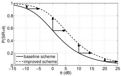
We focus on the complementary cumulative distribution (ccdf) $\bar{F}_{\mathrm{SIR}}(\theta)\triangleq\mathbb{P}(\mathrm{SIR}>\theta)$ of the SIR. There are two ways to compare SIR distributions, vertically or horizontally, see Fig. 1 for an illustration. Using the vertical gap, i.e., the gain in the coverage probability, has several disadvantages: (1) it depends strongly on the value of $\theta$ where it is evaluated; (2) it is often unclear whether the gain is measured in absolute or relative terms (for example, at -10 dB, the gap is 0.058, or 6.4%; at 0 dB, the gap is 0.22, or 39%, and at 20 dB, the gap is 0.05, or 78%—and sometimes even the absolute gain is expressed in percentages); (3) the gain also depends heavily on the path loss law and fading models.

In contrast, the horizontal gap (SIR gain) is often quite insensitive to the probability where it is evaluated and the path loss models. Formally, the gap between the distributions of $\mathrm{SIR}_{1}$ and $\mathrm{SIR}_{2}$ is defined as

$$G(p)\triangleq\frac{\bar{F}_{\mathrm{SIR}_{2}}^{-1}(p)}{\bar{F}_{\mathrm{SIR}_{1}}^{-1}(p)},\quad p\in(0,1),$$ (1)

where $\bar{F}_{\mathrm{SIR}}^{-1}$ is the inverse of the ccdf of the $\mathrm{SIR}$, and $p$ is the target success probability. In Fig. 1, for example, $G(p)=5$dB, irrespective of $p$. In the following, we will illustrate that this behavior is commonly observed. We also define the asymptotic gain (whenever the limit exists) as

$$G\triangleq G(1)=\lim_{p\to 1}G(p).$$ (2)

Figure 1: Example SIR ccdfs for a baseline and an improved scheme. The vertical gap between the distributions depends strongly on the value of $\theta$ where it is evaluated, while the horizontal gap is almost constant.

II The Mean Interference-to-Signal Ratio and its Significance

II-A Definition

We first define the interference-to-average-signal ratio $\mathrm{I{\bar{S}}R}$.

Definition 1 ($\mathrm{I{\bar{S}}R}$)

The interference-to-average-signal ratio $\mathrm{I{\bar{S}}R}$ is defined as

$$\mathrm{I{\bar{S}}R}\triangleq\frac{I}{\mathbb{E}_{h}(S)},$$

where $I$ is the sum power of all interferers and $\bar{S}=\mathbb{E}_{h}(S)$ is the signal power averaged over the fading. Its mean is denoted by $\mathrm{MISR}\triangleq\mathbb{E}(\mathrm{I{\bar{S}}R})$.

The bar over the $S$ in the $\mathrm{I{\bar{S}}R}$ indicates averaging over the fading. The $\mathrm{I{\bar{S}}R}$ is a random variable due to the random positions of the BSs relative to the typical user. For the following discussion, we assume a power path loss law $\ell(r)=r^{-\alpha}$ with a path loss exponent $\alpha$ and (power) fading with unit mean, i.e., for all fading random variables, $\mathbb{E}(h)=1$. We also assume that the desired signal comes from a single BS at distance $R$, while the interferers are located at distances $R_{k}$ and their transmit powers (relative to the one of the serving BS) are $P_{k}$. In this case, the $\mathrm{I{\bar{S}}R}$ is given by

$$\mathrm{I{\bar{S}}R}=R^{\alpha}\sum_{k\in\mathcal{I}}h_{k}P_{k}R_{k}^{-\alpha},$$

where $\mathcal{I}$ is the index set of the interferers and $h_{k}$ denotes the channel (power) gain. The mean follows as

$$\mathrm{MISR}\triangleq\mathbb{E}(\mathrm{I{\bar{S}}R})=\sum_{k\in\mathcal{I}}P_{k}\mathbb{E}\left(\frac{R^{\alpha}}{R_{k}^{\alpha}}\right).$$

So the $\mathrm{MISR}$ is a function of the distance ratios $R_{k}/R$ between the desired and interfering base stations, scaled by the relative transmit powers.

II-B The asymptotic gap for Rayleigh fading

The SIR distribution can be expressed using the $\mathrm{I{\bar{S}}R}$ as

$$F_{\mathrm{SIR}}(\theta)=\mathbb{P}(h\bar{S}<\theta I)=\mathbb{P}(h<\theta\,\mathrm{I{\bar{S}}R}).$$

For exponential $h$ and $\theta\to 0$,

$$\mathbb{P}(h<\theta\,\mathrm{I{\bar{S}}R}\mid\mathrm{I{\bar{S}}R})\sim\theta\,\mathrm{I{\bar{S}}R},$$

thus

$$\mathbb{P}(h<\theta\,\mathrm{I{\bar{S}}R})\sim\theta\,\mathbb{E}(\mathrm{I{\bar{S}}R}).$$

So $F_{\mathrm{SIR}}(\theta)\sim\theta\,\mathrm{MISR}$, and $\bar{F}_{\mathrm{SIR}}^{-1}(p)\sim(1-p)/\mathrm{MISR}$, $p\to 1$. Consequently, the asymptotic gain between two SIR ccdfs (2) can be expressed as

$$G=\frac{\mathrm{MISR}_{1}}{\mathrm{MISR}_{2}},$$ (3)

and if it is finite, we have $\bar{F}_{\mathrm{SIR}_{1}}(\theta)\sim\bar{F}_{\mathrm{SIR}_{2}}(\theta/G)$, $\theta\to 0$.

We will demonstrate in the next section that this relationship provides an accurate approximation for the gain also at non-vanishing values of $\theta$, i.e., that $\bar{F}_{\mathrm{SIR}}(\theta)\approx\bar{F}_{\mathrm{SIR}}(\theta/G)$ for all practical values of $\theta$.

Other types of fading will be discussed in Sec. IV.

II-C The HIP model and the baseline MISR

The homogeneous independent Poisson (HIP) model was first introduced as a model for cellular networks in [1].

Definition 2 (HIP Model)

A homogeneous independent Poisson (HIP) model with $n$ tiers consists of $n$ independent Poisson point processes (PPPs) $\Phi_{k}\subset\mathbb{R}^{2}$ with intensities $\lambda_{k}$, $k\in[n]$ and power levels $P_{k}$. $\Phi_{k}$ is the set of locations of the base stations of the $k$-th tier.

Remarks:

• Alternatively, the HIP model can be defined as follows: Let $\lambda=\sum_{k\in[n]}\lambda_{k}$. Starting with a homogeneous Poisson point process (PPP) $\Phi\subset\mathbb{R}^{2}$ of intensity $\lambda$, randomly assign each point $x\in\Phi$ to one of the $k$ tiers $\Phi_{k}$, where $\mathbb{P}(x\in\Phi_{k})=\lambda_{k}/\lambda$, independently for each $x$.

• Although the HIP model is a model for a heterogeneous network, we call it homogeneous, since it is based on homogeneous PPPs, i.e., the base stations form a spatially homogeneous point process.

• The HIP model is doubly independent, since it exhibits neither intra-tier nor inter-tier dependence. This makes it highly tractable but also makes it less accurate in situations where base stations are deployed in a repulsive fashion (i.e., with a certain minimum distance) [3] or where base stations of different tiers are not placed independently [4].

• Quite remarkably, for the power path loss law with Rayleigh fading and with strongest-BS association (on average, i.e., not considering small-scale fading), the SIR distribution for the HIP model does not depend on the number of tiers $n$, their densities $\lambda_{k}$, or their power levels $P_{k}$ [5]. For $\alpha=4$, the SIR distribution is given by the extremely simple expression

  $$\bar{F}_{\mathrm{SIR}[4]}(\theta)=\frac{1}{1+\sqrt{\theta}\arctan\sqrt{\theta}}.$$ (4)

  Also, $\mathbb{E}(S)=\infty$ and $\mathbb{E}(\mathrm{SIR})=\infty$ for all values of $\alpha$ due to the proximity of the nearest BS, and $\mathbb{E}(I)=\infty$ for $\alpha\geq 4$.

Due to its tractability, the HIP model with strongest-base station association is the perfect candidate for a baseline model against which the gains of other schemes can be measured. Since the SIR distribution does not depend on the density or number of tiers, we use a single-tier model in the following to calculate the MISR for the HIP model.

Let $R_{k}$ be the distance from the typical user to the $k$-th nearest BS. Its distribution is given by [6]. The distribution of the distance ratio $\nu_{k}=R_{1}/R_{k}$ is [7, Lemma 3]

$$F_{\nu_{k}}(x)=1-(1-x^{2})^{k-1},\quad x\in[0,1],$$

and the $\alpha$-th moments are

$$\mathbb{E}(\nu_{k}^{\alpha})=\frac{\Gamma(1+\alpha/2)\Gamma(k)}{\Gamma(k+\alpha/2)}.$$ (5)

For equal powers $P_{k}\equiv 1$, the MISR follows as

$$\mathbb{E}(\mathrm{I{\bar{S}}R})=\sum_{k=2}^{\infty}\frac{\Gamma(1+\alpha/2)\Gamma(k)}{\Gamma(k+\alpha/2)}=\frac{2}{\alpha-2},\quad\alpha>2.$$ (6)

For $\alpha=4$, $\mathrm{MISR}=1$, which implies $F_{\mathrm{SIR}}(\theta)\sim\theta$, $\theta\to 0$.

III Applications

III-A Base station silencing

We consider the (single-tier) HIP model and let $\mathrm{I{\bar{S}}R}^{(!n)}$ denote the $\mathrm{I{\bar{S}}R}$ if the $n$ strongest interfering BSs (on average) are silenced, and all BSs transmit at the same power.

If the nearest interfering BS is silenced, the MISR is obtained by subtracting $\mathbb{E}(\nu_{2}^{\alpha})$ from (6), which yields

$$\mathbb{E}(\mathrm{I{\bar{S}}R}^{(!1)})=\frac{2}{\alpha-2}-\frac{2}{\alpha+2}=\frac{8}{\alpha^{2}-4}.$$

For general $n$,

$$\mathbb{E}(\mathrm{I{\bar{S}}R}^{(!n)})=\frac{2\Gamma(1+\alpha/2)}{\alpha-2}\,\frac{\Gamma(n+2)}{\Gamma(n+1+\alpha/2)}.$$

The same result has been obtained in [7, Prop. 1] by calculating the limiting outage probability $F_{\mathrm{SIR}}(\theta)$ as $\theta\to 0$.

For $\alpha=4$, $\mathbb{E}(\mathrm{I{\bar{S}}R}^{(!n)})=\frac{2}{n+2}$, and the asymptotic gain per (3) is simply

$$G_{\rm silence[4]}=\frac{1}{\mathbb{E}(\mathrm{I{\bar{S}}R}^{(!n)})}=1+\frac{n}{2}.$$

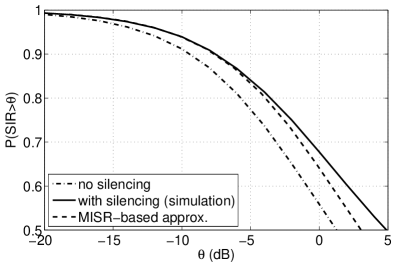
Fig. 2 shows the SIR distributions for the HIP model without silencing, for the HIP model with silencing of one BS, and the MISR-based approximation. The approximation is tight for success probabilities above $3/4$; after that, it is pessimistic.

Figure 2: Gain from silencing one base station in HIP model for $\alpha=4$.

III-B Base station cooperation for worst-case users

We focus on worst-case users in the single-tier HIP model, which are the ones located at the vertices of the Voronoi tessellation [9, 5]. These locations are marked by $\times$ in Fig. 3, and the SIR ccdf is denoted as $\bar{F}_{\mathrm{SIR}}^{\times}$ accordingly. Worst-case users are at a significant disadvantage if they are served by a single BS since they have two other BSs at the same distance.

With (non-coherent) joint transmission from the 3 equidistant BSs and $\alpha=4$, the ccdf follows from [5, Thm. 2] as

$$\bar{F}_{\mathrm{SIR}[4]}^{{\times,{\rm coop}}}(\theta)=\bar{F}_{\mathrm{SIR}[4]}^{{2}}(\theta/{3})=\Big{(}1+\sqrt{\theta/{3}}\arctan(\sqrt{\theta/{3}})\Big{)}^{-2}.$$ (7)

where $\bar{F}_{\mathrm{SIR}[4]}$ is the SIR ccdf for the typical user in the HIP model given in (4). The factor of $3$ is due to the gain in signal power, while the exponent of 2 is due to the larger distance of the nearest BS than in the case of the typical user.

Without cooperation, $\mathrm{MISR}^{\times}=2+4/(\alpha-2)$, and for $n\in\{2,3\}$ BSs cooperating, it follows from [5, Thm. 4] that

$$\mathrm{MISR}^{\times}_{n-{\rm coop}}=\frac{4+(3-n)(\alpha-2)}{n(\alpha-2)}.$$

So for $n=3$, the gain is

$$G_{3-{\rm coop}}=\frac{{\rm MISR}^{\times}}{\rm MISR_{3-coop}^{\times}}=3+\frac{3}{2}(\alpha-2).$$

Fig. 4 shows the SIR distribution for worst-case users without cooperation, with cooperation from the 3 nearest BSs, and the MISR-based approximation.

Figure 3: Illustration of worst-case user locations. Base stations are marked by $\odot$, and the crosses $\times$ are the vertices of the Voronoi tessellation and mark the locations of the worst-case users. These users have the same distance to the 3 nearest BSs.

Figure 4: SIR ccdf for worst-case users without cooperation and with 3-BS cooperation (from (7)) and MISR-based approximation for $\alpha=4$. Here $G=6$ (7.8 dB).

III-C Non-Poisson deployment

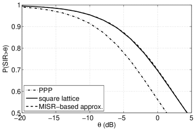
An SIR gain can also be obtained by deploying the BSs more regularly (repulsively) than a PPP. This gain has been termed deployment gain in [10, 8]. Exact closed-form results for the SIR distribution for non-Poisson deployments are impossible to derive. However, the MISR-based approximation, relative to the HIP model, is fairly easy to evaluate and quite accurate.

Simulations show that the MISR of the square lattice is quite exactly half of that of the PPP, irrespective of the path loss exponent, i.e., the deployment gain is 3 dB. Fig. 5 shows that the resulting approximation is accurate over a wide range of $\theta$. As a result,

$$\bar{F}_{\mathrm{SIR}[4]}^{\rm sq}(\theta)\approx\bar{F}_{\mathrm{SIR}[4]}(\theta/2),$$

where $\bar{F}_{\mathrm{SIR}[4]}$ is given in (4), is a very good analytical approximation to the SIR distribution in the square lattice. For the triangular lattice (hexagonal cells), the gain is slightly larger, about 3.4 dB, which is the maximum achievable.

Figure 5: SIR ccdf for the square lattice and MISR-based approximation for $\alpha=4$ (Rayleigh fading).

IV General fading and diversity

So far we have discussed the case of Rayleigh fading. The MISR framework easily extends to other types of fading or transmission schemes with diversity (e.g., coherent BS cooperation, MIMO, retransmission). The diversity under interference (DUI) is defined as [11, 7]

$$d\triangleq\lim_{\theta\to 0}\frac{\log F_{\mathrm{SIR}}(\theta)}{\log\theta}.$$

When comparing SIR distributions, the two schemes need to provide the same diversity gain $d$ (i.e., have the same asymptotic slope in the outage curve when plotted on a log-log scale), otherwise the asymptotic gain may be undefined or not helpful in approximating one ccdf with the other.

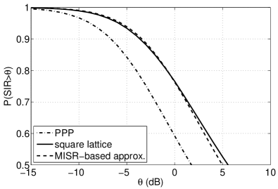
For example, if the fading distribution satisfies $F_{h}(x)\sim ax^{m}$, $x\to 0$, (as, e.g., in Nakagami-$m$ fading)

$$F_{\mathrm{SIR}}(\theta)\sim a\theta^{m}\mathbb{E}(\mathrm{I{\bar{S}}R}^{m}),$$

the diversity order is $m$—if the $m$-th moment of the $\mathrm{I{\bar{S}}R}$ is finite. The asymptotic gain follows as

$$G^{(m)}=\left(\frac{\mathbb{E}(\mathrm{I{\bar{S}}R}_{1}^{m})}{\mathbb{E}(\mathrm{I{\bar{S}}R}_{2}^{m})}\right)^{1/m}\approx G^{(1)},$$

where the approximation by $G^{(1)}$ holds since the factor $\mathbb{E}(\mathrm{I{\bar{S}}R}^{m})^{1/m}/\mathrm{MISR}$ is about the same for both schemes and thus cancels approximately. This is illustrated in Fig. 6 for Nakagami-2 fading and the square lattice. The shift by $G^{(1)}=3$ dB still yields a very good approximation.

Figure 6: SIR ccdf of square lattice and MISR-based approximation for $\alpha=4$ and Nakagami-2 fading.

V Conclusions

The SIR distributions of two transmission schemes or deployments in cellular networks that provide the same diversity gain are, asymptotically, horizontally shifted version of each other, and the asymptotic gap between them is quantified by the ratio of the MISRs of the two schemes. We demonstrated that this asymptotic gap also provides a good approximation for the gap at finite $\theta$.

If the MISR cannot be calculated analytically, it is relatively easy to determine by simulation since it only depends on the BS and user locations and the transmit power levels, but not on the fading. Due to its tractability, the HIP model is the prime candidate as a baseline model against which other schemes can be evaluated. So even if it is not be accurate in all situations, it serves the important role of a reference model.

We anticipate that future networks will not be based on a strict cellular architecture but will become amorphous due to cooperation between BSs at different levels, relays, and distributed antenna systems. Since an exact analytical evaluation for the SIR distribution for these sophisticated and cognitive architectures seems hopeless, we believe that the proposed MISR framework will play an important role in the analysis of such emerging amorphous networks.

References

- [1] H. S. Dhillon, R. K. Ganti, F. Baccelli, and J. G. Andrews, “Modeling and Analysis of K-Tier Downlink Heterogeneous Cellular Networks,” IEEE Journal on Selected Areas in Communications, vol. 30, pp. 550–560, Mar. 2012.
- [2] H. ElSawy, E. Hossain, and M. Haenggi, “Stochastic Geometry for Modeling, Analysis, and Design of Multi-tier and Cognitive Cellular Wireless Networks: A Survey,” IEEE Communications Surveys & Tutorials, vol. 15, pp. 996–1019, July 2013.
- [3] N. Deng, W. Zhou, and M. Haenggi, “The Ginibre Point Process as a Model for Wireless Networks with Repulsion,” IEEE Transactions on Wireless Communications, 2014. Submitted. Available at http://www.nd.edu/~mhaenggi/pubs/twc14c.pdf.
- [4] N. Deng, W. Zhou, and M. Haenggi, “A Heterogeneous Cellular Network Model with Inter-tier Dependence,” in IEEE Global Communications Conference (GLOBECOM’14), (Austin, TX), Dec. 2014. Submitted. Available at http://www.nd.edu/~mhaenggi/pubs/globecom14a.pdf.
- [5] G. Nigam, P. Minero, and M. Haenggi, “Coordinated Multipoint Joint Transmission in Heterogeneous Networks,” IEEE Transactions on Communications, 2014. Submitted. Available at http://www.nd.edu/~mhaenggi/pubs/tcom14.pdf.
- [6] M. Haenggi, “On Distances in Uniformly Random Networks,” IEEE Transactions on Information Theory, vol. 51, pp. 3584–3586, Oct. 2005.
- [7] X. Zhang and M. Haenggi, “A Stochastic Geometry Analysis of Inter-cell Interference Coordination and Intra-cell Diversity,” IEEE Transactions on Wireless Communications, 2013. Submitted. Available at http://www.nd.edu/~mhaenggi/pubs/twc14b.pdf.
- [8] A. Guo and M. Haenggi, “Asymptotic Deployment Gain: A Simple Approach to Characterize the SINR Distribution in General Cellular Networks,” IEEE Transactions on Communications, 2014. Submitted. Available at http://www.nd.edu/~mhaenggi/pubs/tcom14b.pdf.
- [9] S. Y. Jung, H.-K. Lee, and S.-L. Kim, “Worst-Case User Analysis in Poisson Voronoi Cells,” IEEE Communications Letters, vol. 17, pp. 1580–1583, Aug. 2013.
- [10] A. Guo and M. Haenggi, “Spatial Stochastic Models and Metrics for the Structure of Base Stations in Cellular Networks,” IEEE Transactions on Wireless Communications, vol. 12, pp. 5800–5812, Nov. 2013.
- [11] M. Haenggi and R. Smarandache, “Diversity Polynomials for the Analysis of Temporal Correlations in Wireless Networks,” IEEE Transactions on Wireless Communications, vol. 12, pp. 5940–5951, Nov. 2013.