A Critical Review of Classical Bouncing Cosmologies
Abstract
Given the proliferation of bouncing models in recent years, we gather and critically assess these proposals in a comprehensive review. The PLANCK data shows an unmistakably red, quasi scale-invariant, purely adiabatic primordial power spectrum and no primary non-Gaussianities. While these observations are consistent with inflationary predictions, bouncing cosmologies aspire to provide an alternative framework to explain them. Such models face many problems, both of the purely theoretical kind, such as the necessity of violating the NEC and instabilities, and at the cosmological application level, as exemplified by the possible presence of shear. We provide a pedagogical introduction to these problems and also assess the fitness of different proposals with respect to the data. For example, many models predict a slightly blue spectrum and must be fine-tuned to generate a red spectral index; as a side effect, large non-Gaussianities often result.
We highlight several promising attempts to violate the NEC without introducing dangerous instabilities at the classical and/or quantum level. If primordial gravitational waves are observed, certain bouncing cosmologies, such as the cyclic scenario, are in trouble, while others remain valid. We conclude that, while most bouncing cosmologies are far from providing an alternative to the inflationary paradigm, a handful of interesting proposals have surfaced, which warrant further research. The constraints and lessons learned as laid out in this review might guide future research.
pacs:
98.80.Es, 98.80.Cq, 98.80.-kI Introduction
It is often stated nowadays that cosmology has entered a regime of precision somewhat comparable to particle physics Mukhanov (2005); Peter and Uzan (2009). Although probably an exaggeration, there is a grain of truth in such a statement: based on the PLANCK data111We also take into consideration the BICEP2 data Ade et al. (2014a), pending independent confirmation., researchers have begun not only to discriminate between frameworks, but also to argue in favor of specific mechanisms. Indeed, with a purely Gaussian signal and a scalar spectral index strictly less than unity (at the level), but close to scale invariance, and no isocurvature contribution at any detectable level, it is hard to imagine any mechanism not based on quantum vacuum fluctuations of a single effective scalar field. Inflation Guth (1981) thus appears, contrary to what has been stated Ijjas et al. (2013, 2014a), the most fashionable Linde (2008); Lemoine et al. (2008); Baumann (2009); Martin et al. (2014a, b); Baumann and McAllister (2014) and some might say natural Guth et al. (2014); Linde (2014) candidate to explain the data (it has been argued that inflation with its wide range of possible predictions is unverifiable and thus untenable and not in the realm of science; if such an argument were valid, the same could be said about the quantum field theory paradigm, which also needs a specific implementation to be put to the test experimentally – see also Barrow and Liddle (1997)).
Being the most fashionable candidate, however, does not make inflation true, and before we can confidently say that a phase of inflation took place, assuming there will ever be such a time, we need to make sure that all other possibilities are ruled out. To our knowledge, this is the case for most of the other proposals to generate large scale structures, such as seeding fluctuations by a cosmic string network Ringeval et al. (2007); Peter and Ringeval (2013); Ade et al. (2013a). Apart from models of an emerging universe in string gas cosmology Battefeld and Watson (2006); Brandenberger et al. (2014), all viable nonsingular alternatives to date replace the primordial singularity by a bounce connecting a contracting phase to the currently expanding one.
We concentrate on pure alternatives to inflation, i.e. we do not consider the otherwise well-justified models in which a bounce is followed by a phase of inflation Piao et al. (2004); Falciano et al. (2008); Lilley et al. (2011); Liu et al. (2013); Biswas and Mazumdar (2014). Such models naturally get the best of both ideas and should be considered in view of addressing the question of the primordial singularity in the inflationary paradigm.
The purpose of this work is to review models that aim to explain observations by mechanisms in a bouncing universe and to provide a critical assessment. We believe it is useful to know not only the strength but also the weaknesses of a given approach to find possible cures and to yield a better understanding of these models. If all possible alternatives turn out to be irreconcilable with the given data, the inflationary paradigm would not be proven, but our confidence in it would increase considerably; if the primordial gravitational wave background level is sufficiently high, as would be the case if Ade et al. (2014a) and its interpretation is confirmed, there is hope to verify the inflationary consistency relation between the tensor spectral index and the tensor-to-scalar ratio ; this would put all models featured in this review in difficulty.
I.1 Why is there a necessity for alternative models to inflation?
How can we accurately describe the 13.8 billion year evolution of our Universe? The standard model of the early Universe can be traced back to several seminal observations: galaxies are receding faster the further away they are, indicating an expanding universe Hubble (1929); the cosmic microwave background radiation (CMBR) is highly isotropic and the expansion is accelerating Perlmutter et al. (1999); Riess et al. (1998); this acceleration is attributed to an unknown component, dark energy. Big bang cosmology accounts for the Hubble expansion and predicts the existence of the CMBR. The abundance of light elements can be computed, and their values agree with observations, with the possible exception of 7Li (see Coc et al. (2014) for a recent review). Moreover, numerical simulations Teyssier et al. (2009) of large scale structure formation based on what we believe to be the relevant initial conditions, as deduced from the properties of the CMBR, reproduce well the observed features of the actual distribution: at first sight, the standard hot big bang model successfully provides a description of the Universe back to a fraction of a second after its birth until today with amazing precision; it is hard to overestimate the success that such a model represents in a science that a century ago did not exist.
However successful from a fraction of a second onward, the simple hot big bang model is plagued by several problems when extrapolated backwards in time: it begins with an initial singularity leading to a tiny horizon, without an explanation for the vanishingly small spatial curvature, it does not explain why baryons should have been formed in an asymmetric way (with respect to antibaryons), why exotic relics are absent or how the density fluctuations, from which large-scale structures developed, are seeded. Most of these problems can be addressed by postulating an inflationary phase Guth (1981), i.e. a period of accelerated expansion taking place during the early stages of our Universe; however, the existence of a primeval singularity is not modified in the inflationary framework, which remains geodesically incomplete Borde and Vilenkin (1996).
Originally conceived in order to rid the hot big bang model from the Grand Unified Theory (GUT) monopole problem, inflation has rapidly been developed to become a paradigm of modern theoretical cosmology. The simplest models of inflation not only solve the horizon and flatness problems, but they also predict, as an initially unexpected bonus, the statistical properties of temperature fluctuations in the CMBR, in full agreement with the most recent observations. However, from a theoretical point of view, inflation is not free of problems. First, in large field models of inflation, the inflaton has to traverse a distance in field space larger than the Planck mass in natural units. This has been argued to be problematic, since non-renormalizable quantum corrections to the field’s action arise. In the absence of functional fine-tuning or additional symmetries, inflation would be spoiled; this is known as the problem of inflation. Small field models are more appealing, but also fine-tuned, for instance to account for the proper amplitude of the power spectrum. An exhaustive review and comparison of single field models with the PLANCK data is given in Martin et al. (2014a, b). However, if the BICEP2 detection of gravitational waves were confirmed, all of these small field models would be in trouble Martin et al. (2014c). Foreground emission studies using the BICEP1 and BICEP2 data suggest that the background and a gravitational wave signal are indistinguishable in this region Flauger et al. (2014); Mortonson and Seljak (2014). See Sec.IV.4 for more details and Baumann and McAllister (2014) for a recent review of inflation in string theory post BICEP2. Second, the presence of eternal inflation in almost all proposals has been argued to lead to a possible loss of predictability due to our inability to prescribe a unique measure Ijjas et al. (2013, 2014a): this is the so-called measure problem (see however Guth et al. (2014); Linde (2014)). Third, inflation does not provide a theory of initial conditions that would explain why the inflaton field starts out high in its potential. A related issue is the low initial entropy of the initial state that has to be assumed, just as in big bang cosmology; this is known as the entropy problem. Fourth, the initial singularity, as visible in curvature invariants, does not disappear, but is merely pushed into the past; this may stem from the strict use of General Relativity (GR). Some of these problems could have an environmental solution in terms of the anthropic principle in a wide landscape of otherwise uninhabitable solutions. See Linde (2014) for a recent review on these topics; it should be noted that the measure problem may render a quantification of anthropic arguments challenging.
These problems of inflation have fueled the search for alternatives, most of which have not passed the CMBR constraints. A seemingly viable alternative, which also provides a GR-compatible solution to the singularity problem, relies on a nonsingular bouncing cosmology Brandenberger et al. (1993); Novello and Bergliaffa (2008), whereby an initially contracting phase connects with the currently expanding one through some minimal scale factor (and hence a vanishing Hubble rate). These models have a history that predates inflationary solutions by many decades, as they were proposed shortly after the first observations of the expansion Lemaitre (1927); Hubble (1929) by Tolman Tolman (1931) and Lemaître Lemaître (1933); Lemaitre (1997) (see also Barrow and Dabrowski (1995) for a more modern viewpoint concerning Tolman’s cyclic approach): at this time, the expansion appeared to imply that Einstein’s theory of gravity was doomed to fail, as the scale factor reaches infinitesimally small values, such that the Universe emerges from a primordial singularity. This singularity problem was ignored for many years as interest in cosmology faded among physicists, until it reemerged in the early 1980s Starobinskii (1978); Starobinsky (1980), when GR was again perceived as not only a mathematically entertaining theory, but also as a physically relevant description on large scales. Shortly thereafter, cosmological inflation was proposed Guth (1981), see Bassett et al. (2006); Lemoine et al. (2008); Baumann and McAllister (2014) for reviews, and bouncing cosmologies faded again into oblivion as researchers focused on developing the inflationary framework.
In parallel, string theorists investigated cosmological solutions in dilaton gravity, leading to the pre-big bang (PBB) scenario, which was the first attempt to implement a non singular bounce within this framework; Ref. Gasperini and Veneziano (2003) presents a comprehensive review of this model. The universe starts out empty and flat, with the dilaton in the weak coupling regime. As the dilaton evolves towards strong coupling, a transition from pre- to post big bang was though to occur in the strong coupling regime, which appears as a bounce in the Jordan frame (but not in the Einstein frame). While ultimately not a successful model of the early universe, as detailed in Ref. Gasperini and Veneziano (2003), the pre-big bang scenario paved the way for bouncing scenarios, which employ many of the ideas and techniques of the PBB. Thus, bouncing cosmologies resurfaced to provide a challenge or merely a working alternative to the inflationary paradigm, see e.g. Durrer and Laukenmann (1996); Peter and Pinto-Neto (2002a); Khoury et al. (2001a) among many other proposals. Over the last years, considerable effort has been made in developing well-behaved, nonsingular and singular bouncing models. Our goal is to critically review these new developments. A prior review Novello and Bergliaffa (2008) concentrated on quite different categories of models, while this work aims at discussing more widely held views.
I.2 What is used to get a bounce?
To achieve a bounce, the Hubble rate , which emerges from the contracting phase with a negative value, must increase, since it is positive during the subsequent expanding phase. There are two options to increase the Hubble rate from negative to positive: the first one operates within General Relativity and hence usually requires the violation of the null energy condition, NEC, Peter and Pinto-Neto (2002a): Einstein equations (6), as provided in the next section, indeed imply that the time derivative of the Hubble rate reads
| (1) |
so that when the spatial sections are flat (), definitely demands . A generic consequence of violating the null energy condition is the appearance of fields with negative kinetic energy: ghosts; a crucial point in bouncing models is actually to construct a regular model in which such ghosts are absent while still having a bouncing phase. It is possible to generate a bounce in the presence of curvature without violating the NEC, but only the strong energy condition, SEC, which demands and , see Martin and Peter (2003); Falciano et al. (2008) for concrete models. Such a bounce could leave some amount of spatial curvature in the expanding phase, whose amplitude may require a subsequent inflationary phase to dilute it, hence possibly ruining the alternative-to-inflation program (as emphasized above, we shall not be concerned here with the mixed models in which a bounce permits to avoid a primordial singularity while a subsequent inflation phase solves the other puzzles of the standard hot big-bang model).
The second option is to allow for a classically singular bounce. Here the scale factor actually vanishes and as such, four-dimensional General Relativity ceases to be valid close to the bounce. Pragmatically, the contracting phase is often matched to the expanding one within GR under the assumption that the actual bounce leaves observables unaffected. In the words of Xue and Steinhardt (2010): “[…] the Universe contracts towards a “big crunch” until the scale factor is so small that quantum gravity effects become important. The presumption is that these quantum gravity effects introduce deviations from conventional general relativity and produce a bounce that preserves the smooth, flat conditions achieved during the ultra-slow contraction phase”. One thus assumes all goes roughly unchanged on the cosmologically interesting scales through the otherwise quantum gravity dominated phase.
This matching procedure is not as easy as it appears at first sight, because ambiguities arise when trying to impose the Deruelle-Mukanov matching conditions to cosmological perturbations Deruelle and Mukhanov (1995); see Sec. IV.6. Attempts have been made to employ methods akin to the AdS/CFT correspondence to a singular bounce Craps et al. (2012, 2009); Smolkin and Turok (2012), see Sec. II.4, with limited success. An intriguing proposal by Bars et al. in Bars et al. (2011); Bars (2011); Bars et al. (2012, 2014a, 2013); Bars (2012); Bars et al. (2014b) allows to trace the evolution of the universe unambiguously through a singular bounce via a brief antigravity phase, see Sec. II.5; however, a computation of observables in this framework has not been performed yet. Thus, a non-perturbative treatment of singular bounces within string theory is desirable to assess not only the viability of the bounce itself, but also to unambiguously compute observables in the subsequent expanding phase.
To obtain a nonsingular bounce without introducing ghosts is challenging, but phenomenologically, it appears possible to produce an instability-free bounce by introducing new matter fields, such as ghost condensates Peter and Pinto-Neto (2002b); Lin et al. (2011), galileons Qiu et al. (2011), quintom fields Cai et al. (2007), S-branes Kounnas et al. (2012a), a gravitational action that allows higher derivative terms Biswas et al. (2006, 2007) or change the way gravity couples to matter Langlois and Naruko (2013), among other proposals. An implementation of these proposals within string theory is desirable, but still missing. For example, trying to implement ghost condensates into a supersymmetric setting appears to generically re-introduce ghosts via the superpartners Koehn et al. (2013a). However, a nonsingular cosmic super-bounce in supergravity, based on a ghost condensate and galileon scalar field theories, was found in Koehn et al. (2014), where it was shown that perturbative ghost instabilities can be avoided; further, perturbations are well-behaved and nonsingular so that the pre-bounce spectrum is unaffected on large scales by the bounce Battarra et al. (2014). Such models appear promising.
A final word of caution: all bouncing cosmological models, as most inflationary ones, come from theories whose motivation is usually unrelated with its capability to produce a bounce. An example is provided by the Hořava-Lifshitz theory whose bounce implementation is described in Sec. II.9.1: the goal of this proposal was to provide a renormalizable version of quantum gravity. We shall not expand on those external motivations, but concentrate on the relevant bouncing models they induce; nevertheless, we provide the relevant references so that the reader may critically assess the viability of the respective framework.
I.3 Notation and conventions
Unless explicitly stated otherwise, we use the Friedmann-Lemaître-Robertson-Walker (FLRW) metric, given by the line element
| (2) |
where the spatial part takes the form
| (3) |
depending on the constant (the spatial curvature). This constant can be rescaled to for an open, flat or closed universe respectively.
We work in natural units where
| (4) |
so that the Planck mass is dimensionless; occasionally, we shall write it explicitly to emphasize quantum gravity points.
In the presence of a fluid with energy density , pressure , and stress-energy tensor
| (5) |
with a timelike vector, the Einstein equations read
| (6) |
where the Hubble rate is defined by , and an overdot denotes a derivative w.r.t. cosmic time . Eqs. (6) can also be written in the equivalent form
| (7) |
obtained from the transformation to conformal time , defined through ; derivatives w.r.t. are denoted by a prime and the conformal Hubble rate is . Conservation of (5), i.e. , entails
| (8) |
The usual Lagrangian for a scalar field with canonical kinetic term and potential reads
| (9) |
leading to
| (10) |
for a homogeneous and isotropic field. These relations are used extensively for describing inflationary phases as well as bouncing epochs.
II Overview of bouncing models
In the literature, one can find many models that are based on well-tested physics (semi-classical scalar fields in the framework of 4D General Relativity) and string theory (the only known self-consistent theory of all interactions including quantum gravity); these are the models we shall restrict attention to in this review, so let us mention briefly in Sec. II.1 the other direction in which quantization of GR is used explicitly as an important ingredient to implement the bouncing phase, namely Quantum Cosmology, be it through Loop Quantum Gravity (LQG), a supposedly background-independent attempt at quantizing General Relativity, or by using well-controlled matter fields (fluids or scalars) in conjunction with the Wheeler-De Witt equation (canonical quantum gravity). Because the former, Loop Quantum Cosmology (LQC), can be argued to be in demand of technical improvements, the latter appears more conservative.
After this brief excursion, we follow with the above mentioned scenarios. All models are introduced briefly with references to the original literature to provide an encyclopedic overview; we follow with a more cohesive in depth discussion of the requirements for a successful bounce, the computation of cosmological perturbations and potential fatal effects undermining nonsingular models in subsequent sections. It should be noted that most bouncing models are modular: the process whereby the bounce is achieved is a priori independent of the process whereby scale invariant cosmological perturbations are generated. For this reason, we clearly separate these two key ingredients in Sec. III and Sec. IV. Nevertheless, in this section, and in particular in Table 1 and 2, we combine particular bounce models with the generation mechanism for fluctuations that has been associate with it in the literature. For example, the new ekpyrotic scenario entails a ghost condensate bounce and an entropic two-field mechanism to produce a scale-invariant spectrum. Our reasoning for this approach is two-fold: firstly, we would like to highlight which combinations have been already considered to serve as a guide for future research to go beyond the status quo, particularly in those models that are in tension with observations. Secondly, not every bounce mechanism may be combined with every pre-bounce phase in a consistent manner. For instance, in the cyclic scenario, which is based on string theory, multi-field models as well as an entropic mechanism appear well-motivated. Yet, introducing a galileon into the scenario would go against the string theoretical underpinnings, since it has not been shown that galileons can arise in string theory. For this reason, we decided deliberately not to speculate on possible combinations one might want to investigate in the future.
II.1 Quantum gravity based models
Quantum gravity based models sometimes appear to be not as developed as GR-based ones, because a bouncing phase is induced in a regime that is less well understood. They are however natural in the following sense: the very existence of a primordial singularity stems from the use of a classical theory of gravitation, GR, extrapolated to its very limit, precisely where it is expected not to be valid anymore. Taking this fact into account, LQC relies on LQG to avoid the singularity, in much the same way that quantum mechanics avoids the ultraviolet catastrophe222 This originally motivated the argument invoked for the PBB scenario, which predates most of the models discussed below.: the Universe naturally goes through a maximum of the curvature, after which the latter can only decrease; this is achieved with the scale factor passing through a minimal value, and hence a bounce. Similarly, canonical QG provides a wave function which vanishes for vanishing values of the scale factor, thereby again spontaneously avoiding the singularity and in most instance yielding a bounce. Here we briefly review both mechanisms.
II.1.1 Loop quantum cosmology
Loop quantum gravity is a non-perturbative attempt at a background independent quantization of General Relativity, reviewed in Smolin (2004); Rovelli (2011). This proposal has been argued Nicolai et al. (2005) to have internal inconsistencies (see however Refs. Henderson et al. (2013a, b); Tomlin and Varadarajan (2013) for recent attempts of addressing anomalies in dimensions), and to be in violation with current observations such as tests of Lorentz Invariance (LI). Stringent constraints on LI violation have been placed via observations of Gamma-Ray Bursts (GRB) by the FERMI Large Area Telescope, LAT Atwood et al. (2009), which is sensitive to MeV-to-GeV GRBs, and the Gamma-Ray Burst Monitor collaborations that use GRB C Shao et al. (2010) and GRB Ackermann et al. (2009). In addition, competitive results can be achieved by observations of flares of Active Galactive Nuclei by MAGIC, or the H.E.S.S. analysis of the exceptional flare PKS Aharonian et al. (2008); Abramowski et al. (2011). In essence, the attempt to combine quantum mechanics and gravity in LQG entails the presence of a natural length scale, implying a “quantum gravity energy scale” ; this scale is expected to be of order of the Planck scale, GeV ( in the natural units used here), and it is actually lower in the case of LQG, Ackermann et al. (2009). At this scale, the physics of space-time predicted by General Relativity breaks down. Introducing such a scale violates LI since relativity prohibits an invariant length.
The high photon energies and large distances of GRBs can test a prediction of LQG that, since energy dispersion in the speed of the photons exists, high energy photons should arrive later than low energy photons. In the linear approximation, this arrival-time difference is proportional to the ratio of the photon energy difference to the quantum gravity mass and depends on the photons’ traveled distance Amelino-Camelia et al. (1998). Going beyond the linear order, one finds possible Lorentz violation energies at linear and quadratic energy dependence are and respectively, i.e. and . The constrains placed by the FERMI collaboration read at CL and GeV by the H.E.S.S. collaboration. A recent, independent combined analysis in Vasileiou et al. (2013) confirms and improves these bounds by a factor of , namely, and GeV; thus, any theory that requires is strongly disfavored. It has however been claimed that a linear dispersion relation may not be generic, in a sense to be further elaborated.
Loop quantum cosmology Bojowald (2012) is an attempt to use the same quantization techniques employed in LQG in a homogeneous and isotropic universe. If one takes this framework as a working hypothesis, ignoring possible observational and theoretical shortcomings, it was shown that the initial singularity is resolved Ashtekar and Singh (2011) and inflationary as well as bouncing cosmologies may be achieved Vereshchagin (2004); Singh et al. (2006); Cailleteau et al. (2009); Linsefors and Barrau (2013); Amorós et al. (2013); Mielczarek and Piechocki (2012); Gazeau et al. (2013); Barrau et al. (2014); Wilson-Ewing (2013a); Gupt and Singh (2013); Cai and Wilson-Ewing (2014) (see also Corichi and Vukasinac (2012) for a related approach involving a minimal length). A consistent treatment of perturbations in LQC has been proposed in Refs. Bojowald et al. (2009, 2008); Cailleteau et al. (2014). The most common approach consists in taking a modified Friedmann equation containing a contribution to the right hand side Singh et al. (2006); Ashtekar et al. (2007); Ashtekar et al. (2006a, b); Wilson-Ewing (2013b) (see also, Vereshchagin (2004)). Such modifications have been known in the literature for a long time Shtanov and Sahni (2003); Brown et al. (2008); Battefeld and Geshnizjani (2006) and were originally motivated by brane world set-ups in string theory Randall and Sundrum (1999). However, the negative sign in front of would correspond to an extra timelike dimension, which has never been considered in string theory, although there is, as far as we know, no fully established no-go theorem that would prevent it (see Sec. II.9.4).
Since there is no, as of now, accepted particle physics approach to LQC (in Bojowald (2012) the current status of this point is explained), it is overall unknown whether or not ghosts and/or fatal instabilities are present (see Bojowald and Paily (2012), which indicates that fatal instabilities are indeed present; however, in Singh (2012) it was shown at the homogeneous level that shear and curvature invariants are usually bounded). Several attempts have been made to incorporate fluctuations into the framework of a bouncing LQC setup (Mielczarek and Piechocki (2012); Gazeau et al. (2013) and references therein). It is possible to accommodate a scale-invariant spectrum if at least one scalar field and either a matter phase Wilson-Ewing (2013b), or a second scalar field combined with an entropic mechanism, is introduced. While phenomenologically acceptable, if ghosts were absent, the introduction of space-time dependent fluctuations into the mini-superspace approach used in LQC appears questionable: if one is interested in deviations of homogeneity and isotropy, one should use the full framework of LQG to perform the quantization at the background and perturbed level. It has been argued in the LQG literature that LQC is not the homogeneous and isotropic limit of LQG Thiemann (2007), and thus, the operation of quantization and taking the mini-superspace approximation might not commute. For recent works on perturbations, which aim to go beyond the mini-superspace approximation, see Bojowald et al. (2009, 2008); Cailleteau et al. (2014).
Given these theoretical uncertainties, combined with yet-unanswered questions regarding ghosts and instabilities, comparisons of these models’ predictions with observation may be too early, improvements on the foundations of this framework being called for first.
II.1.2 Canonical quantum cosmology
The cosmological singularity in a Universe dominated by a perfect fluid with positive-definite energy and pressure is a consequence of Einstein’s field equations. In order to avoid it, one can modify these classical field equations, either by modifying gravity itself, or by including a material content with unusual properties. One could also try to quantize gravity directly. Indeed, the typical maximal energy at which one expects a bounce to take place is of the order of , so that using the ADM formalism (canonical quantum gravity), the Wheeler-De Witt equation in mini-superspace is expected to yield a good approximation of the quantum effects taking place during these early stages. To complete the model, one then needs to add a universe-filling matter component, which can be taken in the form of a perfect fluid, a choice that also naturally provides a preferred time variable.
Solving for the wave function of the universe is not the whole story as it can at most provide an average value for the scale factor as a function of time, the scale factor being an operator in this formulation. A proposal to circumvent this problem consists of assuming a trajectory formulation of quantum mechanics Holland (1993); Sanz and Miret-Artés (2012) in which the scale factor follows specific trajectory values Pinto-Neto and Fabris (2013). Applying this formalism and assuming regular boundary conditions, one finds that all possible trajectories are nonsingular and include a bounce Acacio de Barros et al. (1998) (see also Casadio (2000) for a different but related approach). Of course, all known formulations of quantum mechanics being strictly equivalent, the fact that the universe underwent a regular bouncing phase or not should not depend on which formulation one picks, so it is reasonable to expect that the results obtained in Refs. Pinto-Neto and Fabris (2013); Casadio (2000) generically indicate that it is canonical quantum gravity itself which allows for a bounce to take place.
On top of these trajectories, a perturbative expansion can be done consistently, with the meaning that both the background and the perturbations are quantised Pinto-Neto and Fabris (2013); Peter et al. (2006); Pinho and Pinto-Neto (2007). However, more work is needed to assess the compatibility of such models with available data Peter and Pinto-Neto (2002a).
Evidently, both models discussed above need more work to be compared with currently available and forthcoming data, because both require quantum gravity as a central ingredient. On the other hand, models based on GR often make use of much more speculative ingredients, such as ghost-condensates, galileons or massive gravity. The legacy of past bouncing models has fueled the use of such unconventional ingredients. It is interesting though that, would the universe have chosen to use such ingredients as to permit a classical theory of gravity (GR or otherwise) to implement a bounce, the question of quantum gravity would remain forever bound to the interior of black holes, and hence possibly merely philosophical until one finds a way to accelerate particles to reach Planck energy collisions.
In the remainder of this section we provide a brief overview of those proposals that are quoted as reasonably fashionable.
II.2 Ekpyrotic and cyclic scenarios
The ekpyrotic scenario Khoury et al. (2001a); Donagi et al. (2001); Khoury et al. (2001b) is based on five-dimensional heterotic string theory, where the fifth dimension ends at two boundary branes, one of which is identified with our Universe. The branes, on which matter and forces other than gravity are localized, can only interact with one another via gravity as long as they are widely separated. During the ekpyrotic phase the branes are attracted to each other and eventually collide, producing matter and radiation on the branes. This collision does not occur everywhere at the same time on the brane: quantum fluctuations produce ripples on the brane so that the collision occurs earlier in some places than in others; regions that collide earlier provide the universe with additional time to cool and expand, while regions where the collision occurs later, stay relatively hotter; such a collision represents the big bang Khoury et al. (2001a). Thus, fluctuations in the CMBR can be traced back to these geometric fluctuations, which can also be interpreted in terms of an effective scalar field in a 4d theory. This is the picture of the old ekpyrotic scenario Khoury et al. (2001a); it purportedly solves the isotropy problem of the big bang by having the universe undergo a period of slow contraction, the ekpyrotic phase, superseded by a bounce to the standard expanding phase. This proposal was criticized in Kallosh et al. (2001a) primarily for fine-tuning. These points were addressed in Donagi et al. (2001); Khoury et al. (2001b). In Kallosh et al. (2001b), following earlier work in Lukas et al. (1999) and follow-up papers, it is argued that the predicted big bang is instead a big crunch and that computations in the ekpyrotic scenario need to be performed in the full d setup; more importantly, setting aside such potential theoretical concerns, the scenario was shown to be observationally problematic Martin et al. (2002, 2003), since density fluctuations do not inherit a scale invariant spectrum, see below.
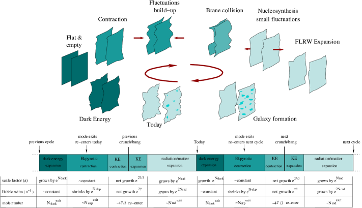
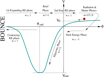
The cyclic333For a historical account of cyclic oscillating models dating back to the 1920’s see Kragh (2013). scenario is an extension of the old ekpyrotic scenario. It can, as the previous scenario, be described by means of an effective 4d scalar field whose potential is represented schematically on Fig. 2. It was introduced in Steinhardt and Turok (2002, 2001); Khoury et al. (2002a) and critized in Felder et al. (2002); Linde (2008). This cyclic extension with a singular bounce continues to be investigated. The idea is that after the brane collision, the inter-brane distance grows again, but since the branes continue to attract each other, the distance between them reaches an apex, before turning around. This quasi-static phase of the internal space is associated with the late time FLRW Universe of dark energy domination and flattens out the branes. Ultimately, the branes’ attraction wins and a new ekpyrotic phase takes place.
In this model, the current dark energy dominated Universe will be superseded by a contracting ekpyrotic phase, followed by a bounce, an expansion phase, and a subsequent phase of radiation and matter domination, succeeded by another dark energy dominated phase and continuing so in a cyclic manner. Fig. 1 shows a schematic representation of the cyclic model based on colliding branes in M-theory. A conceptual advantage of this model is the apparent lack of need for a specified microphysical origin of time, making the problem of initial conditions inconsequential, see Sec. III.1.5 for details and Table 1 for general properties of singular bouncing models.
However, it should be noted that the cyclic universe is not past eternal, similar in that regard to eternal inflation Mithani and Vilenkin (2012). Unfortunately, each singular bounce requires the use of non-perturbative techniques in string theory and is therefore ill-understood, if at all.
The spectrum of curvature fluctuations in the old ekpyrotic scenario was found to be deeply blue Brandenberger and Finelli (2001); Lyth (2002a); Durrer and Vernizzi (2002); Creminelli et al. (2005) (an additional problem is that these modes do not become classical Tseng (2013) as opposed to the ones resulting from the entropic mechanism Battarra and Lehners (2014) described below). As a result, two-field models Notari and Riotto (2002) were introduced to overcome this problem Lehners et al. (2007a); Buchbinder et al. (2007a); Creminelli and Senatore (2007); Buchbinder et al. (2007b). One realization is the new ekpyrotic scenario, a nonsingular setup, which makes use of the entropic mechanism to generate a nearly scale-invariant spectrum of primordial density fluctuations in an isocurvature field. If seen as a fundamental theory, the ghost condensate employed in the new Ekpyrotic scenario contains ghosts due to the higher derivative equations of motion, as shown in Kallosh et al. (2008). However, from an effective field theory (EFT) point of view, ghosts are absent below the energy scale demarcating the validity range of the EFT Woodard (2007). Thus, the description in the new ekpyrotic scenario is self-consistent, as long as the energy scale during the bounce remains below that cut-off, such that the degrees of freedom associated with the higher derivatives do not get excited.
| Instabilities | ||||||||||
|---|---|---|---|---|---|---|---|---|---|---|
| Model | Bounce | no tuned i.c. | no ghosts | A | B | C | D | |||
| Ekpyrotic Khoury et al. (2002b) | singular brane | ✗ | ✓ | ✓ | ✓ | ✓ | ✓ | blue Khoury et al. (2002b) | ? | |
| Cyclic Steinhardt and Turok (2001, 2002) | quant.grav.eff. | ✗ | ✓ | ✓ | ✓ | ✓ | ✓ | HZ | ? | |
| Phœnix Lehners and Steinhardt (2009) | brane collision | ✓ | ✓ | ✓ | ✓ | ✓ | ✓ | HZ | Lehners (2011a) | |
| Bars et al. Bars et al. (2011); Bars (2011); Bars et al. (2012, 2014a, 2013); Bars (2012); Bars et al. (2014b) | antigravity | ? | ✓ | ✓ | ✓ | ✓ | ✓ | ? | ? | |
A similar extension of the singular cyclic model to a two-field setup is given in Lehners et al. (2007a), which subsequently led to the proposal of the Phœnix universe Lehners and Steinhardt (2013); Lehners et al. (2009); Lehners (2011b); Johnson and Lehners (2012). The conversion from isocurvature to adiabatic modes, first proposed in Notari and Riotto (2002) to counter the problems encountered in the old ekpyrotic scenario444An idea taken from the curvaton mechanism Enqvist and Sloth (2002); Lyth and Wands (2002), which utilizes isocurvature perturbations to that effect., can occur before the bounce via the movement of fields away from the scaling solution towards an ekpyrotic attractor Koyama et al. (2007a); Koyama and Wands (2007); Koyama et al. (2007b) see also Buchbinder et al. (2007b) and Sec. IV.5.1 for details. Alternatively, a reflection of fields from a sharp boundary of field space can result in a different conversion Lehners et al. (2007b, c), see Sec. IV.5.2; one may also use the curvaton mechanism or modulated (p)reheating Enqvist and Sloth (2002); Lyth and Wands (2002); Battefeld (2008) after the bounce, Sec. IV.5.3. These entropic mechanisms are constrained by PLANCK Ade et al. (2014b, 2013b) due to their generic prediction of large non-Gaussianities. In that regard, it should be noted that different aspects are highlighted in the literature: before the improved constraints by PLANCK, Lehners et al. Lehners and Steinhardt (2008a, b); Lehners (2010) highlighted the generic prediction of observably large non-Gaussianities of of order or bigger for the conversion mechanism in Lehners et al. (2007b, c). However, after the publication of PLANCK, the emphasis was put onto the possibility to counterbalance different contributions to non-Gaussianities to enable of order Lehners and Steinhardt (2013). To this end, the focus shifted to potentials approximately symmetric transverse to the adiabatic direction, as well as non-minimal entropic models Qiu et al. (2013); Li (2013); Fertig et al. (2014); Ijjas et al. (2014b). All these models entail an unobservable primordial gravitational wave spectrum; they are therefore ruled out if the BICEP2 detection of is confirmed to be a signal of primordial origin by the future Keck Array observations at GHZ and PLANCK observations at higher frequency Flauger et al. (2014); Mortonson and Seljak (2014), see Sec. IV.3.
In a recent publication applicable to singular models Xue and Belbruno (2014), Xue et al. studied the classical dynamics of the universe experiencing a transition from a contracting phase, which is dominated by a scalar field with a time-varying equation of state parameter, to an expanding one through a big bang singularity. It was found that the evolution of a bouncing universe through such a singularity lacks a continuous classical limit except when the equation of state is highly fine-tuned; this result implies that a transition from contraction to expansion is contingent on quantum processes and not on a simple classical limit.
Other studies pertaining to the cylic universe, which are not reviewed here, include: 5D dynamics of general braneworld models Saridakis (2009), past-shrinking cycles that spend more time in an entropy conserving Hagedorn phase Biswas (2008), a cyclic magnetic universe Novello et al. (2009); Medeiros (2012), phantom accretion onto black holes Sun (2008), deformed Hořava-Lifshitz gravity Son and Kim (2011), a string-inspired model via a scalar-tachyon coupling and a contribution from curvature in a closed universe Li et al. (2014), cosmological hysteresis Sahni and Toporensky (2012), Finsler-like gravity theories constructed on tangent bundles to Lorentz manifolds Stavrinos and Vacaru (2013), a combination of cyclic and inflationary phases with quintessence Ivanov and Prodanov (2012) and a cyclic model with a chameleon field Gao et al. (2014a), among others Barrow et al. (2004); Clifton and Barrow (2007); Barrow and Sloan (2013).
II.3 String gas cosmology
The presence of a maximal temperature in string theory, the Hagedorn temperature, as well as T-duality led to the hope of constructing a nonsingular cosmological setup by invoking these intrinsically stringy phenomena Brandenberger and Vafa (1989); Tseytlin and Vafa (1992); Alexander et al. (2000); Kripfganz and Perlt (1988); Brandenberger (2005). Early work on string thermodynamics can be found in Hagedorn (1965); Frautschi (1971); Bowick and Wijewardhana (1985); Sundborg (1985); Alvarez (1986); Polchinski (1986); Salomonson and Skagerstam (1986); Mitchell and Turok (1987); O’Brien and Tan (1987). As the Hagedorn temperature is approached, new massless degrees of freedom arise, indicating a phase transition. This thermal component can be modeled by a string gas Brandenberger et al. (2013). String gas cosmology is an attempt to incorporate strings and branes into a cosmological setting by means of a gas approximation, see Battefeld and Watson (2006); Brandenberger (2008) for reviews. While attempts to construct alternative proposals to inflation in string gas cosmology, such as in Brandenberger et al. (2007a), are still subject to unsolved problems555Although it is possible to generate a nearly scale-invariant spectrum and gravitational waves, this proposals is still hampered by the flatness and relic problems; this is discussed in Sec. III.1.4. Battefeld and Watson (2004, 2006); Kaloper and Watson (2008), it was shown in a series of recent articles Florakis et al. (2011); Kounnas et al. (2012a, b); Kounnas and Toumbas (2013) that a string gas can be used successfully to describe the matter content in a Hagedorn phase, while providing the possibility of violating the NEC in a controlled manner in string theory. Based on this idea, a cosmological model has been constructed and cosmological perturbations were computed in Brandenberger et al. (2013). There it was shown that a nearly scale-invariant spectrum can be transferred through this nonsingular bounce, if it has been previously generated. The violation of the NEC mediated by an S-brane is under computational control and most instabilities can be avoided, with the notable exception of the Belinsky, Khalatnikov and Lifshitz (BKL) instability, see Sec. III.2.2; the model, dubbed S-brane bounce in this review, provides a promising avenue for future research. We discuss its ingredients in more detail in Sec. III.3.5.
II.4 A nonsingular bounce in string theory
An attempt to circumvent the initial singularity using methods akin to the AdS/CFT correspondence Maldacena (1998) was proposed in Turok et al. (2007) following prior work in Hertog and Horowitz (2004). The AdS/CFT correspondence provides a non-perturbative definition of string theory in anti de Sitter (AdS) spacetimes in terms of conformal field theories (CFT) Maldacena (2003a). In Turok et al. (2007) Turok et al. suggest the possibility of not only attaining a healthy nonsingular bounce, but also propose a new mechanism for generating nearly scale-invariant cosmological perturbations Craps et al. (2012). The cosmological set-up considered in Craps et al. (2012) is a toy model and not compatible with the necessary ingredients for the ekpyrotic scenario to take place. This line of research was subsequently followed in Craps et al. (2009); Smolkin and Turok (2012). At the time of writing, a cosmological model ready to be compared with observations has not been constructed.
II.5 Antigravity
In a series of papers, Bars et al. Bars et al. (2011); Bars (2011); Bars et al. (2012, 2014a, 2013); Bars (2012); Bars et al. (2014b) showed that theories motivated by the minimal conformal extension of the standard model with scalar fields coupled to gravity can be lifted to a Weyl-invariant theory that allows the cosmological evolution to be unambiguously traced through a big-crunch/big-bang (singular) transition. Here the classical evolution can be followed in a homogeneous, but potentially anisotropic (e.g. Bianchi IX), universe through a brief antigravity phase. Early work on antigravity can be found in Linde (1979). As pointed out in Carrasco et al. (2014); Linde (2014) and acknowledged in Bars et al. (2014b), this Weyl-invariant extension does not resolve the singularity: for example, the Weyl-invariant curvature squared diverges Carrasco et al. (2014); Kallosh and Linde (2014). Because of the presence of a curvature singularity, the use of classical General Relativity methods throughout Bars et al. (2014b) is therefore questionable.
Bars et al. argue that a geodesically complete, unambiguous solution arises, because the cosmic evolution becomes smoothly ultra-local so that density perturbations and spatial gradients become negligible Linde (2014). The presence of an unambiguous classical evolution through said singularity is intriguing and warrants further study666A resolution of cosmological singularities has been attempted in string theory repeatedly Cornalba and Costa (2002); Liu et al. (2002); Horowitz and Polchinski (2002); Cornalba and Costa (2004); Berkooz and Reichmann (2007) and is currently an active field of research., since it is unknown, at the time of writing, whether or not quantum gravity corrections leave the smooth transition found in Bars (2011); Bars et al. (2012, 2014a, 2013) unaffected. A debate on this topic can be found in Ijjas et al. (2014a); Linde (2014), and in particular it was found in Carrasco et al. (2014) that the curvature invariants diverge. If it can be shown that the considered Weyl-invariant quantities remain unscathed, one can employ this type of bounce in the cyclic scenario in lieu of the complicated ghost condensate/galileon models that we focus on subsequently in this review. Most recently, Oltean and Brandenberger (2014) considered two scalar fields, the dilaton and the Higgs, coupled to Einstein gravity and showed that the isotropic cosmological solutions deep in the antigravity regime are stable at the level of scalar perturbations Oltean and Brandenberger (2014). A full analysis is still an open research topic.
| P. inv. vac. | Instabilities | ||||||||
|---|---|---|---|---|---|---|---|---|---|
| Model | Bounce | sublum. | BKL | A | B | C | D | ||
| New ekpyrotic Buchbinder et al. (2007a); Khoury et al. (2002b) | ghost cond. | ✗ | ✓ | ✗ | ✗ | ✗ | ✗ | HZ | Koyama et al. (2007b); Buchbinder et al. (2008) |
| Matter bounce Brandenberger (2012); Cai et al. (2012a, 2013a, 2013b) | ghost.cond/gal. | ? | ✓ | ✓ | ✓ | ✓ | ✓ | HZ | Cai et al. (2009a) |
| G-bounce Easson et al. (2011) | KGB/galileons | ? | ✓ | ✓ | ✓ | ✓ | ✓ | blue | ? |
| Non-min entr. Qiu et al. (2013); Li (2013) | galileon/other | ? | ✓ | ✓ | ✓ | ✓ | ✓ | red | Fertig et al. (2014); Ijjas et al. (2014b) |
| Cosm. super-bounce Koehn et al. (2014) | ghost.cond/gal. | ✓ | ✓ | ✓ | ✓ | ✓ | ✓ | ? | ? |
| S-brane bounce Brandenberger et al. (2013) | S-brane | ✓ | ✗ | ✓ | ✓ | ✓ | ✓ | HZ | ? |
II.6 Nonsingular bounces via a galileon
Nonsingular scenarios often include a combination of a contracting matter dominated phase (ordinary dust or mimicked by a scalar field) to yield a nearly scale-invariant power spectrum, an ekpyrotic phase to dilute the curvature and shear contributions, followed by a bounce phase777 An exception is the new ekpyrotic scenario, which is nonsingular and does not contain a contracting, matter dominated phase. . Almost all of the hitherto mentioned bounce mechanisms have problems, such as the growth of instabilities and the presence of ghosts. In this section, we provide an overview of mechanisms based on galileon fields: these non-canonical scalar fields can induce a bounce while preserving the smooth, flat conditions achieved during the contracting phase and avoiding instabilities. They can further be implemented in supergravity and therefore provide a promising avenue for future research.
Galileon models Nicolis et al. (2009) arise naturally in the context of massive gravity de Rham and Gabadadze (2010); de Rham et al. (2011). These theories and their generalizations de Rham and Tolley (2010); Deffayet et al. (2010a); Kobayashi et al. (2010); Deffayet et al. (2010b) offer the intriguing option to start the cosmological evolution from a nearly Minkowski space-time to a de Sitter-like expansion Creminelli et al. (2010); Creminelli et al. (2013a), thus alleviating the initial value problem of inflationary cosmology. We would like to add, at this point, that the naturalness or unnaturalness of a set of initial conditions, e.g. starting with an empty flat universe, depends on a particular researcher’s viewpoint and is thus subjective.
Besides enabling inflationary models, a bounce can be induced via a galileon field Nicolis et al. (2009); Creminelli et al. (2010); Creminelli et al. (2013a) or its close relative, a field with kinetic gravity braiding (KGB) Deffayet et al. (2010a); Kobayashi et al. (2010). These models make use of a subclass of scalar field theories with higher order derivatives in the action while maintaining second order equations of motion, as classified by Horndeski Horndeski (1974). Galileon Lagrangians obey a symmetry under the Galilei transformation
| (11) |
where and are constants888In the literature, the galileon is often denoted by , a notation we shall not use here as the fields used in the literature on bouncing cosmology are commonly denoted ; here, we keep the latter notation.. See Deffayet and Steer (2013) for a recent review of the mathematical properties and construction of galileon theories. The Lagrangian of these types of fields can lead to NEC violation while avoiding instabilities and ghosts.
Consequently, bouncing cosmological models have been put forward using galileon fields, e.g. the G-bounce in Qiu et al. (2011); Osipov and Rubakov (2013) and Easson et al. (2011) (a follow up to KGB models) among others Deffayet et al. (2010a); Pujolas et al. (2011); Qiu (2014). A common danger of these models is the possibility of pressure/big rip singularities Barrow (2004), which are indeed present in the far past or future of a G-bounce Easson et al. (2011).
In Qiu et al. (2013), a nonsingular bounce in the framework of galileon cosmology with an ekpyrotic phase was investigated, with the addition of a curvaton instead of a matter phase to generate the scale-invariant spectrum of perturbations. This work superseded that of Li (2013) which set up the building blocks to obtain scale-invariant entropy perturbations within the ekpyrotic scenario via non-minimally coupled massless scalar fields. There, it was suggested that the entropy perturbation could be converted into curvature perturbations by means of a curvaton, as done in Qiu et al. (2013), or modulated (p)reheating Battefeld and Brandenberger (2004). Non-Gaussianities for the model in Qiu et al. (2013) where computed in Fertig et al. (2014), see the non-minimal entropic mechanism in Table 2. This model does not entail intrinsic non-Gaussianities, but the ones arising from the conversion mechanism. This particular model is an example of a more general class of non-minimal ekpyrotic models studied in Ijjas et al. (2014b).
A first attempt to implement galileons in supergravity turned out to be problematic, since the bosonic sector of globally supersymmetric extensions of the cubic Langrangian showed a reappearance of ghosts Koehn et al. (2013a); nevertheless, a follow-up study in Koehn et al. (2014) proved more successful: the necessary conditions for a nonsingular, stable, cosmic bounce in supergravity, and hence potentially allowed in string theory, are derived in Koehn et al. (2014); this so-called super bounce, see Sec. III.3.4, is based on supergravity versions of the ghost condensate and cubic galileon scalar field theories that have been used at the phenomenological level in the matter bounce scenario Cai et al. (2012a). This bounce is free of most problems that hamper many other nonsingular bounces, see Sec. V and table 2. It is therefore one of the most promising proposals.
II.7 Massive gravity
The idea of modifying gravity is not new. In 1939, Fierz and Pauli raised the question of the existence of a consistent covariant theory for massive gravity, whereby the graviton becomes massive, hence leading to a modification of General Relativity Fierz and Pauli (1939). However, the non-linear terms that curtail the discontinuity problem van Dam and Veltman (1970); Zakharov (1970), give rise to the Boulware-Deser (BD) ghost mode Boulware and Deser (1972). The prevalence of ghosts made the theory unstable and it was abandoned for decades until de Rham et al. constructed a non linear extension de Rham and Gabadadze (2010); de Rham et al. (2011): the ghost could be removed in the decoupling limit to all orders of perturbation theory through a systematic construction of a covariant non-linear action. It was soon realized, however, that homogeneous and isotropic solutions in non-linear massive gravity have a ghost De Felice et al. (2012, 2013). Extensions of non-linear gravity models ensued D’Amico et al. (2011); Gumrukcuoglu et al. (2012) and the graviton mass was allowed to vary by setting its mass via a scalar field Huang et al. (2012). Motivated by this work, the cosmological implications in flat and open universes were explored in Saridakis (2013); it was found that such an extension requires a UV-modification of General Relativity, in addition to the one in the IR. A pedagogical review of massive gravity can be found in Hinterbichler (2012) (see also de Rham (2014)).
Nonsingular bouncing cosmologies have been constructed within massive gravity. An attempt to construct ghost and asymptotically free modified gravity models that enable nonsingular bouncing solutions and resemble General Relativity in the IR limit was made in Biswas et al. (2006, 2010). Using the results of Saridakis (2013), where the graviton was promoted to a function of an extra degree of freedom, a nonsingular bounce and cyclic cosmological evolutions at early times were studied in Cai et al. (2012b); in Langlois and Naruko (2013), bouncing cosmologies were found to be generic in the context of massive gravity on de Sitter; the bounce occurs while the cosmological matter satisfies the strong energy condition. Other work include Biswas et al. (2012a, b) and Koshelev (2013a).
These models can provide a ghost-free bounce, but further implications have not been explored.
II.8 A nonsingular bounce in the multiverse?
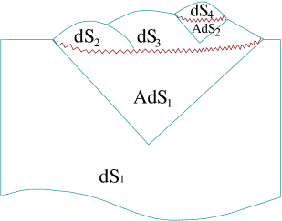
Attempts have been made to connect bouncing cosmologies to the inflationary multiverse. The latter is made up of different space-time regions populated by different meta-stable vacua. A transition from one vacuum to the next may occur via quantum tunneling, generating a daughter vacuum which expands within the parental one. Evolution after the tunneling depends on whether the vacuum inside a bubble has positive energy density or not. In the former case, the evolution is asymptotically de Sitter (dS) and further nucleation occurs within the bubble, the latter’s AdS vacuum (a contracting universe with negative cosmological constant) eventually collapses into a big crunch, developing curvature singularities where space-time ends999 See Lehners (2012) for populating different vacua in eternal inflation and the possibility to encounter emergent or even cyclic universes in the nucleated bubbles. It should be noted that any quantification of such ideas is dependent on the measure. . Such bubbles are called terminal. It has been speculated that the terminal singularity of the AdS vacuum is resolved in a complete theory of quantum gravity, such as string theory – see Fig. 3 for a causal diagram. In the absence of such a resolution, a phenomenological model yielding a nonsingular bounce based on the introduction of a term into the Friedmann equations, as in Sec. II.1.1, has been used in Garriga et al. (2013); Gupt and Singh (2014). In this study and in related works Piao (2004, 2009); Liu and Piao (2014), the transition between vacua during contraction and re-expansion was computed. Putting aside the theoretical shortcomings of the model used to replace the big crunch by a nonsingular bounce, the results of this work are of interest: if the vacuum is AdS () subsequent bounces take place until the field eventually emerges in a de Sitter vacuum. During these transitions, the field usually jumps a large distance of order in field space. Hence, at least at the phenomenological level, the AdS bounces may lead to transitions to remote parts of the landscape, reaching regions otherwise inaccessible. However, tachyonic instability and parametric resonance amplify scalar field fluctuations within the AdS bubble, albeit less efficiently than in slow roll inflation. If the fluctuations remain small, the whole bubble transitions to a similarly smooth vacuum; on the other hand, if fluctuations become large, the bubble volume fragments into different final vacua after the bounce. Transitions from one AdS vacuum to another one lead to further amplification, enhancing the probability of bubble fragmentation. This is reminiscent to models of eternal inflation discussed in Johnson and Lehners (2012). Bubble wall fluctuations can give rise to strong anisotropies in the contracting AdS bubble, leading to BKL instabilities and Kasner periods, see Sec. III.2.2, with the eventuality of further bubble fragmentation. In Liu and Piao (2014), it was found that bubbles fragment within two or three transitions based on the enhancement of field perturbations induced by the amplification of curvature perturbations. In a follow up study Vilenkin and Zhang (2014) it was shown that even in the presence of AdS bounces, space-time is still past-incomplete as in inflationary cosmology. Thus the initial singularity is not resolved, but merely pushed out of sight and hence, as in the corresponding inflationary framework, physically inconsequential.
II.9 Other models
The models presented above represent the mainstream ideas that have been proposed to implement a bouncing alternative to inflation. We conclude this general model presentation by identifying some miscellaneous proposals Novello and Bergliaffa (2008), which are generally viewed as less fashionable and/or are hampered by conceptual problems.
II.9.1 Hořava-Lifshitz
Hořava-Liftshitz (HL) gravity, first introduced in Horava (2009a), is a power-counting renormalizable theory of gravity with purportedly consistent UV-behavior and a fixed point in the IR-limit Horava (2009b, c). Therefore, as a modification to General Relativity at high energies, this theory was explored significantly within the context of cosmology: cosmological solutions with matter and the possibility of a nonsingular bounce were studied in Calcagni (2009); Kiritsis and Kofinas (2009); Brandenberger (2009); Maier (2013). HL gravity was shown to have inconsistencies in Henneaux et al. (2010) and more recently, to be UV-incomplete Kimpton and Padilla (2013). We therefore do not dwell on these models further.
II.9.2 Lee-Wick and Quintom
Lee and Wick Lee and Wick (1969, 1970) proposed, in the late sixties, a finite version of QED; based upon this proposition, Grinstein et al. constructed a modification to the standard model known as the Lee-Wick Standard Model Grinstein et al. (2008); this model aspires to provide an alternative to supersymmetry. A feature of these models is the presence of phantom fields Caldwell (2002). Phantom fields have several conceptual problems Cline et al. (2004) since the equation of state parameter is less than , but they might enable a bounce. In addition, a future singularity is present and the vacuum is unstable. Despite these problems, Lee-Wick theory continues to be investigated and several nonsingular bouncing models have been constructed within its framework. For instance, a nonsingular bounce caused by a Lee-Wick type scalar field theory was studied in Cai et al. (2009b) providing a realization of the matter bounce scenario; the authors found a scale-invariant spectrum for both scalar perturbations and gravitational waves, in agreement with Allen and Wands (2004), see Sec. IV.2.4. See Bhattacharya et al. (2013) for a follow up study.
Quintom models (two matter fields, one regular, the other with a wrong sign kinetic term to violate the NEC Feng et al. (2005), see Brandenberger (2012) for a review) alleviate the problem of a future singularity, leading to a proposal of a quintom bounce Feng et al. (2005, 2006); Guo et al. (2005); Cai et al. (2008, 2007).
Besides providing a nonsingular realization of a bounce, which is hampered by the conceptual problems of Lee-Wick theory, these models do not provide any additional desirable features; we shall therefore not consider them any longer. It should however be acknowledged that the techniques developed for studying perturbations and extracting observables in these toy models served as a stepping stone towards the development of healthier scenarios such as galileon bounces in supergravity, discussed in Sec. II.6.
II.9.3 , and Gauss-Bonnet gravity
Most of the models developed above imply modifying gravity in one way or another, yet they do not include the simplest such possibility, namely that for which the Einstein-Hilbert Lagrangian is replaced by an arbitrary function of the Ricci scalar De Felice and Tsujikawa (2010). Assuming a flat FLRW metric, one can reconstruct the function that would be required to produce a given bouncing behavior for the scale factor Bamba et al. (2013). In this context, dark energy models incorporating a bounce were constructed in Astashenok (2014) and the interaction between dark energy and dark matter was studied in Brevik et al. (2014); it turns out that a Gaussian bounce, with scale factor behaving as , occurs only in the unphysical region with and , hence leading to an instability with respect to the production of tensor perturbations. On the other hand, a power law bounce () can take place with simple monomial forms of , in the stability region. In addition, the latter models can be smoothly connected to more common contracting and expanding phases.
A similar construction, leading to a bouncing phase connecting two respectively contracting and expanding de Sitter phases, can also be performed, yielding a possible oscillatory signal in the spectrum of gravitational waves Bouhmadi-Lopez et al. (2013). In this case, the mass of the associated scalar field can become negative close to the bounce, leading to instabilities, which manifest themselves in the ensuing spectrum.
The same technique of Lagrangian reconstruction can be used assuming a function of the Gauss-Bonnet invariant instead of one of the curvature Ricci scalar . Bouncing solutions were explored in Bamba et al. (2014), some of which were found to be stable.
Instead of choosing an arbitrary function of the Gauss-Bonnet term, one can also consider a non local extension whereby an analytic but otherwise arbitrary function of the D’Alembertian operator is inserted in between the non-linear terms; for instance . This procedure naturally introduces a new energy scale and the new terms behave in the FLRW case as effectively negative energy fluids. Because such terms are essentially non local, perturbations are difficult to implement, but some arguments have been presented that suggest these solutions to be stable Koshelev (2013b).
Instead of using the curvature scalar as the basic ingredient to build the action by means of the torsionless Levi-Cività connection, one can also use the curvatureless Weitzenböck connection constructed from the vierbein , the metric , and the local Minkowski metric . This yields the so-called “teleparallel” Lagrangian Hayashi and Shirafuji (1979), which is nothing else but the torsion scalar , which provides a different, yet equivalent, formulation of GR. Adding an arbitrary function of the torsion provides a natural extension, which has been investigated recently in view of explaining the observed acceleration of the Universe Linder (2010). An advantage of models over ones is that their equations of motion remain second order, and therefore reduce the risk of instabilities. The gravitational part of such models can effectively violate the NEC, thus implying possible bouncing solutions, even for vanishing spatial curvature Cai et al. (2011a). The procedure, however, requires special forms of the otherwise arbitrary function .
The spectrum of perturbations predicted in the expanding phase for the models detailed above, and hence their compatibility with the data, is unknown.
II.9.4 Brane worlds and extra-dimensions
String theory can be made mathematically self-consistent provide spacetime has more than 4 dimensions, the extra dimensions being usually assumed to be internal and small. Branes are extended objects in this framework, which can move in those internal dimensions. The corresponding 4D-effective field theories can be sufficiently rich to enable a bounce. For example, the ekpyrotic scenario, as originally envisioned, can be seen as an example of a brane-world set-up, see Sec. II.2.
The Gauss-Bonnet action, although non-dynamical in 4 dimensions, can also be obtained in the low energy limit of heterotic superstring theory and studied in any other number of dimensions. Thus, such a term is well suited to investigate brane-world scenarios: in Maeda (2012), a 4 dimensional brane, on which a perfect fluid with constant equation of state evolves, is embedded in a 5 dimensional Randall-Sundrum Randall and Sundrum (1999) like setting. The conditions are derived under which the brane scale factor can bounce. A branch singularity, actually a real curvature singularity, exists at a finite physical radius in the bulk: when the brane encounters this singularity, its scale factor instantaneously bounces from a contracting to an expanding phase; there is no telling as to what will happen with perturbations.
A bouncing solution was also found in the case in which the D3-brane is the boundary of a 5 dimensional charged anti-de Sitter black hole Mukherji and Peloso (2002): it is the charge which provides the negative energy regularizing term in the effective 4D Friedmann equation, and thus permits the avoidance of the singularity through a bouncing phase. On the 4D brane, this charge behaves as a stiff matter fluid, .
Relevant for the ekpyrotic scenario is the study in Turok et al. (2004), which provides a semiclassical treatment of the collision between two empty orbifold planes that approach each other at constant speed. In this toy model, it is shown that the big crunch/big bang transition appears smooth in the sense that certain states can propagate smoothly across the transition. It is further argued that interactions should be well-behaved since the string coupling approaches zero during the transition. However, a realistic transition remains an active field of research.
Conceptually unrelated to brane-world scenarios in string theory, one may entertain the idea of extra timelike dimensions. These might pose conceptual questions, as it is not clear at the time of writing if they are compatible with causality, if they predict tachyonic modes and/or if they entail negative norm-states as is sometimes argued. Ignoring these questions for the time being, it is possible to construct bouncing cosmologies in this new framework. Considering a Randall-Sundrum-like scenario with an extra timelike dimension instead of a spacelike one, the effective energy momentum tensor contains a term proportional to , which enables the transition from contraction to expansion at high energies Shtanov and Sahni (2003); Brown et al. (2008). While these theories differ from Randall-Sundrum models by merely a sign, they have never been implemented in string theory. Cosmological perturbations were studied in Battefeld and Geshnizjani (2006); Geshnizjani et al. (2006), where it was found that a scale-invariant spectrum can survive such a particular nonsingular bounce, if it is generated in the preceding contracting phase. Since the term quadratic in the energy momentum tensor does not add additional degrees of freedom at the perturbed level, one cannot apply the results derived in two field models, as in Bozza and Veneziano (2005).
II.9.5 Non relativistic quantum gravity
There are theoretical frameworks in which LI is not necessarily fundamental but might instead arise as an emergent property of space-time. Such an approach permits theories in which this symmetry is not implemented from the start, opening the possibility to quantize the spatial degrees of freedom independently, and leading to a non-relativistic quantization of gravity. Since Lorentz invariance is an extremely well-tested symmetry of nature, see Sec. II.1.1, and an integral part of high energy physics and string theory, it is often challenging to reconcile such proposals with observations. Ignoring these conceptual pitfalls, one may try to construct bouncing cosmologies under these conditions.
Effective field theory within such frameworks allows up to 6th order spatial derivatives in the action, which can contain all scalar combinations of the tensors and (together with some matter contribution). Restricting attention to the FLRW metric, Cai et al. Cai and Saridakis (2009), find a dark radiation term with negative energy density in the Friedmann equations, provided that the spatial sections are not flat. Thus, bouncing and even cyclic solutions, can be obtained. Incorporating a matter-dominated contracting phase, perturbations have been found to possibly induce a slightly red tilt in the spectrum, although the cyclic continuation may generate backreaction problems.
II.9.6 Mimetic matter
The mimetic matter model Chamseddine and Mukhanov (2013) mimics a phantom field by introducing an auxiliary metric and a scalar field in terms of which the actual metric reads ; this happens to be equivalent to a dark matter component, the scalar field being not entirely dynamical because of the normalization condition . The action is given by the Ricci scalar of and contains just one extra longitudinal degree of freedom. It can be supplemented by an arbitrary potential . If the FLRW background metric is used, the scalar field becomes a function of time, leaving the potential to behave in the Friedmann equations as another arbitrary function of time. Choosing for instance leads to bouncing solutions Chamseddine et al. (2014). However, because of the non dynamical nature of the scalar field involved, canonical quantization is not always feasible and therefore setting initial conditions for perturbations can be impossible.
II.9.7 Nonlinear electromagnetic action
Before inflation was conceived, Novello et al. Novello and Salim (1979) proposed to implement a bounce in a cosmological framework, in which the matter content is provided by a massless vector field . These models rely on two categories of modifications of electromagnetism, i.e. models with non-standard coupling to gravity, using terms in the Lagrangian of the form , , , and models with scalar quantities similarly built out of the curvature and the electromagnetic tensors.
Extending electromagnetism to include nonlinear terms such as those in the Euler-Heisenberg corrections Heisenberg and Euler (1936) provides another option to generate a bounce: the action becomes an arbitrary function of the invariants and . Such terms are, however, usually only justified provided that the electromagnetic fields vary slowly compared to the electron length scale, but one can argue that similar terms should be obtained in the more general situation one is concerned with in the early stages of cosmological evolution.
By including a combination of such terms, the FLRW symmetry is kept by demanding either that some averaging procedure is applied to the electromagnetic field, or that the vector field has the special timelike structure . Bouncing solutions arise because the extra terms contribute negative quantities of energy density. Similar ideas were revisited to provide more general nonsingular solutions with either massless or massive vector fields sourcing gravity Artymowski and Lalak (2012).
The models described in this section and others are discussed in greater depth in Novello and Bergliaffa (2008). We shall not consider them further, since it is not clear whether they can actually be constructed self-consistently, i.e. without having insoluble intrinsic difficulties (ghosts, violation of causality, shear/vector mode overproduction, etc. ), and because their cosmological relevant consequences have not been established.
II.9.8 Spinors and torsion
A less known method of modifying gravity is provided by the Einstein-Cartan-Sciama-Kibble extension Kibble (1961); Sciama (1964), in which the affine connection is not necessarily symmetric, leaving the torsion tensor to behave as an independent dynamical variable. These new degrees of freedom couple only to spin densities and vanish outside material bodies, rendering them useless in most contexts. Since there is no exterior in cosmology, a fermionic field would induce an everywhere non-vanishing spin density, whose coupling to the torsion behaves as a NEC violating term in the Friedmann equations. This can generate bouncing solutions of a special kind, as the scale factor reaches a non-vanishing minimal value at a cusp, i.e. the Hubble rate is discontinuous at the bounce point Brechet et al. (2007, 2008); Popławski (2012). This raises serious questions regarding stability and the fate of perturbations.
A similar model, in which a topological sector is added to gravity, was proposed in which the bounce behaves in a more regular way; by adjusting the fermion number density and the mass, such a model can reproduce a scale-invariant spectrum of perturbations Alexander et al. (2014).
III Requirements for a successful bounce
In order to provide a viable alternative to inflation, a model should, at least, do as well as inflation in many respects. This implies that such a model’s cosmological predictions must not only be compatible with the currently available data, but also have a sound theoretical foundation. As we shall see, this is not an easy endeavor; before moving to these difficulties, we discuss the common puzzles of the standard hot big-bang model and their proposed solutions in bouncing scenarios.
III.1 Cosmological puzzles
Inflation was proposed as a way out of three observational conundrums: why is the universe isotropic on the largest accessible scales (the horizon problem)? Why does the content of the universe sum up in the exactly required fashion so as to make its spatial curvature negligible (the flatness problem)? Why do we not observe an absurdly large number of thermal relics, such as gravitinos in supersymmetric theories, or topological defects from phase transitions, such as primordial magnetic monopoles that should have been copiously produced during a grand unification transition (the relic problem)? Before we consider these questions, we would like to address a point that is often ignored in the literature on inflationary cosmology,that of the primordial singularity.
III.1.1 A primordial singularity?
Ever expanding cosmologies have been shown to be past incomplete Borde et al. (2003), so that, as far as classical gravity is concerned, the Universe began with an initial singularity. This problem, if one sees it as one, is not directly addressed in the inflationary framework: it is often postulated that the cosmological evolution begins in an epoch during which the relevant physical theories are well understood; previous phases are thought to be in the realm of quantum gravity and it is assumed that they have limited influence on the scales of observational relevance. Demanding that inflation “solves” the singularity problem would be similar to demanding that Big-Bang Nucleosynthesis (BBN) explains why the Universe was homogeneous and radiation dominated at the time it took place: it seems to us that one can make this hypothesis and assume some other physics to provide the necessary explanation without hampering the predictivity of BBN. Similarly, we think it is perfectly reasonable to assume that the primordial singularity is somehow resolved; an option would be to connect the currently expanding Universe to a previously contracting phase through a bounce. In this sense, studying bouncing solutions addresses an extremely relevant question ignored, or perhaps overlooked, in the inflationary paradigm.
III.1.2 Horizon problem
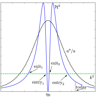
Big-bang cosmology provides a successful description of the evolution of the Universe back to a fraction of a second after its birth; it is consistent with the Hubble expansion, the cosmic background radiation and the abundance of light elements. Extrapolating to early times, we encounter what is called the horizon problem. The main assumption in big bang cosmology is large-scale homogeneity and isotropy. This assumption is in agreement with the cosmic microwave background radiation, whose temperature, if measured in two different, opposing patches of the sky, is the same to within at least one part in . Because the big bang contains an initial singularity, a causal horizon exists beyond which one should not expect similar thermodynamical properties. Based upon this fact, opposite patches in the sky could never have been in causal contact in the standard big bang model, and yet they have the same CMBR temperature to one part in .
The horizon size , during a radiation and matter dominated universe is of order when the origin of time is and the scale factor has power-law behavior for all times. At the time of last scattering the horizon size is Peter (2009)
| (12) |
where is the redshift of the last scattering surface; the angular diameter distance to this surface is
| (13) |
at the time of last scattering, so that the causal horizon size subtends an angle of
| (14) |
radians. For a redshift to the surface of last scattering, , we get . Thus, patches of the universe that were separated by more than this have no causal reason to have the same temperature. This is illustrated in Fig. 4.
In the big bang model, it is assumed that the universe was originally highly homogeneous and isotropic on scales larger than the causal horizon, indicating a high degree of fine-tuning. One might argue that such initial conditions make no sense in the framework of GR.
Inflation solves this puzzle by adding a phase during which the scale factor grows quasi-exponentially, in such a way that the causal horizon grows larger than any other physically relevant scale. The Hubble scale remains more or less constant, so the scale factor behaves roughly exponentially, , leading to an exponentially increasing horizon, i.e. , with the duration of the inflationary phase. It suffices that this duration be large enough, in practice , so that the resulting horizon scale is much larger than the entire observable Universe today. Moreover, a given quantum fluctuation of wavelength sourced in the far past can start out smaller than ; due to its subsequent growth , the wavelength becomes larger than , which remains roughly constant. Nevertheless, it remains within the causal horizon, which grows tremendously: no scale actually ever becomes “super-horizon”. This is necessary for any consideration in GR, including the setting of initial conditions, to make sense.
Bouncing models solve this puzzle in a completely different way. As far as the background is concerned, consider a contracting phase between and dominated by a perfect fluid with constant equation of state parameter , so that the scale factor behaves as ; we assume the bounce to take place at . The contribution of this contracting phase to the horizon is (we correct a misprint in Peter and Pinto-Neto (2008) from which the argument is taken)
| (15) |
which can be made arbitrarily large for provided that .
As for the perturbations, we consider that quantum fluctuations are sourced in the far past, deep within the horizon and the Hubble scale. The horizon itself grows at all times, and it is possible to have it growing more rapidly than the scale factor, so that a wavelength initially smaller than the horizon remains so at all subsequent times. During a slow contraction, the wave modes stay approximately constant, whereas the Hubble scale is rapidly shrinking as the bounce is approached; thus, modes which are sourced by quantum mechanical fluctuations inside the Hubble radius become super-Hubble during the contraction101010Colloquially, Hubble radius crossing of a particular mode is often referred to as “horizon” crossing, even though the Hubble radius is not a horizon in a contracting universe (and neither is it, as far as causality arguments are concerned, in an inflationary universe); we will not use this possibly confusing terminology Martin and Peter (2004a), particularly in view of the fact that both inflation and bouncing cosmologies are introduced in order to solve the horizon problem in such a way that the actual causal horizon becomes much larger than any relevant scale., but remain sub-horizon; thus a causal mechanism to seed the observed structures on large scales is present. The horizon problem is solved, because a lot more time is available to establish causal contact, see Fig. 5.
III.1.3 Flatness problem
The present density of the universe is close to the critical density, , where
| (16) |
with , and the relative energy densities of the cosmological constant, matter and radiation, respectively, while the dimensionless time-dependent curvature parameter is
| (17) |
Deviations from grow in time in a decelerating expanding universe. In order to have today, it must have been extremely close to one in the early universe, indicating fine-tuning. Data from the CMBR and Type Ia supernovae indicate that . Since
| (18) |
a non-accelerating expanding phase, such as one dominated by a radiation or a dust-like fluid, always increases ; hence, observing a small today requires fine-tuning of its initial value.
Specifically, the temperature of the universe dropped from about K at s to approximately K at s, the beginning of the matter dominated era; from then on up until today, the scale factor has been increasing as (we ignore the cosmological constant), so that the curvature parameter in (17) has also been increasing as . Thus, for today, it had to be less than at K. Furthermore, during the radiation dominated era, we have , so that , indicating that at K. That the value of this dimensionless parameter ought to be so small compared to unity in the early Universe is called the flatness problem Weinberg (2008).
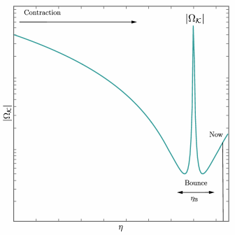
Inflation solves this problem in a simple way: consider (18) and add, for a sufficiently long period of time, a phase of accelerated () expansion (). In this case, and naturally evolves towards small values. To ensure that today, one needs roughly e-folds of inflation if initially. At the end of a quasi-exponential phase with , (18) indicates that , again requiring in order for the subsequent evolution of to be consistent with today’s upper bounds.
This problem is not solved in many alternative proposals to inflation: in string gas cosmology fine-tuning is required and in models akin to the original ekpyrotic proposal a vanishing is selected initially by symmetry arguments; for example, in the original ekpyrotic proposal the brane that we live on is a BPS brane Khoury et al. (2001a) (see however Kallosh et al. (2001b)). In the Phœnix universe, the currently accelerated epoch is used as a means of getting rid of the curvature term. In a way, the cyclic scenario may be seen as yet another (very low energy) implementation of the inflationary paradigm since in this model there are e-folds of cosmological constant domination before the contracting phase, making everything flat Linde (2014). In this sense, it can be argued that it is not really an alternative to inflation.
However, in a bouncing scenario, the flatness problem can be solved in an altogether different way: consider (18) in a decelerating () and contracting () universe. The curvature contribution can be made as small as desired during this contraction, as shown in Fig. 6. However, close to a nonsingular bounce, the curvature contribution grows again: consider the Friedmann equation (7) with the energy density of whatever matter happens to contribute at that time
the r.h.s containing terms behaving like (matter), (radiation) or even (shear), all of which dominate over the curvature term whenever the scale factor decreases (). Therefore, if the bounce takes place because of any term on the r.h.s., i.e. in the energy density , it may be that the curvature remains negligible at the expense of having a negative energy density source, thus potentially causing new instabilities.
Subsequently, grows large at the bounce, although it has to remain sufficiently small right after the bounce at the beginning of the expansion phase, so that it can still be negligible today. The amount of necessary “fine-tuning” is then transformed into a requirement that the bounce be sufficiently symmetric: if the curvature term was negligibly small at the end of the contracting epoch, it stays roughly negligible at the beginning of the expansion epoch. This fine tuning is exactly of the same nature as that found in inflation, which requires the accelerated expansion phase to last at least e-folds. In many bouncing models, the relevant amount of contraction is in far excess of the amount of expansion after the bounce until today. As a result, the flatness problem is solved as long as the bounce is sufficiently symmetric. This mechanism is illustrated in Fig. 6.
III.1.4 Avoidance of relics
Topological defects, exotic particles and even primordial black holes (PBH) can be created during the early stages of the Universe. Since estimates of the PBH production rate differ by many orders of magnitude, they are commonly ignored by model builders. The other kinds of relics must be considered carefully, since their production rates are well understood, once a model is specified. See Battefeld and Battefeld (2009a) for a brief review by one of the authors of this article and a collaborator, which we partly reproduce below.
Supersymmetric theories generically predict the existence of the gravitino, the supersymmetric partner of the graviton. The gravitino mass has its origins in spontaneous supersymmetry breaking and its value ranges from GeV to TeV. Since the gravitino is long-lived, if its dominant decay mode consists of a photon and its superpartner, it provides a natural candidate for dark matter. However, even in the absence of primordial gravitinos, they can be thermally produced during the radiation dominated epoch: this is an example of a thermal relic. The presence of thermally produced relics such as gravitinos imposes stringent constraints on the allowed maximal temperature in the radiation epoch. As a result, one finds an upper limit on the reheating temperature of order GeV. In any model of the early universe, be it inflation or a bounce, this constraint must be satisfied. Recall that supersymmetry is a key ingredient in string theory, so these relics are natural in this context. This problem can be alleviated by a second phase of reheating of a long-lived oscillating scalar. Examples of such fields are the s-axion in F-theory Heckman et al. (2010) or moduli in G2-MSSM models arising from M-theory compactifications Acharya et al. (2008), but a concrete implementation in bouncing cosmologies has not been given.
A different example of heavy relics spoiling the subsequent evolution of the Universe are super heavy magnetic monopoles as predicted in theories entailing grand unification (GUT): since the photon is a massless particle, we know for sure that at the current-day temperature of the Universe, the gauge group of particle physics contains a subgroup. Assuming a GUT based on a (semi)simple gauge group, , the presence of a factor in the resulting low-energy symmetry group implies that the second homotopy group of the vacuum manifold is non trivial, i.e. . As a result, stable solutions of the point-like kind (in 4D-spacetime) must form as topological configuration in the symmetry-breaking Higgs and gauge fields. With a symmetry breaking energy scale and a unification coupling constant , this mechanism produces objects whose mass can be estimated as Ringeval et al. (2007); Peter and Ringeval (2013); Ade et al. (2013a); Huguet and Peter (2000).
In the original hot big bang scenario, beginning with a singularity, at least one such monopole per horizon is produced during the GUT phase transition: this Kibble mechanism is due to causality, resulting in an over abundance of order today, if the universe cooled down from the GUT temperature of approximately GeV.
The inflationary solution is again simple and natural Guth (1981): the accelerated expansion dilutes all prior relics during inflation and as long as the reheating temperature is low enough, no further relics are produced. However, this problem resurfaces acutely, for instance, in the S-brane bounce, since a thermal component is present. Since (p)reheating has not been studied in bouncing cosmologies beyond simple estimates Lehners (2011b); Cai et al. (2011b), it is unknown at the time of writing whether or not thermal relics are formed111111 Inflationary and bouncing solutions differ fundamentally; in the former, the reheating temperature is bounded from above by the energy scale of inflation, whereas, in the latter it is not a priory bounded. In Lehners (2008), Lehners et al. envisioned reheating in the cylic scenario as occurring via the transfer of some kinetic energy between branes. Given this reasoning, it is possible to argue that the temperature can be expected to be below the upper limits quoted. Yet, the uncertainty of reheating dynamics in the cyclic scenario, and other bouncing models, is considerable greater than in inflationary cosmology. This is pointed out in more detail in Sec. VI.1. . Nevertheless, the defect question becomes a crucial one, not on considerations of energy density and relative contribution, but more fundamentally, because of the initial conditions they demand: if many Higgs fields are originally present in the large and cold universe, some of them must have vacuum expectation values, which in turns means, for most of those, arbitrary phases. As far as we know, there seems to be no natural and accepted way to set up these phases; further, it is not even clear if such mechanisms exist.121212 Although the phase issue may still be an open one, the monopole question can possibly be solved in a string theory context since the effective field theory which emerges as its low-energy limit is in general not based on a simply connected GUT group, so that the relevant symmetry-breaking scheme may not include monopole formation Polchinski (1998); Braun et al. (2006, 2013). .
III.1.5 Homogeneity and initial conditions: the Phœnix universe as a case study
Inflation initiates in a tiny region of space, assumed to be roughly homogeneous; this region expands to a huge size, thus effectively providing a mechanism to considerably alleviate (not solve), the problem of having a homogeneous Universe. Given that we observe homogeneity on sufficiently large scales, any alternative model should also yield an explanation at least as satisfying as that provided by inflation. In that respect, bouncing cosmology, with its contraction phase, can be in trouble.
A simple possibility considered by one of the authors of this review in Peter and Pinto-Neto (2008) consists in arguing that a large universe filled with diluted matter can be assumed to be initially roughly homogeneous, as it is mostly empty (although one should impose some extra constraints on the behavior of the Weyl tensor). Provided the contraction is sufficiently slow compared to the diffusion rate of the particles present at such early stages, one expects any initial inhomogeneity not only to remain small, but to be smoothed away through diffusion processes, thus dynamically driving the universe towards a homogeneous state of equilibrium. This method is, however, not necessarily stable w.r.t. the inclusion of a cosmological constant Maier et al. (2012).
Another option is employed in the cyclic model Steinhardt and Turok (2002), which traces back to Lemaître’s closed, oscillatory model of the universe undergoing repeated periods of big bang, expansion, contraction and big crunch Lemaitre (1997). Contrary to Lemaître’s model, the cyclic universe has an added component, a phase of ekpyrotic contraction Erickson et al. (2004); Garfinkle et al. (2008), that smoothens and flattens the universe. See Sec. III.2.1 and Lehners (2008) for a review. In accord with Lemaître’s model, the underlying idea of the original cyclic scenario is that the entire universe partakes in the cycling. Recycling the whole universe can be problematic if the entropy density grows from cycle to cycle, since our universe has low initial entropy; this problem can be avoided if the universe increases sufficiently from one cycle to the next, so that the entropy density does not grow. Nevertheless one still needs to understand how the first cycle came into being. Further, initial conditions appear to be extraordinarily fine-tuned in any model that uses the entropic mechanism to generate the scale-invariant spectrum131313See however the non-minimal entropic mechanism in Qiu et al. (2013); Li (2013); Fertig et al. (2014), which has a stable direction in the entropy direction..
To alleviate these problems, the Phœnix universe was proposed Lehners and Steinhardt (2009): the universe is reborn from a surviving seed found among its ashes, which goes hand in hand with generating curvature perturbations by means of the entropic mechanism Lehners et al. (2007a). See Sec. IV.5. Namely, due to the instability of the classical ekpyrotic trajectory along the potential to transverse fluctuations, large portions of the universe are converted into inhomogeneous remnants and black holes which are not able to pass through the cycles. Nevertheless, if a dark energy expansion phase with at least e-folds is present before the ekpyrotic contraction, a sufficiently large portion of space makes it down the classical trajectory and through the big bang; this patch grows from cycle to cycle. See Figs. 7 and 8. The dark energy expansion makes space smooth and flat; thus, this model seems to successfully address the question of flatness, fine-tuning at the background level and initial conditions for perturbations; in a way, such a model can be seen as a special implementation of the low-energy inflationary paradigm with an added curvaton mechanism to produce fluctuations, since the current-day accelerating phase has a pre-big bang counterpart one could dub inflationary.
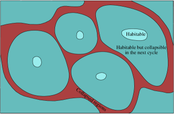
.
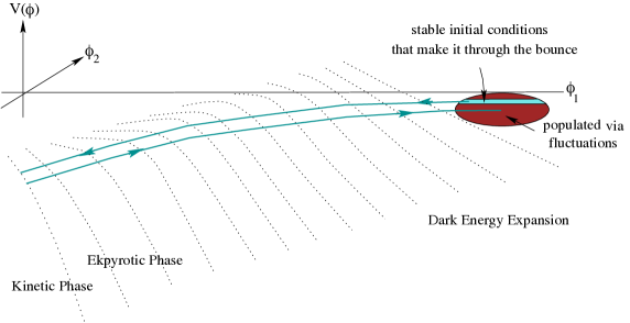
An important consequence of the Phœnix universe pertains to the amplitude of primordial density fluctuations Lehners and Steinhardt (2011), as parametrized by the so-called Mukhanov-Sasaki variable of the adiabatic mode , see (89) below. In contrast to inflation where is fitted by hand to be in agreement with observations, , in the cyclic model, patches of the universe with the appropriate value of are dynamically selected. This model employs an entropic mechanism and a change in the direction in which the scalar field moves after a turn in field space to convert isocurvature modes to adiabatic ones, see Sec. IV.5. According to this mechanism, all patches that make it through the bounce must have a value Lehners (2011b)
| (19) |
However appealing it might be, this model produces large amonts of non-Gaussianities that stem from the entropic mechanism Lehners (2011b) together with hardly any gravitational waves, see Sec. IV.3. It is thus in tension with current measurements Ade et al. (2014b, 2013b, 2013c).
It is interesting at this stage to mention a possible renewal of the solution to the cosmological constant problem proposed in Linde (1986) (see also another discussion of the same idea in Garriga et al. (2004)). L. Abbott proposed a more involved version of this idea Abbott (1988) which can be implemented in the cyclic model Steinhardt and Turok (2006); Lehners et al. (2009). The cosmological constant, , which is assumed to start out large and positive, steadily decreases to lower values via tunneling along a long stream of vacuum states, see Fig. 9 (this is not to be confused with other classes of scenarios for which the cosmological constant starts out large but is diminished by quantum gravity effects, thereby inducing either a phase of inflation or the current acceleration Romania et al. (2013)). After each successive tunneling event, the universe spends more and more time in the respective vacuum, because the value of the cosmological constant is lower than before, reducing the tunneling rate. The universe ends in a big crunch141414It has been speculated that transitions from AdS to dS may be possible during a bounce, leading to an implementation of bouncing cosmologies in the inflationary multiverse Garriga et al. (2013), see Sec. II.8. if the tunneling event leads to a negative value of . The presence of many habitable patches in the cyclic universe solves the cosmological constant problem à la Weinberg Weinberg (1989): after many cycles, any habitable patch sits in the lowest vacuum with . The problem of the original proposal by Abbott was that the tunneling events required eons to commence, so that any initial matter in the universe diluted, leading to an empty universe; the cyclic model circumvents this problem because a large matter density is produced during each cycle; hence the universe does not end up empty.
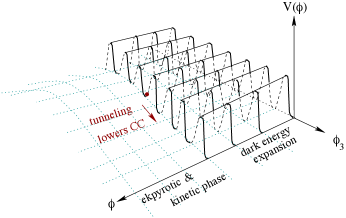
III.2 New challenges
Just like having a phase of inflation generates new challenges, such as the trans-Planckian problem Brandenberger and Martin (2013) or the measure problem, implementing a bounce gives rise to new issues. These belong to two categories: the first are cosmological in nature, for instance, a phase of contraction can lead to an unwanted increase of primordial shear; the second are of a theoretical kind, since in order for a bounce to be able to take place in GR (with flat spatial curvature), the underlying theory must be capable of violating the Null Energy Condition (NEC) without introducing instabilities.
III.2.1 The shear and the need for an ekpyrotic phase
In a contracting universe, anisotropies tend to grow, potentially spoiling the isotropy seen in the CMBR. Consider negligible initial curvature and a metric of the Bianchi I type, i.e.
| (20) |
with . The Einstein equations become
| (21) |
where , is the energy density contained in the anisotropy stemming from the functions (the shear) and
| (22) |
Eqs. (21) and (22), together with the fact that , imply that , and .
The FLRW limit, which is currently observed to be valid, must be recovered. At first sight, this seems to be impossible in a contracting phase: the continuity equation (8) for the constituents of the universe interacting exclusively via gravity with energy densities , pressure density and equation of state parameter is
| (23) |
and hence, each component, radiation (), non-relativistic matter (), cosmological constant (), curvature (), or shear density (), evolves as
| (24) |
The Friedmann equation (6), which provides the time evolution of the Hubble parameter including the above components, reads
| (25) |
where we have considered a last contribution from a yet-unknown constituent labeled with equation of state parameter . In the absence of the latter constituent, it is clear that when the universe contracts, i.e. when , the anisotropy term, , rapidly becomes dominant: if one starts with even a slightly perturbed FLRW universe, one might end up with a highly anisotropic Bianchi solution unless the primordial shear was generated by quantum vacuum fluctuations; in this case, scalar and vector perturbations, regardless of their magnitude Vitenti and Pinto-Neto (2012), remain comparable Pinto-Neto and Vitenti (2014): the problem only arises in the presence of primordial classical shear and it is absent in inflationary models because any pre-existing anisotropy is diluted. Fortunately, there is a simple mechanism to solve the shear problem in a contracting universe: the incorporation of an ekpyrotic phase.
A generic ekpyrotic scenario requires a scalar field , chosen to have canonical kinetic energy without higher derivative interactions, that is set-up to roll down a steep, negative potential ; a slow contraction ensues with an equation of state parameter , instead of an accelerated expansion which occurs in the slow-roll potential of inflation. Hence, the scalar field dominates at some point and anisotropies become suppressed in comparison. Fig. 10 depicts such a generic ekpyrotic potential.
Let us illustrate this mechanism with a simple exponential potential (which we will use for the calculation of correlation functions in Sec. IV) as in Khoury et al. (2001a),
| (26) |
where151515 To suppress anisotropies one needs , that is , which is identical to the requirement for having an atractor Heard and Wands (2002). , and ; the energy density and pressure in the homogeneous case are given by (10). As the field rolls down the steep, negative region of the exponential potential, the scale factor exhibits a power-law solution, similar to power-law inflation; this solution, which causes a slow contraction of the universe, is an attractor. As discussed below, in order to meet the requirement of a nearly scale-invariant spectrum, the potential must satisfy the fast roll condition,
| (27) |
the notation denoting a derivative of with respect to . Condition (27) is satisfied in a steep, nearly exponential potential, see region in Fig 10, but other potentials can be used. Using the FLRW metric (2), the equations of motion are given by the Klein Gordon equation
| (28) |
along with the Friedmann equations,
| (29) | |||||
| (30) |
With the potential (26) these equations are solved by
| (31) | |||||
| (32) | |||||
| (33) |
where is negative and increases towards zero. The equation of state parameter during the scaling solution on the exponential potential is that of a stiff fluid, . Hence, the ratio of curvature and anisotropy to the scalar field’s energy density scales as
| (34) |
where we used in the last steps, see Xue (2014) for a comprehensive discussion. Thus, any pre-existing curvature and anisotropy ends up being sub-dominant close to the bounce. If the ekpyrotic phase lasts e-folds, curvature and anisotropy diminish by a factor of , and the universe is homogeneous and isotropic prior to the bounce. See Sec. III.2.2 below for a discussion on how such a super-stiff equation of state can avoid the BKL instability.
When the scaling behavior ends, the potential must rise back from its negative minimum to positive values, in order to avoid a lingering large negative vacuum energy, region in Fig. 10. The ekpyrotic phase may be used in conjunction with different bounce mechanisms such as a galileon bounce, see Sec. II.6. Thus the potential in region is model dependent.
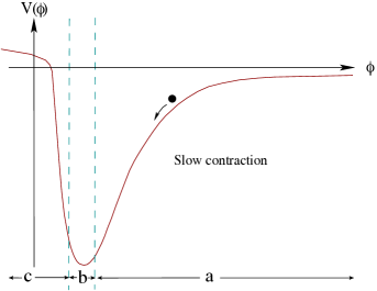
III.2.2 BKL instability
A bounce can be disrupted when an instability to the growth of anisotropy is present, see for instance Sec. V.2, so that the energy corresponding to anisotropy dominates. In 1970, Belinsky, Khalatnikov and Lifshitz (BKL) showed that any initial anisotropy grows unstable as the universe contracts towards a big crunch Belinsky et al. (1970). It can then be amplified sufficiently in a contracting phase to spoil a bounce if Belinsky et al. (1970); Lifshitz and Khalatnikov (1963); this BKL instability can be avoided by means of an ekpyrotic phase, for which . However, if spatial curvature is amplified and dominates, a mixmaster phenomenon takes place, in which space contracts and expands in different directions. The result is an inhomogeneous, anisotropic, singular crunch Misner (1969).
It has been argued that such a mixmaster behavior can also occur in
models with ultra-stiff matter, , Barrow and Yamamoto (2010):
assuming anisotropic pressures in such models, Barrow et al. argued
that the isotropic FLRW universe would cease being an attractor. Thus,
distortions and anisotropies are expected to be strongly amplified
during contraction in cyclic or ekpyrotic cosmologies. However, prior
analytic Erickson et al. (2004) and numerical studies
Garfinkle et al. (2008) of an ekpyrotic contraction showed that while
anisotropies and inhomogeneities indeed grow in some regions, leading
to an effective equation of state parameter , other regions
remain smooth and isotropic. The proper volume ratio of the latter to
the former grows exponentially along time slices of constant mean
curvature. In this sense, the ekpyrotic smoothing mechanism is indeed
effective in avoiding the mixmaster behavior in most, if not all,
regions.
As we show below, such an ekpyrotic phase discussed in Sec. III.2.1 could generate, just as in inflation, an almost scale-invariant curvature perturbation spectrum Battarra and Lehners (2014). Whether or not this can be made to agree with the observational data is a different topic, as one then needs to transfer these perturbations through the bouncing phase, see Sec. IV.6.
III.2.3 NEC violation
The success of a bounce depends on several factors. First and foremost, the Hubble parameter must change its sign from negative to positive at the bounce, commonly requiring the violation of the Null Energy Condition (NEC) in the framework of GR,
| (35) |
where is an arbitrary null vector (); for an ideal fluid with stress-energy tensor given by (5), Eq. (35) is equivalent to , which implies, since ( being timelike and lightlike),
| (36) |
Indeed, in the absence of curvature, the Einstein equations imply
| (37) |
which, along with (36), prohibits a nonsingular bounce: in order to have a Hubble rate always increasing from negative to positive values, the null energy condition must be violated for a finite amount of time , i.e. for around the bounce time. Hence, the violation of the NEC is crucial for models with vanishing (or negative) spatial curvature described by GR that weave together a contraction and an expansion phase.
The violation of the NEC usually leads to ghosts, indicating dangerous instabilities at the classical and/or quantum level and superluminality Dubovsky et al. (2006). See Rubakov (2014) for a recent review. Ghosts can be avoided in certain set-ups by employing, for example, a ghost condensate (higher derivatives) Arkani-Hamed et al. (2004); Creminelli et al. (2006), conformal galileons Nicolis et al. (2009) (conformally invariant scalar field theories with particular higher-derivative interactions) Creminelli et al. (2013a) or DBI conformal galileons (a 3-brane moving in an anti-de Sitter bulk, AdS5), used, for example, in the inflationary models of DBI Genesis Hinterbichler et al. (2013).
Desirable properties for a healthy bounce according to Hinterbichler et al. (2013); Elder et al. (2014) include,
-
1.
A stable Poincaré-invariant vacuum.
-
2.
The scattering amplitude about this vacuum obeys standard analyticity conditions.
-
3.
A time-dependent, homogeneous, isotropic solution which allows for a stable violation of the NEC.
-
4.
A subluminal propagation of perturbations around the NEC-violating background.
-
5.
A stable solution against radiative corrections.
Many proposed bouncing models have problems satisfying these conditions, as shown in table 3 taken from Elder et al. (2014) for a limited selection of models, highlighting the improvements of some iterations within the framework of galileon theories. Elder et al. (2014) provides an extended review of what is presented here. The models in this table are comprised of a ghost condensate Arkani-Hamed et al. (2004), Galileon genesis Nicolis et al. (2010, 2009); Creminelli et al. (2010); Creminelli et al. (2013a) based on conformal galileons, DBI genesis de Rham and Tolley (2010), and a recent proposal by Elder, Joyce and Khoury (EJK model) Elder et al. (2014).
A common stumbling block is superluminality, which only the most recent iterations of galileon models were able to avoid. It was further argued in Creminelli et al. (2013b); de Rham et al. (2013) that Galileon theories plagued with superluminality can be mapped into their dual analogues, which are free of superluminality; this idea has not yet been employed elsewhere.
As argued in Elder et al. (2014), any theory needs to admit a smooth interpolation between a Poincaré-invariant vacuum and the NEC-violating region. Such a smooth interpolation is impossible in a single-field dilation invariant theory Rubakov (2013) (see also Abramo and Pinto-Neto (2006) in the different but related context of phantom dark energy). By relaxing the assumption of dilation invariance, the EJK model in Elder et al. (2014) admits a solution that allows not only a healthy interpolation between a NEC-satisfying phase at early times and a NEC-violating phase at late ones, but is also subluminal.
Since many recent proposals of bouncing cosmologies employ ghost condensates and/or galileons, see table 2, we provide in the next section a brief introduction to the galileon theories outlined above, even though they are not bouncing models on their own. The cosmological super-bounce Koehn et al. (2014), based on the incorporation of a galileon into supergravity, avoids the problem of superluminality and is one of the more promising bouncing models to date.
III.3 Frameworks and partial answers
Implementing a bounce is not an easy task since the underlying theory must have many new properties. In order to be capable of having a bouncing solution, the theory must accommodate the violation of the NEC without initiating instabilities, which would spoil the very existence of the bounce. For instance, whatever the value of the spatial curvature, a bouncing phase initiated by a perfect fluid with energy momentum tensor (5), even including entropy modes, will always be absolutely unstable in the framework of GR Peter and Pinto-Neto (2002a).
Viewing General Relativity as a low energy effective theory, there are two basic options: to modify gravity or to consider matter content with special properties. A third alternative is to consider non-perturbative results in string theory. After a brief excursion on modified gravity models we introduce galileon theories, since this special class of exotic matter exhibits desirable properties for building bouncing cosmologies. For instructive purposes we follow with one concrete example, the matter bounce, which employs galileon fields. We conclude with two models based on T-duality in string theory, the S-brane bounce and a Hagedorn phase in string gas cosmology; the bounce in the latter set-ups is not describable within General Relativity or dilaton gravity, but is based on non-perturbative symmetries.
| Ghost condensate | Galilean Genesis | DBI Genesis | EJK Theory Elder et al. (2014) | |
|---|---|---|---|---|
|
|
✓ | ✓ | ✓ | ✓ |
| No ghosts | ✓ | ✓ | ✓ | ✓ |
| Sub-luminality | ✓ | ✓ | ✓ | ✓ |
| Poincaré vacuum | ✗ | ✗ | ✓ | ✓ |
| No ghosts | – | – | ✓ | ✓ |
| S-Matrix analyticity () | – | – | ✓ | ✓ |
| Sub-luminality | – | – | ✗ | ✓ |
| Interpolating solution | – | – | ✗ | ✓ |
| Radiative stability | ✓ | ✓ | ✓ | ✗ |
III.3.1 Modified gravity
There are many ways to modify gravity. Historically, the first models included a scalar mode in addition to the metric (a tensor) of General Relativity; since these scalar tensor theories are equivalent to ordinary GR with a modified matter content, we do not consider them separately. More complicated theories have been suggested, where terms are added to render the cosmological evolution explicitly singularity-free Brandenberger et al. (1993). Such models, which are appropriate to describe a bouncing phase, can be expressed as
| (38) |
where the are undetermined functions of curvature invariants, related to the Lagrange multipliers through the Euler-Lagrange equation . Demanding that for and for , with a constant, the theory reproduces GR for low curvatures and yields a de Sitter solution for high curvature. Bouncing solutions can be implemented in this framework Abramo et al. (2010); these solutions are stable and connect a contracting de Sitter phase to an expanding one.
Massive gravity can also lead to bouncing solutions. Defining gravity with respect to a de Sitter metric, bouncing solutions exist Langlois and Naruko (2013), if positive spatial curvature is present, even for a fluid satisfying the strong energy condition . However, these solutions are either doomed by a future singularity (curvature singularity or one that is unique to massive gravity) or tend to an asymptotic de Sitter regime.
Generically, modifications of gravity are expected to arise after quantization of gravity. Methods employing high energy physics have been proposed, most notably string theory, in which case one may often switch from the point of view of modified gravity to new components of the energy momentum tensor, as discussed in Sec. III.3.5. Similar attempts have been made in Loop Quantum Gravity (see Sec. II.1.1).
As we discussed in Sec. II.2, a complementary approach one may contemplate consists in an effective low-energy modification, as in the Wheeler-De Witt approach, whereby quantization is attempted in a super-space consisting of the set of all possible 3-metrics . Such an approach is usually unfeasible unless an additional mini-superspace approximation is performed, in which the infinite number of degrees of freedom is reduced to a few, for instance by considering only homogeneous and isotropic metrics. In Acacio de Barros et al. (1998), it was shown that in the presence of a simple perfect fluid, the singularity can always be avoided, independent of the fluid’s equation of state and the spatial curvature. Moreover, perturbations in such models can be treated self-consistently. In Peter et al. (2006); Pinho and Pinto-Neto (2007), a model dominated by a dust-like perfect fluid was shown to produce a scale-invariant spectrum of perturbations Peter and Pinto-Neto (2008), otherwise commonly obtained in the so-called matter bounce (see Sec. III.3.3). As this review aims at concentrating on classical GR or modifications thereof, we shall now move on to the second option to implement a bounce, namely that of changing the constituent behavior acting as a source in the Einstein equations.
III.3.2 Modified matter content
Ghost fields
To violate the NEC by brute force at the phenomenological level, one may include a ghost field with the Lagrangian
| (39) |
where has a canonical kinetic term with the wrong sign. In the absence of a potential (), the energy density and pressure are equal (), so that and the NEC is violated. Such an inclusion produces large amounts of adiabatic perturbations Peter and Pinto-Neto (2002a), because intrinsic entropy modes are absent. To counter this instability and render the total energy density positive, one may couple the negative energy fluid to an ordinary perfect fluid with positive energy, such as radiation. The resulting entropy modes, which were previously absent, render the model phenomenologically viable: using a free scalar field to mimic a stiff fluid (i.e. one with an equation of state parameter ), such a model was shown to be stable. The conditions to produce a scale-invariant spectrum of perturbations were calculated in Peter and Pinto-Neto (2002b). This model, however intrinsically problematic because relying on an unstable negative energy field, may be seen as a precursor of a ghost condensate: the temporary effective violation of the NEC merely permits the bounce to occur, but the negative energy component is otherwise subdominant for most of the universe history. No implementation was suggested in practice (see also Chimento and Forte (2006) for a bounce introduced by K-essence, where the conditions for a regular bounce, as well as anisotropies, were discussed): A more general phase space analysis of models with generalized kinetic terms can be found in De-Santiago et al. (2013), where conditions under which a bounce is possible in the NEC violating regime are derived.
The same idea was applied to the special situation in which, instead of radiation, the positive energy fluid is a scalar field whose dynamics is driven by an exponential potential Allen and Wands (2004), providing a model for the matter bounce. Contrary to many other bouncing models, the amplitude of tensor modes can be large, of order Allen and Wands (2004); Cai et al. (2009b), with a scale-invariant spectrum, in excess of current measurements, see Sec. IV.3.
Xue et al. studied in Xue et al. (2013) the evolution of fluctuations (in the same framework) non-perturbatively by means of simulations. They found that some regions of space could undergo a regular bouncing epoch, provided initial conditions were sufficiently close to being homogeneous and isotropic, while other regions would collapse, see Sec. IV.1 for details. Similar to a multiverse version of inflation, in which causally disconnected pieces of the Universe behave in different ways, our observable part is but a small patch of the full cycling multiverse.
Evidently, while simple ghost fields are unrealistic, the resulting
simplicity of bouncing models enables one to address otherwise
inaccessible questions.
Ghost-condensate
As summarized in Elder et al. (2014), the violation of the NEC in theories that involve one derivative per field, , implies the existence of either ghosts, gradient instabilities or superluminal propagation of perturbations Dubovsky et al. (2006); Buniy et al. (2006). In the previous paragraph, we discussed a few models which assumed such ghost fields for a finite duration. This can be implemented explicitly in the ghost-condensate technique according to which a field manages to violate the NEC only for some time, being dynamically driven first into this regime, and subsequently out of it.
A ghost condensate Arkani-Hamed et al. (2004) can arise from a higher-derivative theory containing the Lagrangian density
| (40) |
where the pressure function is an arbitrary differentiable function of the standard kinetic energy term
| (41) |
and which, in the cosmological context in which the scalar field depends only on time, reads ; the canonical kinetic term of (9) is obtained in the limit where . Using the flat FLRW metric (2) with , the scalar equation of motion becomes (we follow Koehn et al. (2013b) in this section)
| (42) |
If is a constant, (42) is trivially satisfied. However, if is a constant and at , the equation of motion allows for the ghost-condensate solution
| (43) |
The energy density is given by
| (44) |
where the pressure is identified with the Lagrangian function . Since, by definition, , a violation of the NEC can only result provided there exists a region for which . Therefore, the shape of the function should have a local minimum, denoted by in Fig. 11 which shows schematically the typical shape of enabling a temporary NEC violating phase. The theory is well-behaved near the ghost condensate point, if seen as an effective description of only the bounce – the model is self-consistent and does not contain a ghost. However, if seen as a fundamental theory, the model is problematic since it does not exhibit a Lorentz-invariant vacuum Elder et al. (2014): to avoid ghosts, has to hold. On the other hand, we need for a Lorentz-invariant vacuum, which cannot be reached from the minimum of at without inducing pathologies.
In the validity range of the ghost condensate regime, the Einstein’s equations (6) imply
| (45) |
so that a nonsingular bounce is possible in this regime. This mechanism was employed in Creminelli et al. (2006) and in the new Ekpyrotic scenario Buchbinder et al. (2007a); Creminelli and Senatore (2007); Buchbinder et al. (2007b), which, however, suffers from several instabilities Xue and Steinhardt (2010); see Sec. V. It was also implemented as the bounce mechanism for the matter bounce in Lin et al. (2011).

In the next subsections we investigate galileon theories which can
improve upon the ghost condensate.
Galileon genesis
An alternative to violate the NEC without introducing gradient instabilities is given by conformal galileons Buniy et al. (2006); Nicolis et al. (2010) (see also Kinetic Gravity Braiding Deffayet et al. (2010a) used in the G-bounce Easson et al. (2011)). The simplest conformally-invariant galileon Lagrangian in Creminelli et al. (2010) takes the form (we follow again Elder et al. (2014)),
| (46) |
where is the galileon field and and are constants. This theory has a time-dependent solution, with for . To remain within the confines of EFT we need so that . Since161616We corrected a typo in Elder et al. (2014). Nicolis et al. (2010); Creminelli et al. (2013a); Creminelli et al. (2010)
| (47) |
the NEC is violated for this solution. Furthermore, perturbations are stable and propagate luminally, but small deformations of the solution, which break homogeneity/isotropy Easson et al. (2013), lead to superluminality.
To avoid superluminality, Creminelli et al. (2013a) reduced the symmetry by considering a deformation of the original Lagrangian (46) to
| (48) |
where is a dimensionless parameter of order unity. The case breaks conformal invariance, while preserving dilation invariance. The solution for the galileon is unchanged, while is simply rescaled. The time-dependent solution violates the NEC if
| (49) |
is negative, requiring
| (50) |
Expanding the Lagrangian around this solution to second order, one can read off the speed at which perturbations propagate, namely
| (51) |
In order to avoid instabilities we need and in order to avoid superluminality we need . Thus the NEC can be violated while retaining stability and subluminality for
| (52) |
Similar to the ghost-condensate model, no Lorentz-invariant vacuum is present, even if the set-up were extended to include higher-order conformal galileons Creminelli et al. (2013a). However, perturbations are stable on all scales, opposite to ghost-condensate models, which are unstable on large scales during the NEC-violating phase.
Lagrangians of the above type are used in the galileon genesis
scenario
Nicolis et al. (2010, 2009); Creminelli et al. (2010); Creminelli
et al. (2013a),
among other proposals Deffayet
et al. (2010a); Kobayashi et al. (2010).
DBI genesis via conformal galileons
Even though the aforementioned models lack a Lorentz-invariant vacuum, either one of them may describe our Universe as an effective theory during the bounce; nevertheless, none of them can be seen as a fundamental theory. To improve upon this shortcoming, even more complicated galileon theories have been considered, while still avoiding superluminality. An example is to consider Dirac-Born-Infeld (DBI) conformal galileons Hinterbichler et al. (2013), as summarized in Elder et al. (2014), which we follow below. These theories describe the motion of a 3-brane by means of an effective scalar field in an geometry. The resulting 4D Lagrangian for is given by Hinterbichler et al. (2013)
| (53) |
where
| (54) | |||||
| (55) | |||||
| (56) | |||||
| (58) | |||||
with free coefficients , and
| (59) |
is the Lorentz factor for the brane motion; denotes the matrix of second order derivatives , , and , with indices raised by the Minkowski metric Nicolis et al. (2009). The are Lovelock invariants and guarantee second order differential equations de Rham and Tolley (2010).
Suitable choices of the free coefficients, ’s, allow for a
solution , leading to the stable violation of
the NEC Hinterbichler et al. (2013). A nice feature of this model is
that the speed of sound of fluctuations is subluminal while preserving
conformal invariance; further, the solution is stable against
radiative corrections and a stable Poincaré-invariant vacuum is
present. However, weak-field deformations of the vacuum may again lead
to superluminality and it is not clear if this is a mere pathology
Creminelli
et al. (2013b); de Rham et al. (2013) and how it should be cured.
Nevertheless, this is the first model in the literature that allows
the coexistence of a NEC-violating solution and a stable
Poincaré-invariant vacuum, although no interpolating solution
between them is given in Hinterbichler et al. (2013).
Elder, Joyce, Khoury (EJK) model
A smooth transition from a Poincaré-invariant vacuum to a NEC-violating phase is necessary, if such a model is to be used to generate a bounce. Rubakov showed in Rubakov (2013) that such an interpolation is impossible in single-scalar field theories that obey dilation-invariance. Violating the latter, a time-dependent, smooth interpolation between such solutions is presented in Elder et al. (2014) (we refer to this work as the EJK model). There, the galileon Lagrangian (46) is generalized to
| (60) |
where, and break scale invariance and are chosen to interpolate between a NEC satisfying solution at early times and a violating one at late times. In Elder et al. (2014), these functions are taken to be
| (61) | |||||
| (62) |
where and are constants. For suitable choices of these parameters, it was shown in Elder et al. (2014) that this model contains most of the necessary ingredients for a stable bounce: a Poincaré-invariant vacuum, stable, subluminal perturbations and an interpolation to a NEC-violating phase. See table 3 for a reproduction of the results presented in Elder et al. (2014).
To summarize, particular galileon theories appear to be promising candidates to construct nonsingular bouncing models that avoid pathological problems associated with the violation of the NEC such as ghosts, instabilities and/or superluminality.
III.3.3 Example: a nonsingular matter bounce
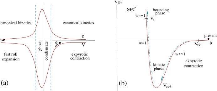
Nonsingular bouncing models are attractive since four dimensional General Relativity remains applicable throughout. The price one pays is that a component to the energy content of the universe must violate the NEC, often leading to dangerous instabilities, see Sec. III.2.3 and Sec. V. This was emphasized for instance in Xue and Steinhardt (2011) in which the action, besides gravity, is that a of a scalar field with Lagrangian,
| (63) |
where the function is depicted in Fig. 11 and the potential is illustrated on the right hand side of Fig. 12. In such an approach, the ekpyrotic phase must last a sufficiently long time in order to drive the shear contribution in (21) to vanishingly small values. At this stage, the universe enters a rapid phase of kinetic domination (labeled “kinetic phase” in Fig. 11) driving the field to the minimum of its potential and hence, to the ghost-condensate point. At this stage, the Hubble rate is large and negative, so that the ensuing phase must also last a long time in order to lower . Once the field has passed the ghost-condensate value, the NEC is violated, allowing for a bounce to eventually take place; this long period of NEC violating contraction tends to increase the shear exponentially, thereby ruining the benefit of the ekpyrotic phase.
A proposal that appears to avoid this instability is given in Cai et al. (2012a). In this model, the curvature fluctuations are expected to be scale invariant due to the presence of a matter phase and the bounce is nonsingular, bypassing the initial big bang singularity171717 The nomenclature to call this bounce a “matter bounce” is unfortunate as the model requires no prior matter dominated contraction phase; it is, nevertheless, used as such in the literature.. The universe undergoes a contraction, stops and reverses to expansion at a finite value of the scale factor while General Relativity remains valid. The NEC is violated via a ghost condensate and a galileon field. Adopting the form of the Kinetic Gravity Brading (KBG) model of Easson et al. (2011), the Lagrangian is
| (64) |
where and are functions of a dimensionless scalar field
| (65) |
The value of is chosen so that the kinetic term is bounded from below at high energy scales and the dimensionless function is chosen so that a phase of ghost condensation occurs briefly when approaches , see Fig. 12(a); is a galileon type operator,
| (66) |
with a positive-definite number and
| (67) |
This term is introduced to stabilize the gradient term of perturbations. The potential is shown in Fig. 12 together with the function . This function has a maximum which is only slightly larger than unity. The dynamics differs considerably from that of the previous model: right after the ekpyrotic contraction that suppresses the shear to negligible values, the NEC is only violated briefly, leading to a rapid bounce immediately followed by a fast-roll expanding phase. The shear growth is present, but has no time to develop efficiently, leading to logarithmic growth only. When expansion takes over, the shear decreases again: it is easy to set up initial conditions such that this shear never dominates the overall dynamics181818 Note that in this model, a large, flat, empty universe is assumed. These initial conditions may be seen as unnatural and hence highly fine-tuned.. The schematic of such a bounce is illustrated in Fig. 13.
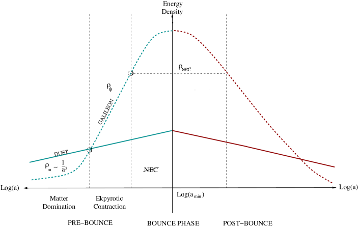
Specifically, using the matter action (64) leads to the modified Einstein equations
| (68) | |||||
where and denote derivatives of with respect to and respectively.
To achieve a nonsingular homogeneous bouncing solution with an ekpyrotic phase of contraction, the authors of Cai et al. (2012a) choose the potential,
| (69) |
where is a positive constant with mass dimension and , are free parameters (see Fig. 12a for a schematic). The choice of is crucial for the success of a nonsingular bounce, since should dominate the kinetic term for to violate the NEC. The function
| (70) |
with free parameters , and , was chosen in Cai et al. (2012a).
To summarize, the model entails the choice of two free functions and and 2 constants, which in Cai et al. (2012a) reduces to the specification of parameters, namely ; a set of numerical values was then chosen, among many others, merely to provide a proof of concept to illustrate a bounce that avoids the BKL instability: the calculation was done in the Bianchi I case in which a flat, homogeneous but anisotropic Universe contracts under the domination of a dust-like fluid. As mentioned above, the resulting curvature perturbations are scale invariant as shown in Wands (1999). The instabilities discussed in Sec. V are not present in this context because the bounce is rapid and immediately followed by a rapid expansion that counterbalances any prior increase of the shear, which is produced marginally (logarithmically) during the bounce. The duration of the bounce, which is short in comparison to the Hubble time just before it, is however long enough to ignore quantum gravity corrections, which would spoil the predictability of the model.
III.3.4 The cosmological super-bounce
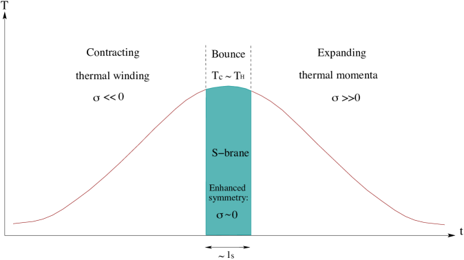
Based on prior work in Cai et al. (2012a), Lehners et al. constructed a super bounce in Koehn et al. (2014) based on a galileon Lagrangian given by
| (71) |
where
| (72) |
is the usual ekpyrotic potential, as depicted in Fig. 12(a), and
| (73) | |||||
| (74) | |||||
| (75) |
while , and are constants. These functions are chosen such that the effective ghost condensate and the galileon term violate the NEC briefly, leading to a bounce. The functions and are non-zero as passes through zero to prevent a singularity. Opposite to Cai et al. (2012a), where and , the higher derivative terms turn off for large values of , particularly during the ekpyrotic phase, to simplify an implementation into supergravity. The functional form of , and entails considerable freedom of choice.
As mentioned in Sec. II.6, the above Lagrangian can be implemented in supergravity after a computational tour de force, see Koehn et al. (2014) for details. The resulting bounce is devoid of the many pitfalls reviewed in Sec. V, and thus, at the time of writing, one of the most successful nonsingular bouncing models, see Table 2.
Observables, such as the scalar spectral index and non-Gaussianities, are consistent with the known results in ekpyrotic scenarios, see Sec. IV, since curvature perturbations stay frozen on super Hubble scales during the bounce, as shown in Battarra et al. (2014): here, the computation was performed in the harmonic gauge with a detailed discussion of the validity of linear perturbation theory, see Sec. IV.1.
III.3.5 Models based on T-duality in string theory
S-brane models
String theory is a UV complete theory of quantum gravity and as such, it provides a consistent framework for model building. Hence, a cosmological model free of singularities should be feasible via the incorporation of fundamental duality symmetries and stringy degrees of freedom in a time-dependent setting, see Florakis et al. (2011); Kounnas et al. (2012a, b); Kounnas and Toumbas (2013) and Kiritsis and Kounnas (1994); Cornalba and Costa (2002, 2004) for early work.
An example in type II superstring theory, , compactified to four dimensions entails a weakly coupled string gas as a thermal component to enable a bounce Florakis et al. (2011); Kounnas et al. (2012a, b). Such a nonsingular cosmological scenario in dilaton gravity is usually hindered by the appearance of Hagedorn instabilities, which occur at a critical temperature close to the string scale, GeV (the Hagedorn Temperature), and signal non-trivial phase transitions Atick and Witten (1988); Antoniadis and Kounnas (1991); Barbon and Rabinovici (2002, 2004). The Hagedorn singularity as well as the big bang singularity can be resolved Kounnas et al. (2012a); the nonsingular191919 The S-brane’s delta function source is a delta function in temperature and thus, in time. Therefore, it does not constitute a singularity with respect to curvature invariants, which we take as the definition of a singular bounce. In essence, this delta function source is conceptually closer to the presence of D-branes and indeed cosmological perturbations can be matched across the S-brane unambiguously. The string theoretical description of the S-brane bounce goes beyond the scope of this review and we refer the interested reader to the original literature Florakis et al. (2011); Kounnas et al. (2012a, b). cosmological evolution is governed by a phase transition, described in terms of a spacelike brane (S-brane202020The S-brane may be viewed as a defect that interpolates between the two distinct geometrical phases of the underlying conformal field theory. At the level of the low energy effective description, the condensate of massless states that appears at forms a short-lived, space-filling object, whose lifetime is comparable to the temporal resolution of the EFT and is therefore modeled as a delta function. At the CFT level, an operator becomes marginal at which converts directly winding states into momentum ones with a coefficient determining the efficiency of this interaction proportional to .), between two dual thermal phases.
This setup realizes temperature duality (T-duality) of string theory Florakis et al. (2011); Kounnas et al. (2012a, b); Kounnas and Toumbas (2013). The crucial component in this scenario is a thermal string gas, see Brandenberger and Vafa (1989); Tseytlin and Vafa (1992) and Kalyana Rama (1997); Bassett et al. (2003); Easther et al. (2005); Battefeld and Watson (2006); Kaloper and Watson (2008); Brandenberger (2008); Greene et al. (2009) for reviews on string gas cosmology and early work: light thermal momentum modes and light thermal winding modes exchange roles via T-duality. Near the critical temperature, new light degrees of freedom appear due to an enhanced symmetry, giving rise to the S-brane which serves as a glue between the two dual thermal phases. The S-brane has localized (in time) negative pressure, but no energy density. It thus violates the NEC in a controlled manner; in the low energy description, the S-brane, which has a thickness set by the string scale, can be treated as a -function source in the Einstein equations. Since the violation of the NEC is extremely brief, the instabilities hampering a ghost-condensate bounce, see Sec. III.3.2, are absent.
The action of the physical system in the string frame, denoted by a tilde, reads
where is the dilaton, is the determinant of the string frame metric, is the corresponding Ricci scalar, the pressure of the thermal string gas, is the determinant of the induced metric at the location of the S-brane, is the brane tension and is the inverse of the temperature. For more details see Kounnas et al. (2012a, b); Kounnas and Toumbas (2013); Brandenberger et al. (2013). Since the thermal string gas has a constant equation of state, it can be modeled by a derivatively coupled scalar field via
| (77) |
where is the number of massless degrees of freedom and is Boltzmann’s radiation constant. Hence, the temperature is identified with
| (78) |
a relation which continues to hold at the perturbed level.
The dilaton and the scale factor in the Einstein frame reverse at the critical temperature , with the latter’s bounce corresponding to a smooth reversal of contraction to expansion so that the big bang curvature singularity is absent; at the phase transition the dilaton attains its maximal value, determined by the brane tension, the critical temperature , and the number of thermally excited massless degrees of freedom; as a consequence, the transition can take place entirely in the weakly coupled regime.
Each of the three phases, contraction, bounce and expansion, admits a local effective field theory description Kounnas et al. (2012a): the temperature in the contracting regime can be identified with the inverse period of the Euclidean time cycle, . The expanding phase corresponds to the dual of the contracting one with and temperature . Defining the thermal modulus , we have
-
1.
Contraction: light thermal windings regime, , ( and , i.e. large and negative).
-
2.
Bounce: enhanced symmetry regime – thermal states become massless, , ().
-
3.
Expansion: light thermal momenta regime, , ( and , i.e. large and positive).
Fig. 14 shows a schematic representation of these phases.
To study fluctuations, one needs to perturb the metric and the dilaton together with the thermal component. Modeling the latter via a derivatively coupled scalar field Mukhanov (2005); Dubovsky et al. (2006); Boubekeur et al. (2008), the transition of fluctuations between contracting and expanding phases is studied in Brandenberger et al. (2013). Applying the Israel junction conditions Israel (1966), Sec. IV.2.5, across the S-brane, the curvature fluctuation in the expanding phase can be computed from the perturbations generated via quantum fluctuations in the degrees of freedom during the contracting phase. Incorporating a matter dominated phase during contraction Wands (1999), a scale-invariant spectrum of curvature perturbations can be generated at late times. A tilt of the power-spectrum may result from changes to the speed of sound caused by the dilaton admixture to the matter fluid, but a computation of this effect has not been performed yet.
This implementation of a nonsingular bounce in string theory is a
promising proof of concept. However, the current proposal suffers from
several short-comings: for instance, since no ekpyrotic phase is
present, the BKL instability commonly arises Belinsky et al. (1970),
see Sec. III.2.2. It may be problematic to incorporate an ekpyrotic
field, see Sec. III.2.1, since its fast growing energy
density might dominate over the thermal component. It was argued in
Brandenberger et al. (2013) that the presence of kinetic energy in
the dilaton, which also redshifts as , would alleviate the
problem to some degree. However, it is crucial that the thermal
component dominates during the bounce, hence, fine-tuning appears
unavoidable. Lastly, since the temperature is usually very high,
GeV,
thermal relics, such as gravitinos, and potentially topological
defects from phase transitions, such as magnetic monopoles, may be
produced Battefeld and
Battefeld (2009a) (see Sec. III.1.4), but this is
model-dependent. In addition, large non-Gaussianities may be produced
Gao et al. (2014b, c).
A Hagedorn phase in string-gas cosmology

In a speculative, yet interesting proposal motivating the above S-brane bounce, Brandenberger, Vafa and Nayeri Nayeri et al. (2006); Brandenberger et al. (2006a) (see Brandenberger (2011a); Battefeld and Watson (2006) for reviews and Kaloper and Watson (2008); Kaloper et al. (2006) for criticisms) attempted to generate a scale-invariant spectrum of density fluctuations via temperature fluctuations during a quasi-static Hagedorn phase of a string gas comprised of closed heterotic strings212121The S-brane bounce has its roots in string-gas cosmology, but operates in Type II string theory, opposite to the models of this section in heterotic string theory. Note that the role of T-duality also differs, as it involves the Euclidian time cycle in the S-brane bounce, and the scale factor of a toroidal compactification in string-gas cosmology.. If the dilaton and all other moduli fields are assumed to be stabilized at these high temperatures, the resulting spectrum is indeed scale invariant. A tilt is introduced through the transition from the Hagedorn phase to a radiation dominated expanding FLRW universe. This model may be viewed as a bounce if a pre-Hagedorn phase is introduced via T-duality, see Fig. 15. A concrete realization (that is free of ghosts) invokes an infinite number of higher derivative interactions, see Biswas et al. (2007). Alternatively, this proposal can be seen as an emergent universe without a bounce.
This model also predicts an observably large gravitational wave spectrum, similar to inflationary slow roll models, but with a slight blue tilt Brandenberger et al. (2014); Brandenberger et al. (2007b, a); Nayeri (2006), opposite to the inflationary red one. Thus, this model may be compatible with a high level of gravitational waves such as claimed by BICEP2 Ade et al. (2014a, c), see Eq. (146) below.
The string gas proposal has several points that need be addressed:
-
•
the flatness problem is not solved, but requires fine-tuned initial conditions,
-
•
a quantitative understanding of the Hagedorn phase is incomplete, so that the transition from the Hagedorn phase to a radiation-dominated FLRW universe cannot yet be computed. Due to the high temperature, , the use of General Relativity or dilaton gravity may not necessarily be justified. A phenomenological proposal for a nonsingular, ghost free bounce induced by an infinite series of higher derivative corrections was given in Biswas et al. (2007). If the Hagedorn phase is directly connected to the expanding FLRW phase, one should expect the over-production of thermal relics and topological defects (if present in the spectrum of the theory) from phase transitions, because the temperature is so high, as pointed out by one of the authors of this review in Battefeld and Battefeld (2009a),
-
•
keeping the dilaton dynamical, as one might expect at these high energies, destroys the scale invariance of this spectrum Kaloper et al. (2006). While dilaton gravity is not expected to be applicable during the Hagedorn phase, it is uncertain if all similar scalar quantities can be frozen during this phase, see footnote 33 in Sec. VI.2 for the related challenges of moduli stabilization.
IV Cosmological Perturbations
In addition to providing a solution to problems of the big bang, a bounce should produce almost Gaussian (i.e. with a low level of non-Gaussianities) perturbations whose spectrum is nearly scale invariant and slightly red in order to agree with current observations as revealed by the PLANCK data Ade et al. (2014b, 2013b, 2013c). Further, if the BICEP2 interpretation is confirmed, gravitational waves at the level of ought to be present at these scales Ade et al. (2014a). See however, Flauger et al. (2014); Mortonson and Seljak (2014) for a study highlighting that the polarization observed by BICEP2 might be caused by dust instead of primordial gravitational waves.
Given that a bounce is feasible, the aforementioned conditions impose severe constraints on the overall scenario, particularly during the contracting phase. If only a single degree of freedom is present in the contracting phase, so that the perturbations are adiabatic, the equation of state parameter must be in order to generate a nearly scale-invariant power spectrum222222A duality between contracting and inflating universes exists at the level of the power spectrum, see Wands (1999). Finelli and Brandenberger (2002). Models with are called “matter bounces” because their equation of state mimics that of ordinary dust; it does not imply the presence of actual matter, since such an equation of state can also be achieved by a scalar field oscillating in a quadratic potential. Alternatively, a scale-invariant power spectrum can be generated by an entropic mechanism, similar to the curvaton scenario, see Sec. IV.5. However, anisotropies/shear often arise, as discussed in Notari and Riotto (2002); Xue and Steinhardt (2010, 2011), which can spoil the bounce232323The generating mechanism of a scale-invariant power spectrum is essentially decoupled from the physics of the actual bounce. and/or the spectrum, see Sec. V. Entropic mechanisms also generate non-Gaussianities via the conversion mechanism, which are in tension with current observational limits, see Sec. IV.5.
An equation of state parameter larger than unity during the contraction (ekpyrotic phase) can prevent the growth of anisotropy/shear. Models whereby the bounce is realized via galileons, in which the Lagrangian contains higher order derivatives, avoid the appearance of ghosts while the extra additional degrees of freedom violate the NEC. Promising models which address the anisotropy problem in Galileon cosmology and might generate a scale-invariant spectrum include Chimento and Forte (2006); Cai et al. (2012a, 2013a); Koehn et al. (2014), see Sec. II.6.
Models with an ekpyrotic phase do not generate measurable gravitational waves, whereas matter bounce models generically predict a tensor-to-scalar ratio in excess of observational limits, see Sec. IV.3.
In the subsequent sections we discuss cosmological perturbations (scalar and tensor) and non-Gaussianities in a few concrete models. We do not aim to provide a complete overview of all proposals, but deliberately focus on some promising ones to explain the crucial steps of the computations and highlight important results with broad applicability.
IV.1 The viability of perturbation theory in a contracting universe
Is a perturbative analysis possible in nonsingular models? For singular models, such as the original ekpyrotic scenario, cosmological scalar perturbations diverge as Lyth (2002b), casting doubt on the perturbative treatment. In such scenarios, it is understood that at some point the 4D effective theory breaks down, and one has to resort to the full description in string theory. One might hope that the singularity and thus the divergence of perturbations is absent. However, merely going to the higher dimensional setting, for example, in the ekpyrotic universe Enqvist et al. (2001), and properly incorporating metric perturbations does not necessarily alleviate this problem, as shown in Battefeld et al. (2004). A similar problem is present for vector perturbations in a contracting universe Battefeld and Brandenberger (2004).
For a nonsingular bounce, perturbations are not necessarily divergent, but still strongly growing in the contracting phase. The current lore in the literature is that linear perturbation theory fails in some gauges, such as the longitudinal Lyth (2002b); Martin et al. (2002) and comoving ones Kodama and Hamazaki (1996), while it remains valid in others, for example, in the uniform field gauge Allen and Wands (2004). As shown in Xue and Steinhardt (2010, 2011), the curvature perturbation and anisotropy grow rapidly during contraction, casting doubt on the viability of perturbation theory, see Sec. V.
One of the first occurrences where this problem surfaced was the pre-big bang scenario, see Gasperini and Veneziano (2003) for a review. In Gasperini et al. (2004) it was argued that one could go to a gauge where scalar perturbations are at most logarithmically growing, but it should be noted that the usual gauge invariant variables still obey a power-law growth.
The question regarding the validity of the perturbative linear regime during the bounce is particularly evident in the longitudinal gauge due to the Newtonian potential’s rapidly growing mode Creminelli et al. (2005) – the Newtonian potential corresponds to the metric perturbation function in Eq. (83) below and equals the Bardeen Potential in this gauge Bardeen (1980). However, this mode becomes a decaying one during the expansion phase, hinting that this growth may be a gauge artifact and/or that is not a good tracer to check the validity of perturbation theory (one may define non-divergent, gauge-invariant variables by multiplying with appropriate background functions). It is possible to find other gauges in which this growing contribution is absent Allen and Wands (2004). A generalization of these ideas to a large class of models was attempted in Vitenti and Pinto-Neto (2012), where a set of conditions for linearity is obtained that allows the perturbative series to be valid. The spectrum of modes considered in Vitenti and Pinto-Neto (2012) became frozen during a matter dominated contracting phase, but the actual bounce was kept general. The conditions in Vitenti and Pinto-Neto (2012) arise by demanding that all terms in the perturbed Einstein equations remain small. One then obtains a set of conditions by requiring the smallness of the perturbed volume expansion rate as well as that of the second spatial derivative (the covariant Laplacian with respect to the spatial metric) acting on the two Newtonian potentials and in Eq. (83), as well as the shear, which is set by the off-diagonal metric perturbations. Of all the gauges considered in Vitenti and Pinto-Neto (2012), the synchronous gauge ensures that perturbations near the bounce stay finite and small at all times Vitenti and Pinto-Neto (2012).
This advantage of the synchronous gauge, as well as the presence of a dynamic attractor in the ekpyrotic scenario, was first pointed out in Creminelli et al. (2005). In the presence of the aforementioned attractor, the cosmological solution becomes locally homogeneous, isotropic and flat. Thus, as long as the bounce is not sensitive to exponentially small corrections, the bounce appears identical to every observer. As a consequence, unambiguous predictions can be made with respect to the spectrum of fluctuations. Based on this method, Creminelli et al. Creminelli et al. (2005) showed that the original single field ekpyrotic model does not possess a scale-invariant spectrum. It is further shown why the Bardeen potential generically diverges, see Sec. IV.2.3.
Linearity conditions can also be defined covariantly, as in Kumar (2012) for a radiation and dust-like single-fluid FLRW background. It has been claimed in Kumar (2012) that these conditions are violated as the scale factor shrinks and the bounce is approached. However, as shown in Pinto-Neto and Vitenti (2014), the conditions of Kumar (2012) reduce to the ones in Vitenti and Pinto-Neto (2012) and a violation of linear perturbations is not necessarily present.
Going beyond linear perturbation theory, a recent, interesting and encouraging study of adiabatic perturbations generated was performed in Xue et al. (2013). A simple model of the bounce was used to follow perturbations through a nonsingular matter-like contraction akin to Peter and Pinto-Neto (2002b); Allen and Wands (2004); Cai et al. (2008), see Sec. III.3.2, the actual bounce and into an expansion phase. The main goal of this study was to find a well-behaved gauge in which a non-perturbative numerical analysis can be performed. A pressing problem preventing the use of constant mean curvature slices, as commonly used in standard perturbative analysis, is that these slices stop being space-like during the transitions to the bouncing phase in the presence of inhomogeneities. A possible way out is provided by the use of the harmonic gauge, where coordinates satisfy the condition
| (79) |
which entails
| (80) |
In this gauge, coordinate singularities are absent during the bouncing phase when and are non-monotonic. Further, the equations of motion for metric components are wave-like and thus easy to solve. In Xue et al. (2013) results in the harmonic gauge were also translated to the commonly used non-linear generalization of the curvature perturbation in the covariant formalism, . At the time of writing, the harmonic gauge appears to be the gauge of choice to compute unambiguously the evolution of perturbations in a bouncing universe.
The non-perturbative, numerical solutions in Xue et al. (2013) show that the universe does bounce in regions where the universe is homogeneous and isotropic enough. More precisely, the universe undergoes a nonsingular bounce in regions where the ratio between energy density in the anisotropy [see Eq. (21)] and that of the field satisfies,
| (81) |
On the other hand, in regions where
| (82) |
the universe crunches: since energy in the ghost field, , drives the nonsingular bounce, and because it can never catch up with , the universe in this particular region collapses into a singularity.
If a nonsingular bounce takes place close to the critical ratio above, adiabatic modes are generically strongly coupled during the bounce, which affects the power spectrum and may generate large non-Gaussianities. However, if the perturbations are of the same order as the observed primordial ones, nonlinearities are unimportant, the bounce is unscathed, and the strong coupling problem for super-Hubble modes does not arise. Thus, in this case, the nonsingular bounce is not expected to lead to large non-Gaussianities Xue et al. (2013).
For more details on the use of the harmonic gauge see Battarra et al. (2014), which makes contact to other commonly used gauges and provides another application to the superbounce, see Sec. III.3.4: the validity of linear perturbation theory was tested and it was confirmed that the equations of motion for certain variables, such as the curvature perturbation in (84), contain singularities. However, in the harmonic gauge, the relevant equations are nonsingular and linear perturbation theory remains valid in this particular bounce model. Furthermore, it was found that long wavelength perturbations are unaffected by the bounce; hence, the pre-bounce power spectrum passes through the bounce unaltered.
In the following, we focus on the generation mechanism of a scale-invariant spectrum in the pre-bounce phase, employing the curvature perturbation . It should be understood that the harmonic gauge should be used to follow the perturbations through the bounce, as mentioned above, to check whether or not a spectrum survives in a particular bouncing model of the universe.
IV.2 Generating a nearly scale-invariant power spectrum in a contracting universe
Measurements of the cosmic microwave background radiation Ade et al. (2014b, 2013b, 2013c) reveal adiabatic, highly Gaussian temperature fluctuations with a nearly scale-invariant power spectrum. These fluctuations trace back to curvature fluctuations that must have been generated during a preceding inflationary or, as in our case, a contracting phase of the early universe Lehners (2011b). These fluctuations need to show correlations on super-Hubble scales at the time of decoupling, which can be achieved either during a rapid accelerated expansion or a slow contraction, see Wands (1999); Khoury et al. (2002b) for a duality at the level of the power spectrum between these two options. For example, during an ekpyrotic phase, quantum fluctuations cross the Hubble scales and are converted into classical, local density perturbations. The scaling solution (31) shows that the scale factor is almost constant, meaning that a mode’s wavelength stays also constant. The Hubble length, (assuming the bounce to take place at ), see Fig. 5, shrinks as , so that any mode eventually becomes super-Hubble close to the bounce.
We first provide a brief overview of cosmological perturbation theory Peter (2009); Mukhanov et al. (1992), following the review Bassett et al. (2006) in order to set our notation and then proceed by providing the computation of the power spectrum in a two-field ekpyrotic contracting universe as a concrete example of a bouncing universe. This computation highlights the failure of single field models, since they carry a deep blue spectral index, and explains the current preference of two-field models, whereby scale-invariant perturbations in an entropic field are subsequently converted to the adiabatic mode. We also introduce the formalism for our discussion of non-Gaussianities in Sec. IV.5. In addition, we show how a scale-invariant spectrum can arise in the adiabatic mode in a matter-dominated contracting universe. We briefly explain the Deruelle-Mukhanov matching conditions, which are invoked whenever distinct phases are attached to each other.
IV.2.1 Basics of cosmological perturbation theory
Our goal is the computation of the gauge invariant, comoving curvature fluctuation , which is commonly used to impose observational bounds. Consider the perturbed FLRW metric Mukhanov et al. (1992); Peter and Uzan (2009), including only scalar degrees of freedom,
| (83) | |||||
in conformal time. The four variables in the metric entail two degrees of freedom and two gauge modes. A popular choice is the Newtonian gauge where so that the gauge-invariant Bardeen potentials read and . The curvature perturbation on hypersurfaces orthogonal to comoving worldlines is defined as
| (84) |
where is the scalar field perturbation. This gauge-invariant variable coincides with on large scales, see Eq. (94) below. In Fourier space, one may define the so-called Mukhanov-Sasaki variable
| (85) |
with
| (86) |
and the wavenumber (see Sec. V.4 for the inclusion of a general speed of sound ). In the following, we provide expressions in the presence of many fields, which we denote with a latin subscript ; to avoid clutter, we often skip the Fourier index on variables. The curvature fluctuation is easily expanded by means of the formalism Starobinsky (1985); Sasaki and Stewart (1996); Sasaki and Tanaka (1998); Vernizzi and Wands (2006); Rigopoulos et al. (2006); Lyth and Rodriguez (2005) as,
| (87) | |||||
where , is the number of e-folds
| (88) |
using an initially flat hypersurface as well as a final uniform density hypersurface, , , etc. and .
It is useful to introduce the gauge-invariant Mukhanov-Sasaki variables
| (89) |
that satisfy the equations of motion in Fourier space Gordon et al. (2001),
| (90) |
Sometimes, rescaled Mukhanov-Sasaki variables are defined in the gauge as . Note that in models with only one scalar field and , the two rescaled Mukhanov-Sasaki variables are proportional to each other . These variables are defined such that the friction term in their respective equations of motion vanishes,
| (91) |
where a prime denotes a derivative with respect to conformal time.
Useful relationships between these variables are
| (92) |
and
| (93) | |||||
| (94) |
We freely switch between and in what follows, since we are only interested in the limit of large scales .
The power spectrum of curvature fluctuations is defined as the Fourier transform of the 2-point function,
| (95) |
One often defines a rescaled dimensionless power spectrum by
| (96) |
whose amplitude satisfies the COBE normalization Bunn et al. (1996) and we introduced the notation . Using the formalism Dvali et al. (2004), one may also compute the power spectrum via
| (97) |
where
| (98) |
The scalar spectral index is defined through
| (99) |
which has to equal the PLANCK measurement Ade et al. (2013c). Thus, a blue power spectrum (), such as that obtained in the simplest matter bounce, is ruled out.
Similarly, a tensor power spectrum can be defined, see Sec. IV.3, whose amplitude is usually constrained via the tensor to scalar ratio
| (100) |
which has to satisfy , according to PLANCK Ade et al. (2013c) and if the BICEP2 interpretation of the data is correct Ade et al. (2014a). See however, Flauger et al. (2014); Mortonson and Seljak (2014)
IV.2.2 Two-field ekpyrosis
As we shall see, it is impossible to generate a scale-invariant spectrum in the adiabatic mode during an ekpyrotic phase; this led to the investigation of two-field models Notari and Riotto (2002). Such scenarios are often natural in concrete settings in string theory and supergravity, see Koehn et al. (2014) for a recent example. The presence of at least two scalar fields gives rise to isocurvature (entropy) perturbations, which, in turn, can source curvature perturbations. Hence, if the isocurvature perturbations acquire a nearly scale-invariant spectrum, the curvature perturbations may inherit this spectrum via curvaton-like mechanisms, see Sec. IV.5 Notari and Riotto (2002); Lehners et al. (2007a).
In what follows, we review the origin of scale-invariant perturbations in an isocurvature mode during an ekpyrotic contracting phase. As a concrete example, consider two scalar fields , with canonical kinetic terms and an uncoupled, exponential potential
| (101) |
where and . The equations of motion are
| (102) |
and the Friedmann equations read,
| (103) | |||||
| (104) |
Eqs. (102–104) with potential (101) possess two attractor solutions, each corresponding to a single field ekpyrotic solution, whereby either or dominate. In addition to these two attractor solutions, there is a third alternative where the ratio of the kinetic energy to potential energy is constant; the adiabatic field along this trajectory is not an attractor.
Following the review Bassett et al. (2006), let us define,
| (105) |
and an isocurvature field perpendicular to it
| (106) |
The potential becomes
| (107) |
where and
| (108) |
which has a maximum at
| (109) |
The unstable solution corresponds to , while rolls down the exponential potential in (101). The resulting equation of state parameter satisfies . For this solution, is identical to the adiabatic field along the trajectory,
| (110) | |||||
| (111) |
whereas is the perpendicular isocurvature field.
The tachyonic instability in gives rise to a scale-invariant spectrum of perturbations in in a contracting universe242424Setting initial conditions to this solution may appear fine-tuned, but can be natural in the framework of the Phœnix universe, see Sec. III.1.5. We make the assumption that stays close to throughout so that and const. The Friedmann equations leads to a power law contraction with . From here onwards, we follow Battefeld (2008) (see also Tolley and Wesley (2007)) and switch back to conformal time so that
| (112) |
with defined below through Eq. (118).
The Mukhanov-Sasaki variable for multiple fields is defined in (89) and its equation of motion is given by (90). In the gauge, and . In terms of these variables, the comoving curvature perturbation is .
In the absence of a curved trajectory in field space, there is no conversion of isocurvature modes into adiabatic ones and the equations decouple: using and in Eq. (90), we obtain
| (113) | |||||
Working in conformal time and making use of and , the equations above reduce to
| (115) |
with and
| (116) | |||||
| (117) |
where we introduced
| (118) |
with the fast roll parameter defined in (27). Imposing the Bunch-Davies vacuum initial conditions well inside the Hubble radius so that can be neglected, we have
| (119) |
where satisfies . Keeping the term in the equation of motion we obtain
| (120) |
where are Hankel functions of the first and second kind respectively, with index
| (121) |
Expanding the Hankel functions for large arguments we can match from (119) and (120) to determine as
| (122) |
After Hubble crossing we can use the small argument limit of the Hankel functions to arrive at
| (123) |
where
| (124) |
The power spectrum in (98) becomes
| (125) |
so that we can read off the scalar spectral indices
| (126) |
Further expanding from (121) and (117) in terms of the fast roll parameter we obtain the spectral indices
| (127) | |||||
| (128) |
The adiabatic mode carries a deep blue spectrum as in single field ekpyrosis252525Since these modes are not amplified and thus their wavefunction is not squeezed, it has been argued that they cannot be described classically, as pointed out in Tseng (2013). As a result, the application of matching conditions, as delineated in Sec. IV.2.5, to the ekpyrotic scenario, would be flawed. In the entropic mechanism, perturbations become classical and the conversion process causes super-Hubble perturbations to fully decohere Battarra and Lehners (2014); the lack of amplification, and thus squeezing, of gravitational waves in ekpyrotic scenarios casts doubts on treating the latter classically, as done in Sec. IV.3 and Boyle et al. (2004). A study for gravitational waves similar to Battarra and Lehners (2014) has not yet been performed. Lyth and Wands (2002) and the isocurvature mode carries a small blue tilt, respectively. By choosing a slightly more complicated potential than the choice made in (101) one may also generate a slightly red spectrum for the isocurvature field Fertig et al. (2014), see also Lehners et al. (2007a); Buchbinder et al. (2007a). To reiterate, the isocurvature fluctuations still need to be converted into adiabatic ones in realistic models (Sec. IV.5), and to be passed through the bouncing phase to the expanding one.
IV.2.3 The growing mode in the Newtonian gauge
As explained in Sec. IV.1, the Bardeen potential commonly grows very large or even diverges as the bounce is approached, which is easy to see. For instance, using the same scaling solution as in the previous section, valid for the ekpyrotic scenario, (31), the equation of motion for becomes Khoury et al. (2002b)
| (129) |
The properly normalized solution is
| (130) |
where we used similar steps as in the previous section; hence, at late times
| (131) |
Evidently, the first term diverges as the bounce is approached, indicating that the Newtonian gauge should not be used close to the bounce. As we saw in Sec. IV.1, one should use the harmonic gauge to unambiguously follow perturbations through the bounce. Nevertheless, familiar gauges, such as the Newtonian one, can be used in the pre-bounce phase.
IV.2.4 Adiabatic fluctuations in a matter bounce
Instead of relying on an entropic mechanism, one may also generate a scale-invariant spectrum directly in the adiabatic mode if the background evolution conforms to a matter dominated phase Finelli and Brandenberger (2002). Cosmological models in which the contraction phase is dominated by a dust-like fluid leading to such a spectrum were studied in Gasperini and Veneziano (1993, 1994); Wands (1999); Brandenberger and Finelli (2001); Martin et al. (2002); Lyth and Wands (2002); Lyth (2002b); Khoury et al. (2002b); Durrer and Vernizzi (2002); Hwang and Noh (2002); Cartier et al. (2003).
To understand the origin of the scale-invariant spectrum, consider Eq. (115) for a single degree of freedom. If the scale factor evolves according to
| (132) |
one arrives at
| (133) |
Since the scalar spectral index in (126) reads
| (134) |
we need in order to get a scale-invariant spectrum. This corresponds to , that is, a matter dominated contracting phase. Such a phase need not be dominated by actual dust, but could be mimicked by an oscillating scalar field in a quadratic potential. The latter can also accommodate a slightly red spectrum by altering the potential Wands (1999). This matter bounce was first proposed in Wands (1999); Finelli and Brandenberger (2002); Brandenberger (2011b). Thus, there are two ways of getting a scale-invariant spectrum in the contracting phase: the matter bounce and the entropic mechanism discussed in Sec. IV.5.
IV.2.5 Matching conditions
In this section we sketch the Deruelle-Mukhanov matching conditions for cosmological perturbations in an FLRW universe at a sharp transition Israel (1966); Hwang and Vishniac (1991); Deruelle and Mukhanov (1995). At the hypersurface of the transition, the induced metric is continuous and the extrinsic curvature jumps according to the surface tension. In an ever-expanding or contracting FLRW setting and a simple jump in the equation of state parameter, they entail the continuity of the Hubble parameter and the scale factor at the background level. Furthermore, these conditions provide matching conditions for perturbations of the metric, as well as the perturbed energy momentum tensor. For details we refer the interested reader to the textbooks Mukhanov (2005); Peter and Uzan (2009).
These matching conditions are often crucial in nonsingular as well as singular bouncing models. For example, matching perturbations across the singular bounce in the original ekpyrotic scenario Khoury et al. (2001a) was performed in Finelli and Brandenberger (2002) in the effective 4D description. However, since the singularity is not resolved, ambiguities remain, which led to an extensive discussion of the proper matching conditions for a singular set-up. For example, Finelli and Brandenberger (2002) argued, based on Israel (1966); Deruelle and Mukhanov (1995), that only the decaying mode in the contracting phase couples to the dominant one in the expanding phase. In general, mode mixing is present in bouncing scenarios so that both modes, the subdominant and dominant ones, of the contracting universe determine the dominant mode (the relevant one as far as present-day observations are concerned) in the expanding phase Khoury et al. (2002b)262626Following Martin and Peter (2003), we call mode mixing the mixture of both dominant and sub-dominant (growing and decaying in the inflation literature) modes at fixed scale in order to avoid confusion with higher order mixing terms involving different scales..
In nonsingular set-ups, matching conditions are generally unnecessary because the evolution of perturbations can be followed, at least numerically, throughout the nonsingular bounce. However, to gain an analytic understanding of the resulting power spectrum and its sensitivity to model parameters, matching conditions are often invoked to stitch together distinct analytic approximations covering the contracting phase, the bounce and the expanding phase. The application of the matching conditions in Deruelle and Mukhanov (1995) requires the specification of a scalar quantity that determines the position of the transitional hypersurface. Once this quantity is specified, no ambiguities remain. Applications include Refs. Brandenberger and Finelli (2001); Bozza et al. (2003); Battefeld et al. (2004); Battefeld and Geshnizjani (2006); Geshnizjani et al. (2006).
Recently, in Brandenberger et al. (2013), the perturbations across the S-brane bounce have been matched via these junction conditions Israel (1966); Deruelle and Mukhanov (1995). The scalar quantities determining the location of the S-brane is the temperature, i.e. the value of the thermal scalar potential as established in Sec. III.3.5, Eq. (III.3.5). The junction conditions entail
-
1.
continuity of the scale factor of the 3-dimensional spatial metric in the string frame,
-
2.
continuity of its time derivative,
-
3.
continuity of the dilaton,
-
4.
discontinuous jump of the dilaton’s time derivative, set by the brane tension.
Applications of these conditions lead, after a straightforward but tedious computation, to the power spectrum of the curvature perturbation after the bounce in terms of pre-bounce quantities. It should be noted that the matching is performed during the contracting and expanding phase respectively, not across the actual bounce. Provided the conditions under which it applies are valid, a point that needs be checked for each individual model independently, this matching is therefore no different than matching perturbations over the transition from a radiation dominated expanding universe to a matter dominated one and does not entail the ambiguities which hampered the original ekpyrotic scenario, see Sec. IV.6.
IV.3 The primordial tensor spectrum in an ekpyrotic universe and a matter bounce

Tensor perturbations are the gravitational degrees of freedom, commonly called gravitational waves. They evolve independently of linear scalar and vector perturbations. The corresponding perturbed FLRW space time is described by the line element, see Bassett et al. (2006) for a review,
| (135) |
Tensor perturbations, are tranverse , trace-free , and gauge invariant. Arbitrary tensor perturbations can be decomposed into eigenmodes of the spatial Laplacian , with comoving wavenumber and scalar amplitude ,
| (136) |
where and denote the two possible polarization states. The equation of motion for the amplitude is
| (137) |
and the tensor power spectrum is defined as
| (138) |
where the extra factor of arises from the addition of the two independent polarizations of the graviton (135). The quantity is sometimes called the dimensionless strain. Eq. (137) can be written in terms of
| (139) |
leading to a mode evolution similar to that of the Mukhanov-Sasaki variable (91), i.e.
| (140) |
where the prime denotes a derivative with respect to conformal time .
Following the computation in Boyle et al. (2004)272727We fixed a typo in the background solution of Boyle et al. (2004). during the ekpyrotic phase, and using the solution (31), leading to (112) and (118), we can write the general solution of (140) as
| (141) |
where are constants, are the Hankel functions of order , with , and we ignore terms of order ; here, is the conformal time at which the potential would have reached if it would not have bent up again, see Fig. 10. The constants are determined by matching this solution to the Minkowski vacuum, leading to
| (142) |
The resulting tensor power spectrum is deeply blue, opposite to that obtained during a phase of inflation: so that , defined as , becomes
| (143) |
which should be compared to the inflationary slow roll result .
After the ekpyrotic phase, a kinetic-driven contracting phase, the bounce and a kinetic-driven expanding phase follow, before the universe becomes radiation dominated. Solving the equations of motion (140) in these regimes, using the Deruelle-Mukhanov matching conditions (Sec. IV.2.5), as well as using the radiation transfer functions, enables the computation of the ekpyrotic gravitational wave spectrum today, leading to the plot in Fig. 16 taken from Boyle et al. (2004). Contrary to the inflationary strain, which falls off, the ekpyrotic strain becomes more important for increasing (smaller wavelenghts) due to the deeply blue spectrum.
Fig. 16 shows that the big-bang nucleosynthesis bound is the strongest one: requiring that the energy density in gravitational waves leaves the successful predictions of BBN unaffected requires that the gravitational wave contribution on CMBR scales is unobservably small, many orders of magnitude below the inflationary slow roll prediction. Other bounds from direct detection experiments, such as LIGO, are much weaker, albeit still sufficient to suppress the gravitational wave spectrum on CMBR scales.
Above we considered the generation of gravitational waves induced by quantum fluctuations, which turned out to be unobservably small. In this case, the dominant source for gravitational waves are second order effects, whereby is sourced by scalar fluctuations Baumann et al. (2007).
The BICEP2 preliminary detection of gravitational waves Ade et al. (2014a, c) of282828This value still contains foregrounds, which have been argued to be subdominant Flauger et al. (2014); Mortonson and Seljak (2014), but might still lower the primordial value by a factor of order one or more.
| (144) |
along with the COBE normalization for the power spectrum Bassett et al. (2006), would, if confirmed, lead to
| (145) |
which is far above the ekpyrotic/cyclic contribution, see Fig. 16; thus, the cyclic model and any other one using an ekpyrotic phase would be ruled out if no other source for primordial gravitational waves at CMBR scales were present. If future experiments refute the BICEP2 claims and reveal no nearly scale-invariant, first order tensor spectrum, but a measurable scalar induced, second order tensor spectrum instead, inflation would be in trouble and alternative models, such as the ekpyrotic/cyclic ones would be favored Baumann et al. (2007). For a comparison of the spectrum of scalar induced tensors with gravitational waves generated during inflation and current and future experiments see Fig. 4 of Baumann et al. (2007), which is not only based on analytic estimates, but also a full numerical analysis.
Since gravitational waves depend only on the background scale factor, as shown in Eq. (140), it is hard to imagine a mechanism in a contracting universe with an ekpyrotic phase that could lead to such a large level of gravitational waves on CMBR scales, yet unobservable ones on BBN scales. It has been speculated Ijjas et al. (2014b) that additional gravitational waves may be generated during phase transitions, from topological defects or during the bounce, within the confines of cyclic/ekpyrotic cosmology, but no concrete mechanisms have been investigated.
If fluctuations crossed the potential during a matter dominated phase, as in the matter bounce scenario of Sec. IV.2.4, the spectrum of gravitational waves is scale invariant with a considerably higher tensor-to-scalar ratio of about Allen and Wands (2004); Cai et al. (2009b). Thus, instead of being unobservable, such matter bounce scenarios produce gravitational waves in excess of current bounds. Mechanisms to lower this ratio may be possible Cai et al. (2009b), but they have not been investigated thoroughly yet.
On the other hand, a potential observation of gravitational waves at BICEP2 levels is consistent with the simplest large field models of single field slow roll inflation, . See Starobinskii (1979) for the first computation of tensor modes during inflation.
IV.4 BICEP2
The BICEP2 collaboration Ade et al. (2014a, c) has created the deepest polarization maps ever made and have detected a large-angle primordial B-mode polarization in the CMBR. After the subtraction of the foreground, the data shows a value of292929 This is in tension with PLANCK’s upper bound on at confidence Ade et al. (2013d, c). Though, arguments that BICEP2 and PLANCK are not in conflict have been put forward in Audren et al. (2014).
| (146) |
at a CL. The value of in (146) is the tensor fraction evaluated on scales and Gpc is the distance to the last-scattering surface Ade et al. (2014a, c). The uncertainty is only statistical and it is possible that the emission from unaccounted foregrounds such as dust accounts for all or some of the observed polarization. The BICEP2 collaboration claims to have used the least noise contaminated region in the sky; the analysis incorporated polarized foreground mapping with an assumed maximum of foreground contamination. The implications of this result, if confirmed, is set to have profound consequences to our understanding of the universe. If these fluctuations are proven to have been sourced by cosmological tensor modes, a large number of cosmological models would be ruled out. Due to the importance of such a result, there has been a heated debate of whether the signal is due to foreground dust or not. Using preliminary maps from PLANCK, Mortonson et al. Mortonson and Seljak (2014) and Flauger et al. Flauger et al. (2014) give an estimate of the dust polarization contamination, which, extrapolated to the BICEP2 patch, could account for the B-mode signal detected by BICEP2. Due to the uncertainties in the amplitude of the dust polarization at the frequencies utilized by BICEP2 it is not possible to conclude whether the signal is due to polarized dust or gravitational waves. In support of this claim, the PLANCK collaboration Adam et al. (2014) team published results stating that the polarized thermal emission from Galactic dust is the main foreground present in measurements of the polarization of the CMBR at frequencies above GHz. Colley and Gott Colley and Gott (2014) analyzed the genus topology of the BICEP2 B-modes in the BICEP2 region from the publicly available Q and U at GHz preliminary PLANCK polarization maps and concluded that they have a primordial origin. This debate is ongoing, but should be resolved once the additional data from the future Keck Array observations at GHz and PLANCK observations at higher frequencies become available.
IV.5 Non-Gaussianities


Higher order correlation functions, particularly the 3-point function, provide a measure of non-Gaussianities, see Vernizzi and Wands (2006); Lyth and Rodriguez (2005); Battefeld and Easther (2007); Battefeld and Battefeld (2009b) for reviews. Since the 3-point function vanishes identically for a Gaussian spectrum, it is ideally suited as a measure for non-Gaussianities. The corresponding bispectrum is defined via
| (147) |
Since the full bispectrum is not currently accessible by measurements, bounds are commonly imposed onto certain triangle configurations of the wave-numbers. The amplitude of particular configurations is given by non-linearity parameters , which can be defined as
| (148) |
Common configurations include the local shape () and the equilateral shape () among others Babich et al. (2004) such as the folded or orthogonal shapes Baumann (2009); Battefeld and Grieb (2011), see Fig. 17. Current bounds set by PLANCK are Ade et al. (2013e),
| (149) | |||||
( CL) which are consistent with a Gaussian (all non-linearity parameters vanish) spectrum. Such suppressed non-Gaussianities are consistent with the prediction in canonical, single field, slow-roll models of inflation Maldacena (2003b); Creminelli (2003). For instance, the squeezed limit of the three-point function,
| (150) |
is proportional to and is therefore heavily suppressed Creminelli and Zaldarriaga (2004). Larger non-Gaussianities are expected in bouncing models, since models are of the fast-roll type, entropy perturbations are present, and the non-trivial bounce physics may affect the computation.
Within the formalism, the local non-linearity parameter can be computed as
| (151) |
which often offers a simple means of estimating non-Gaussianities. For higher order correlation functions see Baumann (2009).
We have seen in Sec. IV.2.2 how the ekpyrotic phase can generate a nearly scale-invariant spectrum of perturbations in an isocurvature field which may be transferred to the curvature perturbation by curvaton-like mechanisms Enqvist and Sloth (2002); Lyth and Wands (2002); Enqvist and Nurmi (2005); Sasaki et al. (2006); Enqvist and Takahashi (2008); Kawasaki et al. (2011). Here we would like to explore whether non-Gaussianities are generated and how they compare to current bounds, such as those of Eq. (149).
Typically, the conversion mechanism in ekpyrotic/cyclic models generate non-Gaussianity of the local type Babich et al. (2004) that is considerably larger than in inflationary models, but non-Gaussianities below current bounds are possible Fertig et al. (2014); Ijjas et al. (2014b), see also Sec. IV.5.4. The latter models, dubbed non-minimal entropic, are based on replacing the tachyonic isocurvature field during the ekpyrotic phase, which we focus on in the following, by a non-minimally coupled entropic field as first proposed in Qiu et al. (2013); Li (2013). These models still encompass non-Gaussianity from the conversion mechanism.
Entropy perturbations are generated during the ekpyrotic phase when the potentials are of the form shown in Fig. 10; in a two-field model, the single entropy perturbation exemplifies the perturbation orthogonal to the trajectory in field space, see Fig. 18 and Fig. 19. In order to transfer a scale-invariant spectrum of , see (128), to the curvature perturbation, several concrete mechanisms have been proposed:
In the following paragraphs we summarize the contribution due to these mechanisms. It should be noted that predictions for non-linearity parameters can change by factors of order one during (p)reheating if an adiabatic regime has not been reached previously Leung et al. (2012, 2013); that non-gaussianities are subject to change and often transient as long as the adiabatic regime is not reached was pointed out in Byrnes and Tasinato (2009); Battefeld and Battefeld (2009b) see also Elliston et al. (2011) for subsequent work.
Further, the actual bounce may also contribute to non-Gaussianities, as pointed out in Gao et al. (2014b) by one of the authors of this review and collaborators; this case study is based on a curvature-dominated bounce. However, it can be argued that results are more general Gao et al. (2014d) since the ingredients leading to a bounce summarized in this review require fields or fluids that violate the NEC. Generically, this intrinsic contribution appears to be far in excess of current bounds, hence possibly providing stringent constraints on bouncing scenarios.
IV.5.1 A bending of the trajectory caused by falling off the ridge in the potential
In the ekpyrotic scenario, for fast roll to occur, the exponent in (101) has to be large during the ekpyrotic phase. A conversion during the ekpyrotic phase, by means of the background trajectory falling off the ridge of the potential, as illustrated in Fig. 18, leads to a local non-linearity parameter of order Koyama et al. (2007b),
| (152) |
which can be computed by evaluating (151), as well as the particular background solution providing the volume expansion rate ; the index denotes the field that freezes in the late-time single field solution. Such a large and negative contribution imposes severe constraints on the relevant scenario.
IV.5.2 A bending caused by the reflection on a sharp boundary in field space
A bending of the trajectory in field space in the four dimensional effective theory that induces a conversion of entropy to curvature perturbations occurs naturally in the cyclic model Lehners et al. (2007a). The change in the trajectory is due to a negative-tension brane bouncing off a spacetime singularity, before collision with a positive-tension brane Lehners et al. (2007b). After an ekpyrotic phase, an estimate of the non-Gaussianity gives Lehners and Steinhardt (2008b)
| (153) |
where , and are the exponents in (101); see Fig. 19 for an illustration. An updated discussion in Lehners and Steinhardt (2013) showed that values for can be smaller and of order , where a ′ denotes a derivative in the entropy direction. Often, models such as this one are in tension with the PLANCK data.
A computation of the ekpyrotic trispectrum Lehners and Renaux-Petel (2009) generated during a conversion in the ekpyrotic phase, as in the previous section, or a subsequent conversion via the above mechanism, leads to a distinct large contribution, which could be used to tell ekpyrotic models apart from inflationary ones, if it were observed.
IV.5.3 A conversion after the bounce caused by modulated instant preheating
A conversion after a bounce via modulated preheating is also possible; for example, perturbations can be imprinted during modulated instant preheating Felder et al. (1999); Battefeld (2008). The local non-linearity parameter is set by the dependence of the coupling constant between the bosonic preheat matter field, , and a fermionic degree of freedom on the isocurvature field, resulting in
| (154) |
where
| (155) |
As a result, the non-linearity parameter is of without fine-tuning and certain are already constrained by PLANCK Ade et al. (2014b, 2013b).
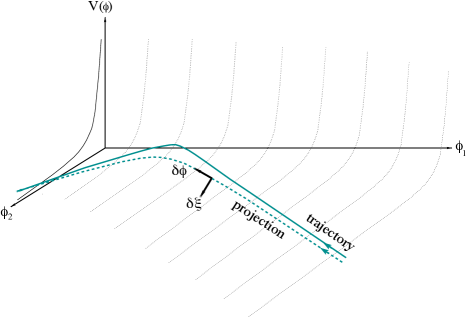
IV.5.4 Non-Gaussianities in other proposals
A model which does not generate large intrinsic non-Gaussianities is that based on a non-minimal entropic mechanism Fertig et al. (2014); Ijjas et al. (2014b), following the model introduced in Qiu et al. (2013); Li (2013). It employs a second scalar, which does not contribute to the potential, but is non-minimally coupled to the ekpyrotic scalar in its kinetic function. In contrast to standard entropic mechanisms, there are no non-Gaussianities generated during the ekpyrotic phase at leading order. The authors evaluate the contribution to curvature perturbations sourced by entropy perturbations at second order within different phases: first, the contribution to the curvature perturbation from entropy perturbations during the ekpyrotic phase – these are non-existent; second, the introduction of a time-varying equation of state, as required to end the ekpyrotic phase, gives perfectly Gaussian entropy perturbations and vanishing curvature perturbations; third, a conversion from entropy to curvature perturbations, including a bend in the trajectory at the end of the ekpyrotic phase, or a conversion at the bounce via modulated (p)reheating. The magnitude of non-Gaussianities is dependent on the non-linearity of the conversion mechanism, as explained in the previous sections, and thus model dependent, but it can be below the bounds imposed by PLANCK.
Non-Gaussianities in a nonsingular matter bounce were studied in Cai et al. (2009a). The matter bounce referred to here deals with fluctuations generated as quantum vacuum perturbations which exit the Hubble radius during a matter-dominated contracting phase Finelli and Brandenberger (2002); Wands (1999); Allen and Wands (2004); Peter and Pinto-Neto (2008). The amplitude and shape of the three-point function is computed. The local non-linearity parameter arising from the adiabatic mode is . Its large value, compared to inflationary predictions, is caused by the growth of adiabatic fluctuations after Hubble crossing during the contracting phase. As with the perturbation spectrum itself, in order to compare the non-Gaussianities, here calculated in the contracting phase, with actual observations, one needs to evaluate how they pass through the bounce itself. This is the subject of the following section.
IV.6 Getting perturbations through a bounce
In order to agree with observations, it is often assumed that a nearly scale-invariant spectrum of curvature perturbations is generated during the contracting phase; in Sec. IV.2 we discussed several possible ways to generate such a scale-invariant spectrum. However, the question remains whether it emerges unscathed after the bounce.
After Hubble crossing, is frozen, at least as long as the evolution takes place during an adiabatic regime. However, as the bounce is approached, modes become sub-Hubble again between and , see Fig. 5 and Fig. 20; during this interval, modes can evolve in a way that differs from their “frozen” super-Hubble evolution, requiring a careful analysis of the perturbations during the actual bounce. If the bounce is fast enough, the naive intuition that perturbations are left unchanged can be correct, but counter examples exist (and in particular, the idea according to which scales larger than the bounce duration cannot be affected for “causality” reasons is wrong, as the horizon is made much larger than any relevant scale Martin and Peter (2004a)).
To illustrate possible stumbling blocks, consider the original ekpyrotic scenario Khoury et al. (2002b) as a case study, where it was shown that the Bardeen potential inherits a scale-invariant spectrum, and it was argued that it remains unaltered during the bounce Khoury et al. (2002b). This argument was based on the fact that the dominant mode303030In an expanding or contracting universe, the second order differential equation of a perturbation variable has two solutions, a dominant and a sub-dominant one, the latter, by definition, becoming less and less important as time progresses. This is not always the case, as discussed in Sec. V. of the Bardeen potential carries the desired spectrum. In this scenario the pre- and post-bounce solutions are glued together at some hypersurface. The resulting matching conditions in Khoury et al. (2002b) were criticized in Martin et al. (2003). If one employs the Deruelle-Mukhanov matching conditions Deruelle and Mukhanov (1995); Hwang and Vishniac (1991) on a constant field hypersurface, one finds that the dominant mode in the contracting phase only couples to the sub-dominant one after the bounce Brandenberger and Finelli (2001). See also Hwang (2002); Tsujikawa (2002). As a consequence, as we have seen in Sec. IV.2.2, the curvature fluctuation inherits a blue spectrum Lyth and Wands (2002).
Evidently, the resulting spectrum depends crucially on the type of matching surface Durrer and Vernizzi (2002). In addition, some variables may become singular, as pointed out in Lyth (2002b), see Sec. IV.1.
In a nonsingular bounce, certain variables may still grow sufficiently large as to eventually behave in a non-perturbative way, but the resulting spectrum of cosmological fluctuations is at least in principle unambiguous: one simply needs to follow a well-behaved fluctuation variable throughout the bounce (or perform a non-perturbative analysis). In general, the curvature fluctuation after the bounce inherits components from both modes, dominant and sub-dominant, of the contracting phase in varying degrees. The detailed form of this mode mixing matrix is model dependent, see Martin and Peter (2003, 2004b); Bozza and Veneziano (2005).
This problem does not arise for tensor modes since those always remain below their potential, i.e. , as shown in Eq. (140) and Fig. 5. Thus, the spectrum of gravitational waves is largely insensitive to the bounce.
In the next section we discuss potentially dangerous instabilities, in particular the possible regrowth of the sub-dominant mode during the contracting phase in specific models.
V Potentially fatal effects undermining nonsingular models
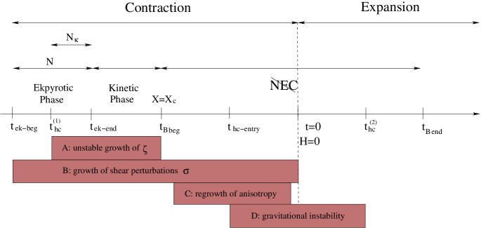
We follow Xue and Steinhardt (2010, 2011); Xue (2014) to investigate four effects that can undermine the success of nonsingular models:
-
A.
unstable growth of curvature fluctuations in the adiabatic mode,
-
B.
growth of quantum induced anisotropy for vector perturbations and scalar shear,
-
C.
regrowth of initial anisotropy as sub-dominant modes become dominant,
-
D.
gravitational instability during the bounce,
Throughout this section, we work in the framework of the new ekpyrotic scenario as a concrete case study and use the following notation: is the kinetic function, , is the kinetic energy, and a subscript “c” as in denotes the ghost condensate point. We assume that the ghost condensation occurs for small , so that the kinetic energy is vastly smaller during the bounce than at the end of the ekpyrotic phase. A subscript denotes any time during the bounce, and are the adiabatic curvature perturbation and the curvature perturbation generated via the entropic mechanism respectively. We call the number of e-folds of ekpyrosis left after the mode with wavenumber has crossed the Hubble radius and is the total number of e-folds during the ekpyrotic phase. The shear is : is the vector perturbation arising from the shear perturbation and is the scalar part of the shear in the synchronous gauge. The beginning and end of a bounce phase are represented respectively as and . Similarly, “” and “” denote the beginning and end of the ekpyrotic phase, while and denote the beginning and end of the bouncing phase. In Xue and Steinhardt (2011), the instabilities are considered only in the contracting phase. Our notation differs from Xue and Steinhardt (2011) as we consider contraction and expansion. The reader should take note that some of these problems can be avoided if ghost condensation occurs for large , as in the matter bounce model described in Sec. III.3.3.
V.1 Unstable growth of curvature fluctuations
The potentially unstable growth of curvature perturbations in nonsingular bouncing models may endanger their validity Xue and Steinhardt (2010, 2011). This threat comes in the form of a subdominant adiabatic mode that crosses its potential before the ekpyrotic phase is over, grows exponentially and ultimately gives rise to a blue spectrum, precluding the scale-invariant contribution to the temperature fluctuations in the CMBR. To see how this happens, we want to compare the resulting adiabatic perturbations to the isocurvature ones, by calculating the evolution of in the transition phase between the ekpyrotic and the bouncing one. The comoving curvature perturbations , labeled by the comoving wave number , obey the equations of motion,
| (156) |
where . The sound speed is
| (157) |
For small , the solution to (156) is
| (158) |
where and ; the first term of (158) is a constant solution with a blue spectrum; the second one is a decaying solution with a bluer spectrum and always ignored. Following Xue and Steinhardt (2010, 2011) we look at the second, integral term to show how this initially sub-dominant term can be amplified to eventually dominate over isocurvature perturbations; plugging in , we have
| (159) |
Using (157) along with and as detailed in Xue and Steinhardt (2011), the adiabatic contribution to the curvature perturbation
| (160) |
is greatly amplified. The ratio of this mode to the curvature perturbation produced via the entropic mechanism is
| (161) |
where is the number of e-folds of ekpyrosis left after the mode with wavenumber has crossed the Hubble scale and is the total number of e-folds during the ekpyrotic phase.
Since for modes observable in the CMBR, this regrowth of perturbations can be problematic for . One might hope to alleviate this problem by making exponentially large; however, this is impossible for modes observed in the CMBR due to the COBE normalization, see (173) where the exponential ekpyrotic potential in (26) is used. Other solutions to this problem must therefore be found.
V.2 Growth of quantum induced anisotropy
Starting with a homogeneous universe, do vector perturbations and scalar shear perturbations generated by quantum fluctuations dominate the energy density and prevent a nonsingular bounce? Under approximations made specifically for a bounce generated via a ghost condensate, namely, that both , the kinetic energy and are monotonically decreasing, and as well as , the Friedmann equations during the bouncing phase
| (162) | |||||
| (163) |
show that indeed it would be hard to get rid of shear perturbations . The potential energy at which the NEC is violated is denoted by and is the kinetic term. Assuming that and thus is monotonically decreasing during the bounce, one can derive a necessary condition for a ghost condensate to occur by requiring that vanishes at some point. Taking into account anisotropy one needs to have,
| (164) |
for some time during the bounce. If this bound is satisfied, the BKL-unstable behavior is avoided and a smooth bounce results, whereas a violation most likely indicates a failed bounce. It is expected that a similar condition has to be satisfied for any type of nonsingular bounce Xue and Steinhardt (2011).
To investigate sources of anisotropy, consider the general perturbed metric, containing vector and tensor modes as well as scalars,
| (165) | |||||
There are two common ways in which anisotropies arise Xue and Steinhardt (2011). The first stems from non-zero, gauge-invariant vector perturbations arising from the shear perturbation at constant time hypersurfaces,
| (166) |
which grow as the scale factor decreases during the ekpyrotic phase as Battefeld and Brandenberger (2004)
| (167) |
However, if we start with a universe initially devoid of vector perturbations and only scalars are present, this hurdle can be overcome as scalars do not source vector perturbations Battefeld and Brandenberger (2004). This is possible as vector perturbations, not being dynamical in this context, do not need to have non-vanishing initial conditions coming from, e.g. quantum vacuum fluctuations. The second source of anisotropies is due to the equation of state parameter passing through . The scalar part of the shear perturbation is
| (168) | |||||
Unlike , is not gauge invariant and its evolution is coupled to the comoving curvature pertubation . This would imply that the comoving shear and curvature perturbations feed off each other and grow from quantum fluctuations. However, in the synchronous gauge, and the shear perturbation stay small throughout the contracting phase till near the bounce. The comoving and synchronous shear perturbations, and , are related, so that one can translate one to the other Xue and Steinhardt (2011).
In the synchronous gauge313131The subscript denotes the synchronous gauge, whereas, the superscript denotes the scalar part of the shear. one obtains
| (169) |
which shows similar growth as the shear from vector perturbations in (167). Since scalar shear perturbations are continuously sourced during the contraction, this shear cannot be fined tuned away. A lower estimate of the shear anisotropy at the end of the bounce can be computed via the self-correlation function of integrated from modes that are deeply blue to modes that are above their potential till near the bounce Xue and Steinhardt (2011),
| (170) |
Here, denotes the turnaround between contraction and expansion. Consider a case study where the bounce is produced via a ghost condensate. In order to overcome the anisotropy, the condition for a bounce within this model is (164), which requires that
| (171) |
which can be satisfied only if (recall we are using units in which the reduced Planck mass is unity)
| (172) |
This value is in contradiction with the potential energy required by COBE at the ekpyrotic phase Lehners et al. (2007a),
| (173) |
where sets the exponent of the ekpyrotic potential in (26) Khoury et al. (2003). As such, the anisotropy arising from the scalar shear can dominate the energy density before the bounce, leading to BKL-like contractions, and prevent a bounce.
Working in the synchronous gauge, the computation stays perturbative (in contrast to the comoving gauge perturbation calculation), but the final result is still gauge dependent. In Xue and Steinhardt (2011) it was checked that the bounce is spoiled in two other gauges, the uniform Hubble gauge and the longitudinal gauge. In the latter, shear is absent, but the bounce is still spoiled by the appearance of large velocity perturbations. Hence, although it appears that this problem is physical, a full gauge-invariant computation has not been performed yet, so no definite conclusion can be drawn.
V.3 Regrowth of initial anisotropy
A detailed analysis of a ghost condensate-mediated bouncing phase in Xue and Steinhardt (2010, 2011); Xue (2014) shows that the initial anisotropy originally quelled during the ekpyrotic phase overtakes the scalar field energy when during the bouncing phase. Following the ekpyrotic phase, the curvature and anisotropy are suppressed by
| (174) |
To quantify the duration of the bounce, Xue et al. Xue and Steinhardt (2011) studied three different stages: at the beginning of the bounce the kinetic energy is negligible and . Subsequently, the friction term becomes dominant due to an increase in the negative kinetic energy. Close to the bounce , but since the Hubble rate is small, friction is again negligible. Of these three phases, the first and third ones are brief. Thus, the duration of the bounce phase can be approximated by
| (175) |
where . This result shows that it is not possible to complete the bounce in just a few Hubble times, leading to a growth of anisotropies. Hence, the scale factor scales as
| (176) |
and it contracts as
| (177) |
Therefore anisotropies increase by a factor of
| (178) |
which cancel the original anisotropy suppression experienced during ekpyrotic phase (174). As such, anisotropy persists, undermining the bouncing phase of the model at hand, unless the initial anisotropy is fine-tuned to,
| (179) |
This regrowth of anisotropy appears generic in models containing a prolonged friction-dominated phase with as evident from equations (177) and (178). See section III.1.5 for an example of how the cyclic universe eradicates the initial anisotropy via the presence of a Dark Energy phase before the ekpyrotic one.
V.4 Gravitational instability
During the bounce, modes re-enter the Hubble sphere briefly, where they may grow unstable if . The latter is not a necessary condition for a bounce to occur, but it is often the case. The presence of an instability becomes evident by considering the equation of motion of the Mukhanov-Sasaki variable
| (180) |
where . If we let
| (181) |
then
| (182) |
can be solved to
| (183) |
The resulting instability could be alleviated if were sufficiently small and/or the bounce duration in conformal time were not too large.
For a bounce mediated via a ghost condensate, the time interval inside the Hubble radius,
| (184) |
represents a problem for modes with . Hence to avoid the instability, the speed of sound has to be
| (185) |
VI Topics for future research interest
The attempts to investigate bouncing cosmologies as an alternative to the inflationary paradigm have been riddled with difficulties, roadblocks and no-go theorems. As a consequence, models have become rather complicated to avoid the many pitfalls. Nevertheless, use of newly proposed ingredients such as galileons or string gases have led to a few models that, although not free of problems, appear promising and thus offer some hope.
We hope to have given a critical, yet unbiased assessment of failures and successes. Focusing on the few surviving candidates, again all based on a classical description of gravity, we would like to outline a possible road-map for future research that might be of interest to scientists working on bouncing cosmologies.
VI.1 Preheating and reheating
The nature of reheating the early Universe is an active area of research in inflationary cosmology with a long history Kofman et al. (1997); Bassett et al. (2006). See for example Meyers and Tarrant (2013) for recent work on perturbative reheating after multi-field inflation and Zhang et al. (2013); Underwood and Zhai (2013) for preheating in DBI inflation. Reheating is a process whereby the cold post-inflationary universe attains the high temperature needed for nucleosynthesis. The inflaton decay can occur either perturbatively or via instabilities and/or resonances as in preheating. Perturbative reheating is almost always hampered by the incomplete decay of the inflaton which may spoil nucleosynthesis Braden et al. (2010). Most studies of preheating focus on canonical scalar fields Battefeld and Kawai (2008); Battefeld (2008), but little attention has been paid to the decay of non-standard fields such as scalars with more general kinetic terms or galileons, among others. Notable exceptions are a study of preheating in DBI inflation based on lattice simulations Child et al. (2013) as well as the rapid decay of a galileon in galileon genesis Perreault Levasseur et al. (2011). Another focus has been reheating in Starobinsky’s model of -inflation Starobinsky (1980); Rudenok et al. (2014) as well as in models of Higgs inflation Mazumdar and Rocher (2011) and the MSSM Allahverdi et al. (2010).
In the framework of cosmic bounces, this phase has hardly been studied at all, since the bounce physics itself was poorly understood. Early ideas entail the transfer of kinetic energy during the brane collision in singular ekpyrotic models Steinhardt and Turok (2002); Lehners (2011b), the transfer of the ghost condensate potential energy due to a steep drop of the potential and the assumed coupling to other degrees of freedom in new ekpyrosis Buchbinder et al. (2007a), or the application of inflationary reheating/preheating lore after a bounce Battefeld (2008). In the context of a nonsingular bounce with a matter dominated contracting phase caused by an oscillating scalar field, stochastic resonance, i.e. preheating, was studied in Cai et al. (2011b), where it was shown that preheating can be more efficient: resonances can commence in the contracting, matter dominated phase and continue throughout the bounce, in effect doubling the period of preheating. However, only canonical scalar fields were considered for preheating dynamics, leaving the NEC violating field out of this process. In the framework of a singular bounce mediated by a brane collision, it was speculated that the presence of additional light degrees of freedom before a singular bounce would render the bounce nonsingular and reheat the universe subsequently via the intermediately produced light degrees of freedom. The S-brane bounce may be viewed as a realization of this idea.
While several mechanisms to generate a nearly scale-invariant spectrum of perturbations are known, and models differ in this regard, we have encountered only two distinct avenues of inducing a nonsingular classical bounce without introducing fatal instabilities (but not entirely devoid of problems):
- 1.
- 2.
In either case, (p)reheating has not been studied, but it is possible to identify the challenges ahead.
In the first case (employing galileons/ghost condensates), it is necessary to ensure that any coupling to matter fields does not lead to a premature decay of the bounce-inducing ingredient, while ensuring that it decays sufficiently before nucleosynthesis. Since it is unknown if preheating dynamics are operational for galileons, studies investigating preheating should be conducted, including lattice simulations if preheating is feasible. Further, in the presence of additional isocuvature fields that carry the scale-invariant spectrum, their decay products have to dominate over the galileon’s. Once a better understanding of the thermal history is available, the presence of thermal relics and the effect onto non-Gaussianities will have to be investigated.
In the second case, a thermal component, a string gas modeled by a scalar in the S-brane bounce, is present, with a temperature close to the Hagedorn one. Naively, one should expect the production of a large number of different particle species in this regime, not only standard model ones. Thus, it is crucial to identify mechanisms that predominately lead to standard model particles after the bounce. The production of thermal relics, such as gravitinos, at these high temperatures is an example of this challenge, see Sec. III.1.4. In addition, while it can be argued that the thermal string gas may be modeled by a scalar field at the background and even the perturbed level, it is probably an oversimplification to use such a setup to discuss (p)reheating dynamics, much like effective single field models of inflation are insufficient to study preheating Battefeld and Kawai (2008).
Evidently, reheating emerges as one of the most challenging and ill-understood regimes of bouncing cosmologies, even more so than in inflationary setups, offering many new challenges for future research.
VI.2 An implementation within string theory
Great advances have been made to implement inflationary cosmology in string theory, see. e.g. Cline (2006); McAllister and Silverstein (2008); Burgess and McAllister (2011); Baumann and McAllister (2014) for reviews. Crucial components of any implementation are the identification of the dynamical degrees of freedom with their microphysical counterparts, such as a brane separation turning into an inflaton, as well as a thorough understanding of moduli stabilization323232For a recent assessment on moduli stabilization in Type IIB string theory, see Dasgupta et al. (2014), where necessary conditions at the full D level were derived., such as the shape and size of extra dimensions. The inflaton potential’s sensitivity to quantum corrections emerged as a roadblock for many setups, which led to a preference of small field models or highly symmetric scenarios such as monodromy inflation Silverstein and Westphal (2008).
For bouncing cosmologies we are just at the beginning stages of finding implementations within string theory. Since galileon models emerged over the last few years as promising phenomenological candidates to provide a well-behaved cosmological bounce, the logical next step should be to find concrete realizations of galileons in string theory. In that regard the construction of a supersymmetric version of a galileon setup as provided in Koehn et al. (2014) is encouraging. Furthermore, once methods of realizing galileons in string theory are found, suitable potentials have to be devised. Only after such an implementation is found can questions pertaining to moduli stabilization or quantum corrections be addressed. However, these models do not generate measurable primordial gravitational waves on CMBR scales and would therefore be ruled out if the BICEP2 result stands the test of time and no additional mechanism to generate gravitational waves is present.
A model incorporating stringy degrees of freedom to generate a bounce has been proposed in Brandenberger et al. (2013) (the S-brane bounce) making use of a string gas. Here the main simplification consists of a gas approximation, which is further approximated by modeling the thermal string gas by a scalar field. Furthermore, the study stayed at the level of the 4D effective theory. All of these approximations should be relaxed. In the framework of string gas cosmology, the dynamics of toroidal internal dimensions can be discussed in the framework of dilaton gravity Battefeld and Watson (2004). However, since the bounce takes place in the Hagedorn regime, any discussion of moduli stabilization is daunting333333It has been proposed to use the string gas to stabilize internal dimensions as well as the dilaton Patil and Brandenberger (2005, 2006); Patil (2005); Danos et al. (2008); Mishra et al. (2012), see also Watson and Brandenberger (2003); Watson (2004); Brandenberger et al. (2006b); Cremonini and Watson (2006); Liu and Partouche (2012). This proposal works within dilaton gravity and is not necessarily valid in the Hagedorn regime. Furthermore, since string gases redshift like matter, this stabilization mechanism is problematic at late times Battefeld and Shuhmaher (2006), particularly in the presence of a cosmological constant Ferrer and Rasanen (2006)..
If bouncing cosmology is to provide an alternative to the inflationary paradigm, and if string theory is the correct way to describe physics at the highest energy level, then considerable improvements have to be made to implement them in string theory. To this end, a resolution of the singularity should take center-stage. Only if such a resolution is achieved will we be able to assess whether a galileon bounce, a string gas bounce, or a singular antigravity bounce can provide a good description of the early Universe.
VI.3 Spatial curvature and non-Gaussianities
Spatial curvature is often neglected, and indeed, we mostly assumed throughout this review. The usual argument for this choice, apart from the observational fact that curvature is negligible today, is that it should not dominate during a bouncing phase. The equivalent energy density being , curvature is always subdominant in the Friedmann Eqs. (6) when compared to dust (), radiation () and in particular the shear (), as discussed in Sec. III.2.1, when . Now let the energy density near the bounce consist in two pieces, and say, where denotes the component whose negative contribution during the bouncing phase allows for the bounce to actually take place in the framework of GR. The Friedmann equation for the background (6), if valid until the bounce, shows two possibilities: either , in which case the curvature contribution is indeed negligible at all times, including the bounce itself, or , i.e. all terms are of the same order of magnitude. In the latter case, the curvature contribution cannot be neglected, and the Friedmann equation then serves to determine the actual value of the scale factor at the bounce. Although perhaps very contrived and fine-tuned, this is the case we now consider for the sake of completeness.
Even though it can be written as a perfect fluid with equation of state parameter in the background equations, curvature is actually not a fluid and cannot be perturbed; as a consequence, it does not entail any dynamical degrees of freedom at the perturbed level, but if , conservation laws, such as that of the curvature perturbation , are not generically valid. As a consequence, new variables should be considered instead, such as the BST curvature variable Wands et al. (2000): although the “pure” curvature perturbation is no longer conserved in the presence of spatial curvature, the new quantity, which reduces to the former in the limit , can be conserved on super Hubble scales under specific conditions which do not necessarily hold in a bouncing scenario Abramo and Peter (2007); Martin and Peter (2004a). One can note at this point that in the so-called bounce scenario in Abramo and Peter (2007), for instance, the bounce is explicitly performed in a spatially curved universe, the limit being assumed regular; it might not necessarily be a valid assumption depending on the specific form of the action De-Santiago et al. (2013).
How spatial curvature can drastically modify a model’s prediction is illustrated in Martin and Peter (2003); Falciano et al. (2008): here, a simple bouncing model is considered, based on a scalar field and curvature. The former has a potential whose maximum is reached at the bounce, which is canceled by the curvature contribution, such that without violating the NEC. As a result, many instabilities are avoided by construction. The effective potential entering the equations of motion for perturbations is strongly model-dependent. Furthermore, the amplitude and the spectral index of curvature fluctuations strongly depend on dynamics during the bounce. Thus, the mere presence of a curvature term can imply that the observed spectrum is not necessarily the one produced during the contracting phase.
The situation can be even more problematic if non-linear terms in the perturbative expansion are considered: for the same model, an almost de Sitter bounce can be a strong producer of non-Gaussianities, as shown by one of the authors of this review and collaborators in Gao et al. (2014b). As a result, the prediction of non-Gaussianities based on pre-bounce physics, as in Cai et al. (2009a), may not be sufficient. The latter would indicate that non-Gaussianities from the matter bounce are usually small, while the former would predict exactly the opposite.
As we have seen, curvaton-like models already produced reasonably large non-Gaussianities from the conversion mechanism. If their amplitude remains unaffected by the bounce physics, they can still be affected by the subsequent phase of (p)reheating, which can change not only the amplitude but also the sign of non-linearity parameters Leung et al. (2012, 2013); Elliston et al. (2014). Thus, as highlighted above, a thorough understanding of preheating is essential for any comparison of predictions with current and forthcoming high-precision data.
VI.4 Primordial gravitational waves
Primordial gravitational waves have been propagating undisturbed to us since their formation and particularly after decoupling, some years after the big bang. On their way, they have imprinted a particular signal on the CMBR, which induces vorticity in the polarization field. This polarization pattern consists of a B-mode component at angular degree that cannot be generated by primordial density perturbations. The amplitude of this signal is given by the tensor to scalar ratio, , a function of the energy scale of inflation. The BICEP2 experiment Ade et al. (2014a) claims to have observed such gravitational waves, and if the interpretation of this result is confirmed independently by other experiments at different frequencies and on different patches on the sky, this would support inflation as the standard paradigm of the early Universe, see Sec. IV.4 for a summary of the ongoing debate. Indeed, inflation predicts gravitational waves with amplitudes determined by the energy scale at which inflation happened Bassett et al. (2006); Starobinskii (1979),
| (186) |
where is the energy density at the time of inflation. Hence, according to this observation, inflation took place around the GUT scale. In addition, however, via the Lyth bound Lyth (1997), the arc length of the inflationary trajectory would have to be super-Planckian
| (187) |
thus potentially raising theoretical questions regarding the use classical GR at this stage.
As we have seen in Sec. IV.3, the primordial gravitational wave spectrum generated during an ekpyrotic phase, that is a slow contraction, is blue with a strongly suppressed amplitude. Since all of the promising proposals include such a contracting phase, with the exception of the S-brane bounce and the Hagedorn bounce by T-duality in string gas cosmology, see Sec. III.3.5, they would be ruled out in the absence of any additional mechanism to yield such a primordial gravitational wave spectrum. While an ekpyrotic phase was not incorporated in the S-brane bounce, the latter suffers from instability problems, see Sec. III.2.2, exactly due to the absence of an ekpyrotic phase. If we ignore these problems and focus on a matter dominated contracting phase, see Sec. IV.2.4, the spectrum of gravitational waves is scale invariant but can be in excess of current bounds Allen and Wands (2004); Cai et al. (2009b). Thus, only a few models are potentially in agreement with the BICEP2 experiment: the string gas model (the Hagedorn bounce, not the S-brane bounce) sketched in Sec. III.3.5 (see however Kaloper et al. (2006)), the matter bounce curvaton Cai et al. (2011c) and the new matter bounce Cai et al. (2014), since they can accommodate the indicated amplitude of gravitational waves. String gas cosmology also predicts that the tensor spectral index is blue, opposite to the red one in inflationary cosmology, so that one may be able to discriminate between these frameworks. The Hagedorn bounce however has its own problems for the reasons previously discussed (flatness, relic problem, etc. ).
All in all, it appears that most classical gravity based bouncing models might be in trouble for one reason or another (e.g. the observed red tilt in the spectrum, the lack of non-Gaussianities, primordial tensor modes, some questions of stability and background compatibility), so that the search for a complete model is ongoing. Quantum gravity effects, viewed from this perspective, could provide more effective solutions in the future.
To alleviate the difficulties highlighted in this review often requires complicating the model. The fact that a working model is complicated does not necessarily mean that it is incorrect vis-à-vis the way the Universe actually evolved; although Ockham’s razor demands that we look for a simple theoretical framework, it does not imply that a model’s veracity relies on its simplicity. For example, as Copernicus proposed the heliocentric model in lieu of Ptolemic’s geocentric one, he included more epicycles due to his insistence on using circular orbits. Thus, his model could have been the victim to Ockham’s razor. Only subsequent improvements to his model, particularly the use of ellipses, led to the simple Keplerian model we know today, which is still an approximation to the full solution in General Relativity. Bouncing cosmologies may be at a similar stage, where simplicity, if present, is not yet apparent. Thus, we should strive to extract distinct predictions of bouncing cosmologies and confront them with experiments, while simultaneously aiming to improve the conceptual underpinning. We hope the present review of pros and cons can be helpful in achieving these goals.
Acknowledgments
It is a pleasure to thank Thorsten Battefeld, Martin Bojowald, Robert Brandenberger, Yi-Fu Cai, Jean-Luc Lehners, Andrei Linde, Luboš Motl, Jérôme Martin, Hermann Nicolai, Suboth Patil, Nelson Pinto-Neto, Paul Steinhardt, Sandro Vitenti and BinKan Xue for comments, suggestions and discussions. We would also like to thank Mónica Forte, Miguel Sousa Costa, Jorge Luis Cervantes Cota, Anupam Mazumdar, Marco Peloso, Yun-Song Piao, Parampreet Singh, Martin S. Sloth and Gregory Vereshchagin for comments on the draft.
References
- Mukhanov (2005) V. Mukhanov, Physical foundations of cosmology (Cambridge University Press, 2005).
- Peter and Uzan (2009) P. Peter and J.-P. Uzan, Primordial cosmology, Oxford Graduate Texts (Oxford University Press, Oxford, 2009).
- Ade et al. (2014a) P. Ade et al. (BICEP2 Collaboration), Phys.Rev.Lett. 112, 241101 (2014a), eprint 1403.3985.
- Guth (1981) A. H. Guth, Phys. Rev. D23, 347 (1981).
- Ijjas et al. (2013) A. Ijjas, P. J. Steinhardt, and A. Loeb, Phys. Lett. B723, 261 (2013), eprint 1304.2785.
- Ijjas et al. (2014a) A. Ijjas, P. J. Steinhardt, and A. Loeb (2014a), eprint 1402.6980.
- Linde (2008) A. D. Linde, Lect. Notes Phys. 738, 1 (2008), eprint 0705.0164.
- Lemoine et al. (2008) M. Lemoine, J. Martin, and P. Peter, Lect. Notes Phys. 738 (2008).
- Baumann (2009) D. Baumann (2009), eprint 0907.5424.
- Martin et al. (2014a) J. Martin, C. Ringeval, and V. Vennin, Phys.Dark Univ. (2014a), eprint 1303.3787.
- Martin et al. (2014b) J. Martin, C. Ringeval, R. Trotta, and V. Vennin, JCAP 1403, 039 (2014b), eprint 1312.3529.
- Baumann and McAllister (2014) D. Baumann and L. McAllister (2014), eprint 1404.2601.
- Guth et al. (2014) A. H. Guth, D. I. Kaiser, and Y. Nomura, Phys.Lett. B733, 112 (2014), eprint 1312.7619.
- Linde (2014) A. Linde (2014), eprint 1402.0526.
- Barrow and Liddle (1997) J. D. Barrow and A. R. Liddle, Gen.Rel.Grav. 29, 1503 (1997), eprint gr-qc/9705048.
- Ringeval et al. (2007) C. Ringeval, M. Sakellariadou, and F. Bouchet, JCAP 0702, 023 (2007), eprint astro-ph/0511646.
- Peter and Ringeval (2013) P. Peter and C. Ringeval, JCAP 1305, 005 (2013), eprint 1302.0953.
- Ade et al. (2013a) P. Ade et al. (Planck Collaboration) (2013a), eprint 1303.5085.
- Battefeld and Watson (2006) T. Battefeld and S. Watson, Rev. Mod. Phys. 78, 435 (2006), eprint hep-th/0510022.
- Brandenberger et al. (2014) R. H. Brandenberger, A. Nayeri, and S. P. Patil, Phys.Rev. D90, 067301 (2014), eprint 1403.4927.
- Piao et al. (2004) Y.-S. Piao, B. Feng, and X.-m. Zhang, Phys.Rev. D69, 103520 (2004), eprint hep-th/0310206.
- Falciano et al. (2008) F. T. Falciano, M. Lilley, and P. Peter, Phys. Rev. D77, 083513 (2008), eprint 0802.1196.
- Lilley et al. (2011) M. Lilley, L. Lorenz, and S. Clesse, JCAP 1106, 004 (2011), eprint 1104.3494.
- Liu et al. (2013) Z.-G. Liu, Z.-K. Guo, and Y.-S. Piao, Phys.Rev. D88, 063539 (2013), eprint 1304.6527.
- Biswas and Mazumdar (2014) T. Biswas and A. Mazumdar, Class.Quant.Grav. 31, 025019 (2014), eprint 1304.3648.
- Hubble (1929) E. Hubble, Proc. Nat. Acad. Sci. 15, 168 (1929).
- Perlmutter et al. (1999) S. Perlmutter et al. (Supernova Cosmology Project), Astrophys. J. 517, 565 (1999), eprint astro-ph/9812133.
- Riess et al. (1998) A. G. Riess et al. (Supernova Search Team), Astron. J. 116, 1009 (1998), eprint astro-ph/9805201.
- Coc et al. (2014) A. Coc, J.-P. Uzan, and E. Vangioni, JCAP 1410, 050 (2014), eprint 1403.6694.
- Teyssier et al. (2009) R. Teyssier, S. Pires, S. Prunet, D. Aubert, C. Pichon, et al., Astron.Astrophys. 497, 335 (2009), eprint 0807.3651.
- Borde and Vilenkin (1996) A. Borde and A. Vilenkin, Int.J.Mod.Phys. D5, 813 (1996), eprint gr-qc/9612036.
- Martin et al. (2014c) J. Martin, C. Ringeval, R. Trotta, and V. Vennin, Phys.Rev. D90, 063501 (2014c), eprint 1405.7272.
- Flauger et al. (2014) R. Flauger, J. C. Hill, and D. N. Spergel, JCAP 1408, 039 (2014), eprint 1405.7351.
- Mortonson and Seljak (2014) M. J. Mortonson and U. Seljak, JCAP 1410, 035 (2014), eprint 1405.5857.
- Brandenberger et al. (1993) R. H. Brandenberger, V. F. Mukhanov, and A. Sornborger, Phys. Rev. D48, 1629 (1993), eprint gr-qc/9303001.
- Novello and Bergliaffa (2008) M. Novello and S. P. Bergliaffa, Phys. Rept. 463, 127 (2008), eprint 0802.1634.
- Lemaitre (1927) G. Lemaitre, Ann. Soc. Sci. Brux. Ser. I Sci. Math. Astron. Phys. A47, 49 (1927).
- Tolman (1931) R. C. Tolman, Phys. Rev. 38, 1758 (1931).
- Lemaître (1933) G. Lemaître, Ann. Soc. Sci. Brux. 53, 51 (1933).
- Lemaitre (1997) G. Lemaitre, Gen. Rel. Grav. 29, 641 (1997).
- Barrow and Dabrowski (1995) J. D. Barrow and M. P. Dabrowski, Mon.Not.Roy.Astron.Soc. 275, 850 (1995).
- Starobinskii (1978) A. A. Starobinskii, Sov. Astron. Lett. 4, 82 (1978).
- Starobinsky (1980) A. A. Starobinsky, Phys. Lett. B91, 99 (1980).
- Bassett et al. (2006) B. A. Bassett, S. Tsujikawa, and D. Wands, Rev. Mod. Phys. 78, 537 (2006), eprint astro-ph/0507632.
- Gasperini and Veneziano (2003) M. Gasperini and G. Veneziano, Phys. Rept. 373, 1 (2003), eprint hep-th/0207130.
- Durrer and Laukenmann (1996) R. Durrer and J. Laukenmann, Class. Quant. Grav. 13, 1069 (1996), eprint gr-qc/9510041.
- Peter and Pinto-Neto (2002a) P. Peter and N. Pinto-Neto, Phys. Rev. D65, 023513 (2002a), eprint gr-qc/0109038.
- Khoury et al. (2001a) J. Khoury, B. A. Ovrut, P. J. Steinhardt, and N. Turok, Phys. Rev. D64, 123522 (2001a), eprint hep-th/0103239.
- Martin and Peter (2003) J. Martin and P. Peter, Phys. Rev. D68, 103517 (2003), eprint hep-th/0307077.
- Xue and Steinhardt (2010) B. Xue and P. J. Steinhardt, Phys. Rev. Lett. 105, 261301 (2010), eprint 1007.2875.
- Deruelle and Mukhanov (1995) N. Deruelle and V. F. Mukhanov, Phys. Rev. D52, 5549 (1995), eprint gr-qc/9503050.
- Craps et al. (2012) B. Craps, T. Hertog, and N. Turok, Phys. Rev. D86, 043513 (2012), eprint 0712.4180.
- Craps et al. (2009) B. Craps, T. Hertog, and N. Turok, Phys. Rev. D80, 086007 (2009), eprint 0905.0709.
- Smolkin and Turok (2012) M. Smolkin and N. Turok (2012), eprint 1211.1322.
- Bars et al. (2011) I. Bars, S.-H. Chen, and N. Turok, Phys. Rev. D84, 083513 (2011), eprint 1105.3606.
- Bars (2011) I. Bars (2011), eprint 1109.5872.
- Bars et al. (2012) I. Bars, S.-H. Chen, P. J. Steinhardt, and N. Turok, Phys. Lett. B715, 278 (2012), eprint 1112.2470.
- Bars et al. (2014a) I. Bars, P. Steinhardt, and N. Turok, Phys. Rev. D89, 043515 (2014a), eprint 1307.1848.
- Bars et al. (2013) I. Bars, P. J. Steinhardt, and N. Turok, Phys. Lett. B726, 50 (2013), eprint 1307.8106.
- Bars (2012) I. Bars (2012), eprint 1209.1068.
- Bars et al. (2014b) I. Bars, P. Steinhardt, and N. Turok, Phys.Rev. D89, 061302 (2014b), eprint 1312.0739.
- Peter and Pinto-Neto (2002b) P. Peter and N. Pinto-Neto, Phys. Rev. D66, 063509 (2002b), eprint hep-th/0203013.
- Lin et al. (2011) C. Lin, R. H. Brandenberger, and L. Perreault Levasseur, JCAP 1104, 019 (2011), eprint 1007.2654.
- Qiu et al. (2011) T. Qiu, J. Evslin, Y.-F. Cai, M. Li, and X. Zhang, JCAP 1110, 036 (2011), eprint 1108.0593.
- Cai et al. (2007) Y.-F. Cai, T. Qiu, Y.-S. Piao, M. Li, and X. Zhang, JHEP 0710, 071 (2007), eprint 0704.1090.
- Kounnas et al. (2012a) C. Kounnas, H. Partouche, and N. Toumbas, Nucl. Phys. B855, 280 (2012a), eprint 1106.0946.
- Biswas et al. (2006) T. Biswas, A. Mazumdar, and W. Siegel, JCAP 0603, 009 (2006), eprint hep-th/0508194.
- Biswas et al. (2007) T. Biswas, R. Brandenberger, A. Mazumdar, and W. Siegel, JCAP 0712, 011 (2007), eprint hep-th/0610274.
- Langlois and Naruko (2013) D. Langlois and A. Naruko, Class. Quant. Grav. 30, 205012 (2013), eprint 1305.6346.
- Koehn et al. (2013a) M. Koehn, J.-L. Lehners, and B. Ovrut, Phys. Rev. D88, 023528 (2013a), eprint 1302.0840.
- Koehn et al. (2014) M. Koehn, J.-L. Lehners, and B. A. Ovrut, Phys.Rev. D90, 025005 (2014), eprint 1310.7577.
- Battarra et al. (2014) L. Battarra, M. Koehn, J.-L. Lehners, and B. A. Ovrut, JCAP 1407, 007 (2014), eprint 1404.5067.
- Smolin (2004) L. Smolin, Rev. Mod. Phys. pp. 655–682 (2004), eprint hep-th/0408048.
- Rovelli (2011) C. Rovelli, PoS QGQGS2011, 003 (2011), eprint 1102.3660.
- Nicolai et al. (2005) H. Nicolai, K. Peeters, and M. Zamaklar, Class. Quant. Grav. 22, R193 (2005), eprint hep-th/0501114.
- Henderson et al. (2013a) A. Henderson, A. Laddha, and C. Tomlin, Phys.Rev. D88, 044028 (2013a), eprint 1204.0211.
- Henderson et al. (2013b) A. Henderson, A. Laddha, and c. Tomlin, Phys. Rev. D88, 044029 (2013b), eprint 1210.3960.
- Tomlin and Varadarajan (2013) C. Tomlin and M. Varadarajan, Phys. Rev. D87, 044039 (2013), eprint 1210.6869.
- Atwood et al. (2009) W. Atwood et al. (LAT Collaboration), Astrophys. J. 697, 1071 (2009), eprint 0902.1089.
- Shao et al. (2010) L. Shao, Z. Xiao, and B.-Q. Ma, Astropart.Phys. 33, 312 (2010), eprint 0911.2276.
- Ackermann et al. (2009) M. Ackermann et al. (Fermi GBM/LAT Collaborations), Nature 462, 331 (2009), eprint 0908.1832.
- Aharonian et al. (2008) F. Aharonian et al. (H. E. S. S. Collaboration), Phys. Rev. Lett. 101, 170402 (2008), eprint 0810.3475.
- Abramowski et al. (2011) A. Abramowski et al. (HESS Collaboration), Astropart.Phys. 34, 738 (2011), eprint 1101.3650.
- Amelino-Camelia et al. (1998) G. Amelino-Camelia, J. R. Ellis, N. Mavromatos, D. V. Nanopoulos, and S. Sarkar, Nature 393, 763 (1998), eprint astro-ph/9712103.
- Vasileiou et al. (2013) V. Vasileiou, A. Jacholkowska, F. Piron, J. Bolmont, C. Couturier, et al., Phys. Rev. D87, 122001 (2013), eprint 1305.3463.
- Bojowald (2012) M. Bojowald, Class. Quant. Grav. 29, 213001 (2012), eprint 1209.3403.
- Ashtekar and Singh (2011) A. Ashtekar and P. Singh, Class. Quant. Grav. 28, 213001 (2011), eprint 1108.0893.
- Vereshchagin (2004) G. Vereshchagin, JCAP 0407, 013 (2004), eprint gr-qc/0406108.
- Singh et al. (2006) P. Singh, K. Vandersloot, and G. Vereshchagin, Phys.Rev. D74, 043510 (2006), eprint gr-qc/0606032.
- Cailleteau et al. (2009) T. Cailleteau, P. Singh, and K. Vandersloot, Phys.Rev. D80, 124013 (2009), eprint 0907.5591.
- Linsefors and Barrau (2013) L. Linsefors and A. Barrau, Phys. Rev. D87, 123509 (2013), eprint 1301.1264.
- Amorós et al. (2013) J. Amorós, J. de Haro, and S. D. Odintsov, Phys.Rev. D87, 104037 (2013), eprint 1305.2344.
- Mielczarek and Piechocki (2012) J. Mielczarek and W. Piechocki, Phys. Rev. D86, 083508 (2012), eprint 1108.0005.
- Gazeau et al. (2013) J. P. Gazeau, J. Mielczarek, and W. Piechocki, Phys. Rev. D87, 123508 (2013), eprint 1303.1687.
- Barrau et al. (2014) A. Barrau, T. Cailleteau, J. Grain, and J. Mielczarek, Class.Quant.Grav. 31, 053001 (2014), eprint 1309.6896.
- Wilson-Ewing (2013a) E. Wilson-Ewing, JCAP 1308, 015 (2013a), eprint 1306.6582.
- Gupt and Singh (2013) B. Gupt and P. Singh, Class.Quant.Grav. 30, 145013 (2013), eprint 1304.7686.
- Cai and Wilson-Ewing (2014) Y.-F. Cai and E. Wilson-Ewing, JCAP 1403, 026 (2014), eprint 1402.3009.
- Corichi and Vukasinac (2012) A. Corichi and T. Vukasinac, Phys.Rev. D86, 064019 (2012), eprint 1202.1846.
- Bojowald et al. (2009) M. Bojowald, G. M. Hossain, M. Kagan, and S. Shankaranarayanan, Phys. Rev. D79, 043505 (2009), eprint 0811.1572.
- Bojowald et al. (2008) M. Bojowald, G. M. Hossain, M. Kagan, and S. Shankaranarayanan, Phys. Rev. D78, 063547 (2008), eprint 0806.3929.
- Cailleteau et al. (2014) T. Cailleteau, L. Linsefors, and A. Barrau, Class.Quant.Grav. 31, 125011 (2014), eprint 1307.5238.
- Ashtekar et al. (2007) A. Ashtekar, T. Pawlowski, P. Singh, and K. Vandersloot, Phys. Rev. D75, 024035 (2007), eprint gr-qc/0612104.
- Ashtekar et al. (2006a) A. Ashtekar, T. Pawlowski, and P. Singh, Phys. Rev. D74, 084003 (2006a), eprint gr-qc/0607039.
- Ashtekar et al. (2006b) A. Ashtekar, T. Pawlowski, and P. Singh, Phys. Rev. Lett. 96, 141301 (2006b), eprint gr-qc/0602086.
- Wilson-Ewing (2013b) E. Wilson-Ewing, JCAP 1303, 026 (2013b), eprint 1211.6269.
- Shtanov and Sahni (2003) Y. Shtanov and V. Sahni, Phys. Lett. B557, 1 (2003), eprint gr-qc/0208047.
- Brown et al. (2008) M. G. Brown, K. Freese, and W. H. Kinney, JCAP 0803, 002 (2008), eprint astro-ph/0405353.
- Battefeld and Geshnizjani (2006) T. Battefeld and G. Geshnizjani, Phys. Rev. D73, 064013 (2006), eprint hep-th/0503160.
- Randall and Sundrum (1999) L. Randall and R. Sundrum, Phys. Rev. Lett. 83, 3370 (1999), eprint hep-ph/9905221.
- Bojowald and Paily (2012) M. Bojowald and G. M. Paily, Phys. Rev. D86, 104018 (2012), eprint 1112.1899.
- Singh (2012) P. Singh, Phys.Rev. D85, 104011 (2012), eprint 1112.6391.
- Thiemann (2007) T. Thiemann, Lect. Notes Phys. 721, 185 (2007), eprint hep-th/0608210.
- Holland (1993) P. Holland, Phys. Rept. 224, 95 (1993).
- Sanz and Miret-Artés (2012) A. S. Sanz and S. Miret-Artés, Lect. Notes Phys. 850, 187 (2012).
- Pinto-Neto and Fabris (2013) N. Pinto-Neto and J. Fabris, Class. Quant. Grav. 30, 143001 (2013), eprint 1306.0820.
- Acacio de Barros et al. (1998) J. Acacio de Barros, N. Pinto-Neto, and M. Sagioro-Leal, Phys. Lett. A241, 229 (1998), eprint gr-qc/9710084.
- Casadio (2000) R. Casadio, Int.J.Mod.Phys. D9, 511 (2000), eprint gr-qc/9810073.
- Peter et al. (2006) P. Peter, E. J. Pinho, and N. Pinto-Neto, Phys. Rev. D73, 104017 (2006), eprint gr-qc/0605060.
- Pinho and Pinto-Neto (2007) E. J. Pinho and N. Pinto-Neto, Phys. Rev. D76, 023506 (2007), eprint hep-th/0610192.
- Donagi et al. (2001) R. Y. Donagi, J. Khoury, B. A. Ovrut, P. J. Steinhardt, and N. Turok, JHEP 0111, 041 (2001), eprint hep-th/0105199.
- Khoury et al. (2001b) J. Khoury, B. A. Ovrut, P. J. Steinhardt, and N. Turok (2001b), eprint hep-th/0105212.
- Kallosh et al. (2001a) R. Kallosh, L. Kofman, and A. D. Linde, Phys. Rev. D64, 123523 (2001a), eprint hep-th/0104073.
- Kallosh et al. (2001b) R. Kallosh, L. Kofman, A. D. Linde, and A. A. Tseytlin, Phys. Rev. D64, 123524 (2001b), eprint hep-th/0106241.
- Lukas et al. (1999) A. Lukas, B. A. Ovrut, K. Stelle, and D. Waldram, Nucl.Phys. B552, 246 (1999), eprint hep-th/9806051.
- Martin et al. (2002) J. Martin, P. Peter, N. Pinto Neto, and D. J. Schwarz, Phys. Rev. D65, 123513 (2002), eprint hep-th/0112128.
- Martin et al. (2003) J. Martin, P. Peter, N. Pinto-Neto, and D. J. Schwarz, Phys. Rev. D67, 028301 (2003), eprint hep-th/0204222.
- Kragh (2013) H. Kragh (2013), eprint 1308.0932.
- Steinhardt and Turok (2002) P. J. Steinhardt and N. Turok, Phys. Rev. D65, 126003 (2002), eprint hep-th/0111098.
- Steinhardt and Turok (2001) P. J. Steinhardt and N. Turok (2001), eprint hep-th/0111030.
- Khoury et al. (2002a) J. Khoury, B. A. Ovrut, N. Seiberg, P. J. Steinhardt, and N. Turok, Phys. Rev. D65, 086007 (2002a), eprint hep-th/0108187.
- Felder et al. (2002) G. N. Felder, A. V. Frolov, L. Kofman, and A. D. Linde, Phys.Rev. D66, 023507 (2002), eprint hep-th/0202017.
- Mithani and Vilenkin (2012) A. Mithani and A. Vilenkin (2012), eprint 1204.4658.
- Brandenberger and Finelli (2001) R. Brandenberger and F. Finelli, JHEP 0111, 056 (2001), eprint hep-th/0109004.
- Lyth (2002a) D. H. Lyth, Phys.Lett. B524, 1 (2002a), eprint hep-ph/0106153.
- Durrer and Vernizzi (2002) R. Durrer and F. Vernizzi, Phys. Rev. D66, 083503 (2002), eprint hep-ph/0203275.
- Creminelli et al. (2005) P. Creminelli, A. Nicolis, and M. Zaldarriaga, Phys. Rev. D71, 063505 (2005), eprint hep-th/0411270.
- Tseng (2013) C.-Y. Tseng, Phys. Rev. D87, 023518 (2013), eprint 1210.0581.
- Battarra and Lehners (2014) L. Battarra and J.-L. Lehners, Phys.Rev. D89, 063516 (2014), eprint 1309.2281.
- Notari and Riotto (2002) A. Notari and A. Riotto, Nucl. Phys. B644, 371 (2002), eprint hep-th/0205019.
- Lehners et al. (2007a) J.-L. Lehners, P. McFadden, N. Turok, and P. J. Steinhardt, Phys. Rev. D76, 103501 (2007a), eprint hep-th/0702153.
- Buchbinder et al. (2007a) E. I. Buchbinder, J. Khoury, and B. A. Ovrut, Phys. Rev. D76, 123503 (2007a), eprint hep-th/0702154.
- Creminelli and Senatore (2007) P. Creminelli and L. Senatore, JCAP 0711, 010 (2007), eprint hep-th/0702165.
- Buchbinder et al. (2007b) E. I. Buchbinder, J. Khoury, and B. A. Ovrut, JHEP 0711, 076 (2007b), eprint 0706.3903.
- Kallosh et al. (2008) R. Kallosh, J. U. Kang, A. Linde, and V. Mukhanov, JCAP 4, 018 (2008), eprint 0712.2040.
- Woodard (2007) R. P. Woodard, Lect.Notes Phys. 720, 403 (2007), eprint astro-ph/0601672.
- Khoury et al. (2004) J. Khoury, P. J. Steinhardt, and N. Turok, Phys. Rev. Lett. 92, 031302 (2004), eprint hep-th/0307132.
- Khoury et al. (2002b) J. Khoury, B. A. Ovrut, P. J. Steinhardt, and N. Turok, Phys. Rev. D66, 046005 (2002b), eprint hep-th/0109050.
- Lehners and Steinhardt (2009) J.-L. Lehners and P. J. Steinhardt, Phys. Rev. D79, 063503 (2009), eprint 0812.3388.
- Lehners (2011a) J.-L. Lehners, Phys. Rev. D84, 103518 (2011a), eprint 1107.4551.
- Lehners (2008) J.-L. Lehners, Phys. Rept. 465, 223 (2008), eprint 0806.1245.
- Lehners and Steinhardt (2013) J.-L. Lehners and P. J. Steinhardt, Phys. Rev. D87, 123533 (2013), eprint 1304.3122.
- Lehners et al. (2009) J.-L. Lehners, P. J. Steinhardt, and N. Turok, Int. J. Mod. Phys. D18, 2231 (2009), eprint 0910.0834.
- Lehners (2011b) J.-L. Lehners, Class. Quant. Grav. 28, 204004 (2011b), eprint 1106.0172.
- Johnson and Lehners (2012) M. C. Johnson and J.-L. Lehners, Phys. Rev. D85, 103509 (2012), eprint 1112.3360.
- Enqvist and Sloth (2002) K. Enqvist and M. S. Sloth, Nucl.Phys. B626, 395 (2002), eprint hep-ph/0109214.
- Lyth and Wands (2002) D. H. Lyth and D. Wands, Phys. Lett. B524, 5 (2002), eprint hep-ph/0110002.
- Koyama et al. (2007a) K. Koyama, S. Mizuno, and D. Wands, Class. Quant. Grav. 24, 3919 (2007a), eprint 0704.1152.
- Koyama and Wands (2007) K. Koyama and D. Wands, JCAP 0704, 008 (2007), eprint hep-th/0703040.
- Koyama et al. (2007b) K. Koyama, S. Mizuno, F. Vernizzi, and D. Wands, JCAP 0711, 024 (2007b), eprint 0708.4321.
- Lehners et al. (2007b) J.-L. Lehners, P. McFadden, and N. Turok, Phys. Rev. D75, 103510 (2007b), eprint hep-th/0611259.
- Lehners et al. (2007c) J.-L. Lehners, P. McFadden, and N. Turok, Phys. Rev. D76, 023501 (2007c), eprint hep-th/0612026.
- Battefeld (2008) T. Battefeld, Phys. Rev. D77, 063503 (2008), eprint 0710.2540.
- Ade et al. (2014b) P. Ade et al. (Planck Collaboration), Astron.Astrophys. 571, A22 (2014b), eprint 1303.5082.
- Ade et al. (2013b) P. Ade et al. (Planck Collaboration) (2013b), eprint 1303.5083.
- Lehners and Steinhardt (2008a) J.-L. Lehners and P. J. Steinhardt, Phys. Rev. D77, 063533 (2008a), eprint 0712.3779.
- Lehners and Steinhardt (2008b) J.-L. Lehners and P. J. Steinhardt, Phys. Rev. D78, 023506 (2008b), eprint 0804.1293.
- Lehners (2010) J.-L. Lehners, Adv. Astron. 2010, 903907 (2010), eprint 1001.3125.
- Qiu et al. (2013) T. Qiu, X. Gao, and E. N. Saridakis, Phys. Rev. D88, 043525 (2013), eprint 1303.2372.
- Li (2013) M. Li, Phys. Lett. B724, 192 (2013), eprint 1306.0191.
- Fertig et al. (2014) A. Fertig, J.-L. Lehners, and E. Mallwitz, Phys.Rev. D89, 103537 (2014), eprint 1310.8133.
- Ijjas et al. (2014b) A. Ijjas, J.-L. Lehners, and P. J. Steinhardt (2014b), eprint 1404.1265.
- Xue and Belbruno (2014) B. Xue and E. Belbruno (2014), eprint 1403.2122.
- Saridakis (2009) E. Saridakis, Nucl. Phys. B808, 224 (2009), eprint 0710.5269.
- Biswas (2008) T. Biswas (2008), eprint 0801.1315.
- Novello et al. (2009) M. Novello, A. N. Araujo, and J. Salim, Int. J. Mod. Phys. A24, 5639 (2009), eprint 0802.1875.
- Medeiros (2012) L. Medeiros, Int.J.Mod.Phys. D23, 1250073 (2012), eprint 1209.1124.
- Sun (2008) C.-Y. Sun, Phys. Rev. D78, 064060 (2008), eprint 0806.1080.
- Son and Kim (2011) E. J. Son and W. Kim, Mod.Phys. Lett. A26, 719 (2011), eprint 1007.5371.
- Li et al. (2014) C. Li, L. Wang, and Y.-K. E. Cheung, Phys.Dark Univ. 3, 18 (2014), eprint 1101.0202.
- Sahni and Toporensky (2012) V. Sahni and A. Toporensky, Phys. Rev. D85, 123542 (2012), eprint 1203.0395.
- Stavrinos and Vacaru (2013) P. C. Stavrinos and S. I. Vacaru, Class. Quant. Grav. 30, 055012 (2013), eprint 1206.3998.
- Ivanov and Prodanov (2012) R. I. Ivanov and E. M. Prodanov, Phys. Rev. D86, 083536 (2012), eprint 1210.0186.
- Gao et al. (2014a) C. Gao, Y. Lu, and Y.-G. Shen, Gen.Rel.Grav. 46, 1791 (2014a), eprint 1402.3863.
- Barrow et al. (2004) J. D. Barrow, D. Kimberly, and J. Magueijo, Class.Quant.Grav. 21, 4289 (2004), eprint astro-ph/0406369.
- Clifton and Barrow (2007) T. Clifton and J. D. Barrow, Phys.Rev. D75, 043515 (2007), eprint gr-qc/0701070.
- Barrow and Sloan (2013) J. D. Barrow and D. Sloan, Phys.Rev. D88, 023518 (2013), eprint 1304.6699.
- Brandenberger and Vafa (1989) R. H. Brandenberger and C. Vafa, Nucl. Phys. B316, 391 (1989).
- Tseytlin and Vafa (1992) A. A. Tseytlin and C. Vafa, Nucl. Phys. B372, 443 (1992), eprint hep-th/9109048.
- Alexander et al. (2000) S. Alexander, R. H. Brandenberger, and D. Easson, Phys. Rev. D62, 103509 (2000), eprint hep-th/0005212.
- Kripfganz and Perlt (1988) J. Kripfganz and H. Perlt, Class. Quant. Grav. 5, 453 (1988).
- Brandenberger (2005) R. H. Brandenberger (2005), eprint hep-th/0509099.
- Hagedorn (1965) R. Hagedorn, Nuovo Cim. Suppl. 3, 147 (1965).
- Frautschi (1971) S. C. Frautschi, Phys. Rev. D3, 2821 (1971).
- Bowick and Wijewardhana (1985) M. J. Bowick and L. Wijewardhana, Phys. Rev. Lett. 54, 2485 (1985).
- Sundborg (1985) B. Sundborg, Nucl. Phys. B254, 583 (1985).
- Alvarez (1986) E. Alvarez, Nucl. Phys. B269, 596 (1986).
- Polchinski (1986) J. Polchinski, Commun. Math. Phys. 104, 37 (1986).
- Salomonson and Skagerstam (1986) P. Salomonson and B.-S. Skagerstam, Nucl. Phys. B268, 349 (1986).
- Mitchell and Turok (1987) D. Mitchell and N. Turok, Nucl. Phys. B294, 1138 (1987).
- O’Brien and Tan (1987) K. O’Brien and C. Tan, Phys. Rev. D36, 1184 (1987).
- Brandenberger et al. (2013) R. H. Brandenberger, C. Kounnas, H. Partouche, S. P. Patil, and N. Toumbas (2013), eprint 1312.2524.
- Brandenberger (2008) R. H. Brandenberger (2008), eprint 0808.0746.
- Brandenberger et al. (2007a) R. H. Brandenberger, A. Nayeri, S. P. Patil, and C. Vafa, Int. J. Mod. Phys. A22, 3621 (2007a), eprint hep-th/0608121.
- Battefeld and Watson (2004) T. Battefeld and S. Watson, JCAP 0406, 001 (2004), eprint hep-th/0403075.
- Kaloper and Watson (2008) N. Kaloper and S. Watson, Phys. Rev. D77, 066002 (2008), eprint 0712.1820.
- Florakis et al. (2011) I. Florakis, C. Kounnas, H. Partouche, and N. Toumbas, Nucl. Phys. B844, 89 (2011), eprint 1008.5129.
- Kounnas et al. (2012b) C. Kounnas, H. Partouche, and N. Toumbas, Class. Quant. Grav. 29, 095014 (2012b), eprint 1111.5816.
- Kounnas and Toumbas (2013) C. Kounnas and N. Toumbas, PoS Corfu2012, 083 (2013), eprint 1305.2809.
- Maldacena (1998) J. M. Maldacena, Adv. Theor. Math. Phys. 2, 231 (1998), eprint hep-th/9711200.
- Turok et al. (2007) N. Turok, B. Craps, and T. Hertog (2007), eprint 0711.1824.
- Hertog and Horowitz (2004) T. Hertog and G. T. Horowitz, JHEP 0407, 073 (2004), eprint hep-th/0406134.
- Maldacena (2003a) J. M. Maldacena, pp. 155–203 (2003a), eprint hep-th/0309246.
- Linde (1979) A. D. Linde, Pisma Zh. Eksp. Teor. Fiz. 30, 479 (1979).
- Carrasco et al. (2014) J. J. M. Carrasco, W. Chemissany, and R. Kallosh, JHEP 1401, 130 (2014), eprint 1311.3671.
- Kallosh and Linde (2014) R. Kallosh and A. Linde, JCAP 1401, 020 (2014), eprint 1311.3326.
- Cornalba and Costa (2002) L. Cornalba and M. S. Costa, Phys.Rev. D66, 066001 (2002), eprint hep-th/0203031.
- Liu et al. (2002) H. Liu, G. W. Moore, and N. Seiberg, JHEP 0206, 045 (2002), eprint hep-th/0204168.
- Horowitz and Polchinski (2002) G. T. Horowitz and J. Polchinski, Phys. Rev. D66, 103512 (2002), eprint hep-th/0206228.
- Cornalba and Costa (2004) L. Cornalba and M. S. Costa, Fortsch.Phys. 52, 145 (2004), eprint hep-th/0310099.
- Berkooz and Reichmann (2007) M. Berkooz and D. Reichmann, Nucl. Phys. Proc. Suppl. 171, 69 (2007), eprint 0705.2146.
- Oltean and Brandenberger (2014) M. Oltean and R. Brandenberger, Phys.Rev. D90, 083505 (2014), eprint 1406.7318.
- Buchbinder et al. (2008) E. I. Buchbinder, J. Khoury, and B. A. Ovrut, Phys. Rev. Lett. 100, 171302 (2008), eprint 0710.5172.
- Brandenberger (2012) R. H. Brandenberger (2012), eprint 1206.4196.
- Cai et al. (2012a) Y.-F. Cai, D. A. Easson, and R. Brandenberger, JCAP 1208, 020 (2012a), eprint 1206.2382.
- Cai et al. (2013a) Y.-F. Cai, R. Brandenberger, and P. Peter, Class. Quant. Grav. 30, 075019 (2013a), eprint 1301.4703.
- Cai et al. (2013b) Y.-F. Cai, E. McDonough, F. Duplessis, and R. H. Brandenberger, JCAP 1310, 024 (2013b), eprint 1305.5259.
- Cai et al. (2009a) Y.-F. Cai, W. Xue, R. Brandenberger, and X. Zhang, JCAP 0905, 011 (2009a), eprint 0903.0631.
- Easson et al. (2011) D. A. Easson, I. Sawicki, and A. Vikman, JCAP 1111, 021 (2011), eprint 1109.1047.
- Nicolis et al. (2009) A. Nicolis, R. Rattazzi, and E. Trincherini, Phys. Rev. D79, 064036 (2009), eprint 0811.2197.
- de Rham and Gabadadze (2010) C. de Rham and G. Gabadadze, Phys. Rev. D82, 044020 (2010), eprint 1007.0443.
- de Rham et al. (2011) C. de Rham, G. Gabadadze, and A. J. Tolley, Phys. Rev. Lett. 106, 231101 (2011), eprint 1011.1232.
- de Rham and Tolley (2010) C. de Rham and A. J. Tolley, JCAP 1005, 015 (2010), eprint 1003.5917.
- Deffayet et al. (2010a) C. Deffayet, O. Pujolas, I. Sawicki, and A. Vikman, JCAP 1010, 026 (2010a), eprint 1008.0048.
- Kobayashi et al. (2010) T. Kobayashi, M. Yamaguchi, and J. Yokoyama, Phys. Rev. Lett. 105, 231302 (2010), eprint 1008.0603.
- Deffayet et al. (2010b) C. Deffayet, S. Deser, and G. Esposito-Farese, Phys. Rev. D82, 061501 (2010b), eprint 1007.5278.
- Creminelli et al. (2010) P. Creminelli, A. Nicolis, and E. Trincherini, JCAP 1011, 021 (2010), eprint 1007.0027.
- Creminelli et al. (2013a) P. Creminelli, K. Hinterbichler, J. Khoury, A. Nicolis, and E. Trincherini, JHEP 1302, 006 (2013a), eprint 1209.3768.
- Horndeski (1974) G. W. Horndeski, Int.J.Theor.Phys. 10, 363 (1974).
- Deffayet and Steer (2013) C. Deffayet and D. A. Steer, Class. Quant. Grav. 30, 214006 (2013), eprint 1307.2450.
- Osipov and Rubakov (2013) M. Osipov and V. Rubakov, JCAP 1311, 031 (2013), eprint 1303.1221.
- Pujolas et al. (2011) O. Pujolas, I. Sawicki, and A. Vikman, JHEP 1111, 156 (2011), eprint 1103.5360.
- Qiu (2014) T. Qiu (2014), eprint 1404.3060.
- Barrow (2004) J. D. Barrow, Class. Quant. Grav. 21, L79 (2004), eprint gr-qc/0403084.
- Battefeld and Brandenberger (2004) T. J. Battefeld and R. Brandenberger, Phys. Rev. D70, 121302 (2004), eprint hep-th/0406180.
- Fierz and Pauli (1939) M. Fierz and W. Pauli, Proc. Roy. Soc. Lond. A173, 211 (1939).
- van Dam and Veltman (1970) H. van Dam and M. Veltman, Nucl. Phys. B22, 397 (1970).
- Zakharov (1970) V. Zakharov, JETP Lett. 12, 312 (1970).
- Boulware and Deser (1972) D. Boulware and S. Deser, Phys. Rev. D6, 3368 (1972).
- De Felice et al. (2012) A. De Felice, A. E. Gümrükçüoğlu, and S. Mukohyama, Phys. Rev. Lett. 109, 171101 (2012), eprint 1206.2080.
- De Felice et al. (2013) A. De Felice, A. E. Gümrükçüoğlu, C. Lin, and S. Mukohyama, JCAP 1305, 035 (2013), eprint 1303.4154.
- D’Amico et al. (2011) G. D’Amico, C. de Rham, S. Dubovsky, G. Gabadadze, D. Pirtskhalava, et al., Phys. Rev. D84, 124046 (2011), eprint 1108.5231.
- Gumrukcuoglu et al. (2012) A. E. Gumrukcuoglu, C. Lin, and S. Mukohyama, Phys. Lett. B717, 295 (2012), eprint 1206.2723.
- Huang et al. (2012) Q.-G. Huang, Y.-S. Piao, and S.-Y. Zhou, Phys. Rev. D86, 124014 (2012), eprint 1206.5678.
- Saridakis (2013) E. N. Saridakis, Class. Quant. Grav. 30, 075003 (2013), eprint 1207.1800.
- Hinterbichler (2012) K. Hinterbichler, Rev. Mod. Phys. 84, 671 (2012), eprint 1105.3735.
- de Rham (2014) C. de Rham, Living Rev.Rel. 17, 7 (2014), eprint 1401.4173.
- Biswas et al. (2010) T. Biswas, T. Koivisto, and A. Mazumdar, JCAP 1011, 008 (2010), eprint 1005.0590.
- Cai et al. (2012b) Y.-F. Cai, C. Gao, and E. N. Saridakis, JCAP 1210, 048 (2012b), eprint 1207.3786.
- Biswas et al. (2012a) T. Biswas, E. Gerwick, T. Koivisto, and A. Mazumdar, Phys. Rev. Lett. 108, 031101 (2012a), eprint 1110.5249.
- Biswas et al. (2012b) T. Biswas, A. S. Koshelev, A. Mazumdar, and S. Y. Vernov, JCAP 1208, 024 (2012b), eprint 1206.6374.
- Koshelev (2013a) A. S. Koshelev, Class. Quant. Grav. 30, 155001 (2013a), eprint 1302.2140.
- Lehners (2012) J.-L. Lehners, Phys.Rev. D86, 043518 (2012), eprint 1206.1081.
- Garriga et al. (2013) J. Garriga, A. Vilenkin, and J. Zhang, JCAP 1311, 055 (2013), eprint 1309.2847.
- Gupt and Singh (2014) B. Gupt and P. Singh, Phys.Rev. D89, 063520 (2014), eprint 1309.2732.
- Piao (2004) Y.-S. Piao, Phys. Rev. D70, 101302 (2004), eprint hep-th/0407258.
- Piao (2009) Y.-S. Piao, Phys. Lett. B677, 1 (2009), eprint 0901.2644.
- Liu and Piao (2014) Z.-G. Liu and Y.-S. Piao (2014), eprint 1404.5748.
- Vilenkin and Zhang (2014) A. Vilenkin and J. Zhang (2014), eprint 1403.1599.
- Horava (2009a) P. Horava, JHEP 0903, 020 (2009a), eprint 0812.4287.
- Horava (2009b) P. Horava, Phys. Rev. D79, 084008 (2009b), eprint 0901.3775.
- Horava (2009c) P. Horava, Phys. Rev. Lett. 102, 161301 (2009c), eprint 0902.3657.
- Calcagni (2009) G. Calcagni, JHEP 0909, 112 (2009), eprint 0904.0829.
- Kiritsis and Kofinas (2009) E. Kiritsis and G. Kofinas, Nucl. Phys. B821, 467 (2009), eprint 0904.1334.
- Brandenberger (2009) R. Brandenberger, Phys. Rev. D80, 043516 (2009), eprint 0904.2835.
- Maier (2013) R. Maier, Class. Quant. Grav. 30, 115011 (2013), eprint 1302.0139.
- Henneaux et al. (2010) M. Henneaux, A. Kleinschmidt, and G. Lucena Gómez, Phys.Rev. D81, 064002 (2010), eprint 0912.0399.
- Kimpton and Padilla (2013) I. Kimpton and A. Padilla, JHEP 1304, 133 (2013), eprint 1301.6950.
- Lee and Wick (1969) T. Lee and G. Wick, Nucl. Phys. B9, 209 (1969).
- Lee and Wick (1970) T. Lee and G. Wick, Phys. Rev. D2, 1033 (1970).
- Grinstein et al. (2008) B. Grinstein, D. O’Connell, and M. B. Wise, Phys. Rev. D77, 025012 (2008), eprint 0704.1845.
- Caldwell (2002) R. Caldwell, Phys. Lett. B545, 23 (2002), eprint astro-ph/9908168.
- Cline et al. (2004) J. M. Cline, S. Jeon, and G. D. Moore, Phys. Rev. D70, 043543 (2004), eprint hep-ph/0311312.
- Cai et al. (2009b) Y.-F. Cai, T.-t. Qiu, R. Brandenberger, and X.-m. Zhang, Phys. Rev. D80, 023511 (2009b), eprint 0810.4677.
- Allen and Wands (2004) L. E. Allen and D. Wands, Phys. Rev. D70, 063515 (2004), eprint astro-ph/0404441.
- Bhattacharya et al. (2013) K. Bhattacharya, Y.-F. Cai, and S. Das, Phys. Rev. D87, 083511 (2013), eprint 1301.0661.
- Feng et al. (2005) B. Feng, X.-L. Wang, and X.-M. Zhang, Phys. Lett. B607, 35 (2005), eprint astro-ph/0404224.
- Feng et al. (2006) B. Feng, M. Li, Y.-S. Piao, and X. Zhang, Phys. Lett. B634, 101 (2006), eprint astro-ph/0407432.
- Guo et al. (2005) Z.-K. Guo, Y.-S. Piao, X.-M. Zhang, and Y.-Z. Zhang, Phys. Lett. B608, 177 (2005), eprint astro-ph/0410654.
- Cai et al. (2008) Y.-F. Cai, T. Qiu, R. Brandenberger, Y.-S. Piao, and X. Zhang, JCAP 0803, 013 (2008), eprint 0711.2187.
- De Felice and Tsujikawa (2010) A. De Felice and S. Tsujikawa, Living Rev.Rel. 13, 3 (2010), eprint 1002.4928.
- Bamba et al. (2013) K. Bamba, A. N. Makarenko, A. N. Myagky, S. Nojiri, and S. D. Odintsov (2013), eprint 1309.3748.
- Astashenok (2014) A. V. Astashenok, Astrophys.Space Sci. 351, 377 (2014), eprint 1308.0581.
- Brevik et al. (2014) I. Brevik, V. Obukhov, and A. Timoshkin (2014), eprint 1404.1887.
- Bouhmadi-Lopez et al. (2013) M. Bouhmadi-Lopez, J. Morais, and A. B. Henriques, Phys. Rev. D87, 103528 (2013), eprint 1210.1761.
- Bamba et al. (2014) K. Bamba, A. N. Makarenko, A. N. Myagky, and S. D. Odintsov (2014), eprint 1403.3242.
- Koshelev (2013b) A. S. Koshelev, Class. Quant. Grav. 30, 155001 (2013b), eprint 1302.2140.
- Hayashi and Shirafuji (1979) K. Hayashi and T. Shirafuji, Phys. Rev. D19, 3524 (1979).
- Linder (2010) E. V. Linder, Phys. Rev. D81, 127301 (2010), eprint 1005.3039.
- Cai et al. (2011a) Y.-F. Cai, S.-H. Chen, J. B. Dent, S. Dutta, and E. N. Saridakis, Class. Quant. Grav. 28, 215011 (2011a), eprint 1104.4349.
- Maeda (2012) H. Maeda, Phys. Rev. D85, 124012 (2012), eprint 1112.5178.
- Mukherji and Peloso (2002) S. Mukherji and M. Peloso, Phys.Lett. B547, 297 (2002), eprint hep-th/0205180.
- Turok et al. (2004) N. Turok, M. Perry, and P. J. Steinhardt, Phys.Rev. D70, 106004 (2004), eprint hep-th/0408083.
- Geshnizjani et al. (2006) G. Geshnizjani, T. J. Battefeld, and G. Geshnizjani, Phys. Rev. D73, 048501 (2006), eprint hep-th/0506139.
- Bozza and Veneziano (2005) V. Bozza and G. Veneziano, JCAP 0509, 007 (2005), eprint gr-qc/0506040.
- Maier et al. (2009) R. Maier, I. D. Soares, and E. Tonini, Phys. Rev. D79, 023522 (2009), eprint 1212.3766.
- Maier et al. (2013a) R. Maier, N. Pinto-Neto, and I. D. Soares, Phys. Rev. D87, 043528 (2013a), eprint 1301.5250.
- Maier et al. (2013b) R. Maier, F. Pace, and I. D. a. Soares, Phys. Rev. D 88, 106003 (2013b), eprint 1310.5038.
- Cai and Saridakis (2009) Y.-F. Cai and E. N. Saridakis, JCAP 0910, 020 (2009), eprint 0906.1789.
- Chamseddine and Mukhanov (2013) A. H. Chamseddine and V. Mukhanov, JHEP 1311, 135 (2013), eprint 1308.5410.
- Chamseddine et al. (2014) A. H. Chamseddine, V. Mukhanov, and A. Vikman (2014), eprint 1403.3961.
- Novello and Salim (1979) M. Novello and J. Salim, Phys. Rev. D20, 377 (1979).
- Heisenberg and Euler (1936) W. Heisenberg and H. Euler, Z.Phys. 98, 714 (1936), eprint physics/0605038.
- Artymowski and Lalak (2012) M. Artymowski and Z. Lalak, Phys. Lett. B707, 203 (2012), eprint 1109.5901.
- Kibble (1961) T. Kibble, J.Math.Phys. 2, 212 (1961).
- Sciama (1964) D. W. Sciama, Rev. Mod. Phys. 36, 463 (1964).
- Brechet et al. (2007) S. Brechet, M. Hobson, and A. Lasenby, Class.Quant.Grav. 24, 6329 (2007), eprint 0706.2367.
- Brechet et al. (2008) S. Brechet, M. Hobson, and A. Lasenby (2008), eprint 0807.2523.
- Popławski (2012) N. J. Popławski, Phys. Rev. D85, 107502 (2012), eprint 1111.4595.
- Alexander et al. (2014) S. Alexander, C. Bambi, A. Marciano, and L. Modesto (2014), eprint 1402.5880.
- Borde et al. (2003) A. Borde, A. H. Guth, and A. Vilenkin, Phys.Rev.Lett. 90, 151301 (2003), eprint gr-qc/0110012.
- Peter (2009) P. Peter (2009), eprint 0912.1293.
- Peter and Pinto-Neto (2008) P. Peter and N. Pinto-Neto, Phys. Rev. D78, 063506 (2008), eprint 0809.2022.
- Martin and Peter (2004a) J. Martin and P. Peter, Phys. Rev. Lett. 92, 061301 (2004a), eprint astro-ph/0312488.
- Weinberg (2008) S. Weinberg (2008).
- Battefeld and Battefeld (2009a) D. Battefeld and T. Battefeld, Phys. Rev. D80, 063518 (2009a), eprint 0907.2443.
- Heckman et al. (2010) J. J. Heckman, A. Tavanfar, and C. Vafa, JHEP 1004, 054 (2010), eprint 0812.3155.
- Acharya et al. (2008) B. S. Acharya, P. Kumar, K. Bobkov, G. Kane, J. Shao, et al., JHEP 0806, 064 (2008), eprint 0804.0863.
- Huguet and Peter (2000) E. Huguet and P. Peter, Astropart.Phys. 12, 277 (2000), eprint hep-ph/9901370.
- Cai et al. (2011b) Y.-F. Cai, R. Brandenberger, and X. Zhang, Phys. Lett. B703, 25 (2011b), eprint 1105.4286.
- Polchinski (1998) J. Polchinski (1998).
- Braun et al. (2006) V. Braun, Y.-H. He, B. A. Ovrut, and T. Pantev, JHEP 0605, 043 (2006), eprint hep-th/0512177.
- Braun et al. (2013) V. Braun, Y.-H. He, and B. A. Ovrut, JHEP 1309, 008 (2013), eprint 1301.6767.
- Maier et al. (2012) R. Maier, S. Pereira, N. Pinto-Neto, and B. B. Siffert, Phys. Rev. D85, 023508 (2012), eprint 1111.0946.
- Erickson et al. (2004) J. K. Erickson, D. H. Wesley, P. J. Steinhardt, and N. Turok, Phys. Rev. D69, 063514 (2004), eprint hep-th/0312009.
- Garfinkle et al. (2008) D. Garfinkle, W. C. Lim, F. Pretorius, and P. J. Steinhardt, Phys. Rev. D78, 083537 (2008), eprint 0808.0542.
- Lehners and Steinhardt (2011) J.-L. Lehners and P. J. Steinhardt, Phys. Rev. Lett. 106, 081301 (2011), eprint 1008.4567.
- Ade et al. (2013c) P. Ade et al. (Planck Collaboration) (2013c), eprint 1303.5076.
- Linde (1986) A. D. Linde, Newton Centenary Volume (Cambridge U. Press) (1986).
- Garriga et al. (2004) J. Garriga, A. D. Linde, and A. Vilenkin, Phys.Rev. D69, 063521 (2004), eprint hep-th/0310034.
- Abbott (1988) L. Abbott, Sci.Am. 258, 106 (1988).
- Steinhardt and Turok (2006) P. J. Steinhardt and N. Turok, Science 312, 1180 (2006), eprint astro-ph/0605173.
- Romania et al. (2013) M. G. Romania, N. Tsamis, and R. Woodard, Lect.Notes Phys. 863, 375 (2013), eprint 1204.6558.
- Weinberg (1989) S. Weinberg, Rev. Mod. Phys. 61, 1 (1989).
- Brandenberger and Martin (2013) R. H. Brandenberger and J. Martin, Class. Quant. Grav. 30, 113001 (2013), eprint 1211.6753.
- Vitenti and Pinto-Neto (2012) S. D. Vitenti and N. Pinto-Neto, Phys.Rev. D85, 023524 (2012), eprint 1111.0888.
- Pinto-Neto and Vitenti (2014) N. Pinto-Neto and S. Vitenti, Phys.Rev. D89, 028301 (2014), eprint 1312.7790.
- Heard and Wands (2002) I. P. Heard and D. Wands, Class.Quant.Grav. 19, 5435 (2002), eprint gr-qc/0206085.
- Xue (2014) B. Xue, PhD dissertation, Princeton University (2014).
- Belinsky et al. (1970) V. Belinsky, I. Khalatnikov, and E. Lifshitz, Adv. Phys. 19, 525 (1970).
- Lifshitz and Khalatnikov (1963) E. Lifshitz and I. Khalatnikov, Adv. Phys. 12, 185 (1963).
- Misner (1969) C. W. Misner, Phys. Rev. Lett. 22, 1071 (1969).
- Barrow and Yamamoto (2010) J. D. Barrow and K. Yamamoto, Phys. Rev. D82, 063516 (2010), eprint 1004.4767.
- Dubovsky et al. (2006) S. Dubovsky, T. Gregoire, A. Nicolis, and R. Rattazzi, JHEP 0603, 025 (2006), eprint hep-th/0512260.
- Rubakov (2014) V. Rubakov (2014), eprint 1401.4024.
- Arkani-Hamed et al. (2004) N. Arkani-Hamed, H.-C. Cheng, M. A. Luty, and S. Mukohyama, JHEP 0405, 074 (2004), eprint hep-th/0312099.
- Creminelli et al. (2006) P. Creminelli, M. A. Luty, A. Nicolis, and L. Senatore, JHEP 0612, 080 (2006), eprint hep-th/0606090.
- Hinterbichler et al. (2013) K. Hinterbichler, A. Joyce, J. Khoury, and G. E. Miller, Phys. Rev. Lett. 110, 241303 (2013), eprint 1212.3607.
- Elder et al. (2014) B. Elder, A. Joyce, and J. Khoury, Phys. Rev. D89, 044027 (2014), eprint 1311.5889.
- Nicolis et al. (2010) A. Nicolis, R. Rattazzi, and E. Trincherini, JHEP 1005, 095 (2010), eprint 0912.4258.
- Creminelli et al. (2013b) P. Creminelli, M. Serone, and E. Trincherini, JHEP 1310, 040 (2013b), eprint 1306.2946.
- de Rham et al. (2013) C. de Rham, M. Fasiello, and A. J. Tolley (2013), eprint 1308.2702.
- Rubakov (2013) V. Rubakov, Phys. Rev. D88, 044015 (2013), eprint 1305.2614.
- Abramo and Pinto-Neto (2006) L. R. Abramo and N. Pinto-Neto, Phys. Rev. D73, 063522 (2006), eprint astro-ph/0511562.
- Abramo et al. (2010) L. R. Abramo, I. Yasuda, and P. Peter, Phys. Rev. D81, 023511 (2010), eprint 0910.3422.
- Chimento and Forte (2006) L. P. Chimento and M. I. Forte, Phys.Rev. D73, 063502 (2006), eprint astro-ph/0510726.
- De-Santiago et al. (2013) J. De-Santiago, J. L. Cervantes-Cota, and D. Wands, Phys.Rev. D87, 023502 (2013), eprint 1204.3631.
- Xue et al. (2013) B. Xue, D. Garfinkle, F. Pretorius, and P. J. Steinhardt, Phys. Rev. D88, 083509 (2013), eprint 1308.3044.
- Buniy et al. (2006) R. V. Buniy, S. D. Hsu, and B. M. Murray, Phys. Rev. D74, 063518 (2006), eprint hep-th/0606091.
- Koehn et al. (2013b) M. Koehn, J.-L. Lehners, and B. Ovrut, Phys. Rev. D87, 065022 (2013b), eprint 1212.2185.
- Xue and Steinhardt (2011) B. Xue and P. J. Steinhardt, Phys. Rev. D84, 083520 (2011), eprint 1106.1416.
- Easson et al. (2013) D. A. Easson, I. Sawicki, and A. Vikman, JCAP 1307, 014 (2013), eprint 1304.3903.
- Wands (1999) D. Wands, Phys. Rev. D60, 023507 (1999), eprint gr-qc/9809062.
- Kiritsis and Kounnas (1994) E. Kiritsis and C. Kounnas, Phys. Lett. B331, 51 (1994), eprint hep-th/9404092.
- Atick and Witten (1988) J. J. Atick and E. Witten, Nucl. Phys. B310, 291 (1988).
- Antoniadis and Kounnas (1991) I. Antoniadis and C. Kounnas, Phys. Lett. B261, 369 (1991).
- Barbon and Rabinovici (2002) J. Barbon and E. Rabinovici, JHEP 0203, 057 (2002), eprint hep-th/0112173.
- Barbon and Rabinovici (2004) J. Barbon and E. Rabinovici (2004), eprint hep-th/0407236.
- Kalyana Rama (1997) S. Kalyana Rama, Phys. Lett. B408, 91 (1997), eprint hep-th/9701154.
- Bassett et al. (2003) B. A. Bassett, M. Borunda, M. Serone, and S. Tsujikawa, Phys. Rev. D67, 123506 (2003), eprint hep-th/0301180.
- Easther et al. (2005) R. Easther, B. R. Greene, M. G. Jackson, and D. N. Kabat, JCAP 0502, 009 (2005), eprint hep-th/0409121.
- Greene et al. (2009) B. Greene, D. Kabat, and S. Marnerides, Phys. Rev. D80, 063526 (2009), eprint 0809.1704.
- Boubekeur et al. (2008) L. Boubekeur, P. Creminelli, J. Norena, and F. Vernizzi, JCAP 0808, 028 (2008), eprint 0806.1016.
- Israel (1966) W. Israel, Nuovo Cim. B44S10, 1 (1966).
- Gao et al. (2014b) X. Gao, M. Lilley, and P. Peter (2014b), eprint 1403.7958.
- Gao et al. (2014c) X. Gao, M. Lilley, and P. Peter (2014c), eprint 1406.4119.
- Brandenberger (2011a) R. H. Brandenberger, Class. Quant. Grav. 28, 204005 (2011a), eprint 1105.3247.
- Nayeri et al. (2006) A. Nayeri, R. H. Brandenberger, and C. Vafa, Phys. Rev. Lett. 97, 021302 (2006), eprint hep-th/0511140.
- Brandenberger et al. (2006a) R. H. Brandenberger, S. Kanno, J. Soda, D. A. Easson, J. Khoury, et al., JCAP 0611, 009 (2006a), eprint hep-th/0608186.
- Kaloper et al. (2006) N. Kaloper, L. Kofman, A. D. Linde, and V. Mukhanov, JCAP 0610, 006 (2006), eprint hep-th/0608200.
- Brandenberger et al. (2007b) R. H. Brandenberger, A. Nayeri, S. P. Patil, and C. Vafa, Phys. Rev. Lett. 98, 231302 (2007b), eprint hep-th/0604126.
- Nayeri (2006) A. Nayeri (2006), eprint hep-th/0607073.
- Ade et al. (2014c) P. A. R. Ade et al. (BICEP2 Collaboration) (2014c), eprint 1403.4302.
- Finelli and Brandenberger (2002) F. Finelli and R. Brandenberger, Phys. Rev. D65, 103522 (2002), eprint hep-th/0112249.
- Lyth (2002b) D. H. Lyth, Phys. Lett. B526, 173 (2002b), eprint hep-ph/0110007.
- Enqvist et al. (2001) K. Enqvist, E. Keski-Vakkuri, and S. Rasanen, Nucl. Phys. B614, 388 (2001), eprint hep-th/0106282.
- Battefeld et al. (2004) T. Battefeld, S. P. Patil, and R. Brandenberger, Phys. Rev. D70, 066006 (2004), eprint hep-th/0401010.
- Kodama and Hamazaki (1996) H. Kodama and T. Hamazaki, Prog.Theor.Phys. 96, 949 (1996), eprint gr-qc/9608022.
- Gasperini et al. (2004) M. Gasperini, M. Giovannini, and G. Veneziano, Nucl. Phys. B694, 206 (2004), eprint hep-th/0401112.
- Bardeen (1980) J. M. Bardeen, Phys. Rev. D22, 1882 (1980).
- Kumar (2012) A. Kumar, Phys. Rev. D86, 123522 (2012), eprint 1205.6637.
- Mukhanov et al. (1992) V. F. Mukhanov, H. Feldman, and R. H. Brandenberger, Phys. Rept. 215, 203 (1992).
- Starobinsky (1985) A. A. Starobinsky, JETP Lett. 42, 152 (1985).
- Sasaki and Stewart (1996) M. Sasaki and E. D. Stewart, Prog.Theor.Phys. 95, 71 (1996), eprint astro-ph/9507001.
- Sasaki and Tanaka (1998) M. Sasaki and T. Tanaka, Prog.Theor.Phys. 99, 763 (1998), eprint gr-qc/9801017.
- Vernizzi and Wands (2006) F. Vernizzi and D. Wands, JCAP 0605, 019 (2006), eprint astro-ph/0603799.
- Rigopoulos et al. (2006) G. Rigopoulos, E. Shellard, and B. van Tent, Phys. Rev. D73, 083522 (2006), eprint astro-ph/0506704.
- Lyth and Rodriguez (2005) D. H. Lyth and Y. Rodriguez, Phys. Rev. Lett. 95, 121302 (2005), eprint astro-ph/0504045.
- Gordon et al. (2001) C. Gordon, D. Wands, B. A. Bassett, and R. Maartens, Phys. Rev. D63, 023506 (2001), eprint astro-ph/0009131.
- Bunn et al. (1996) E. F. Bunn, A. R. Liddle, and . White, Martin J., Phys. Rev. D54, 5917 (1996), eprint astro-ph/9607038.
- Dvali et al. (2004) G. Dvali, A. Gruzinov, and M. Zaldarriaga, Phys. Rev. D69, 023505 (2004), eprint astro-ph/0303591.
- Tolley and Wesley (2007) A. J. Tolley and D. H. Wesley, JCAP 0705, 006 (2007), eprint hep-th/0703101.
- Boyle et al. (2004) L. A. Boyle, P. J. Steinhardt, and N. Turok, Phys. Rev. D69, 127302 (2004), eprint hep-th/0307170.
- Gasperini and Veneziano (1993) M. Gasperini and G. Veneziano, Mod.Phys. Lett. A8, 3701 (1993), eprint hep-th/9309023.
- Gasperini and Veneziano (1994) M. Gasperini and G. Veneziano, Phys. Rev. D50, 2519 (1994), eprint gr-qc/9403031.
- Hwang and Noh (2002) J.-c. Hwang and H. Noh, Phys. Rev. D65, 124010 (2002), eprint astro-ph/0112079.
- Cartier et al. (2003) C. Cartier, R. Durrer, and E. J. Copeland, Phys. Rev. D67, 103517 (2003), eprint hep-th/0301198.
- Brandenberger (2011b) R. H. Brandenberger, Int. J. Mod. Phys. Conf.Ser. 01, 67 (2011b), eprint 0902.4731.
- Hwang and Vishniac (1991) J.-c. Hwang and E. T. Vishniac, Astrophys. J. 382, 363 (1991).
- Bozza et al. (2003) V. Bozza, M. Giovannini, and G. Veneziano, JCAP 0305, 001 (2003), eprint hep-th/0302184.
- Baumann et al. (2007) D. Baumann, P. J. Steinhardt, K. Takahashi, and K. Ichiki, Phys.Rev. D76, 084019 (2007), eprint hep-th/0703290.
- Starobinskii (1979) A. Starobinskii, JETP Lett. 30, 682 (1979).
- Ade et al. (2013d) P. Ade et al. (Planck Collaboration) (2013d), eprint 1303.5075.
- Audren et al. (2014) B. Audren, D. G. Figueroa, and T. Tram (2014), eprint 1405.1390.
- Adam et al. (2014) R. Adam et al. (Planck Collaboration) (2014), eprint 1409.5738.
- Colley and Gott (2014) W. N. Colley and J. R. Gott (2014), eprint 1409.4491.
- Battefeld and Easther (2007) T. Battefeld and R. Easther, JCAP 0703, 020 (2007), eprint astro-ph/0610296.
- Battefeld and Battefeld (2009b) D. Battefeld and T. Battefeld, JCAP 0911, 010 (2009b), eprint 0908.4269.
- Babich et al. (2004) D. Babich, P. Creminelli, and M. Zaldarriaga, JCAP 0408, 009 (2004), eprint astro-ph/0405356.
- Battefeld and Grieb (2011) T. Battefeld and J. Grieb, JCAP 1112, 003 (2011), eprint 1110.1369.
- Ade et al. (2013e) P. Ade et al. (Planck Collaboration) (2013e), eprint 1303.5084.
- Maldacena (2003b) J. M. Maldacena, JHEP 0305, 013 (2003b), eprint astro-ph/0210603.
- Creminelli (2003) P. Creminelli, JCAP 0310, 003 (2003), eprint astro-ph/0306122.
- Creminelli and Zaldarriaga (2004) P. Creminelli and M. Zaldarriaga, JCAP 0410, 006 (2004), eprint astro-ph/0407059.
- Enqvist and Nurmi (2005) K. Enqvist and S. Nurmi, JCAP 0510, 013 (2005), eprint astro-ph/0508573.
- Sasaki et al. (2006) M. Sasaki, J. Valiviita, and D. Wands, Phys. Rev. D74, 103003 (2006), eprint astro-ph/0607627.
- Enqvist and Takahashi (2008) K. Enqvist and T. Takahashi, JCAP 0809, 012 (2008), eprint 0807.3069.
- Kawasaki et al. (2011) M. Kawasaki, T. Kobayashi, and F. Takahashi, Phys. Rev. D84, 123506 (2011), eprint 1107.6011.
- Leung et al. (2012) G. Leung, E. R. Tarrant, C. T. Byrnes, and E. J. Copeland, JCAP 1209, 008 (2012), eprint 1206.5196.
- Leung et al. (2013) G. Leung, E. R. Tarrant, C. T. Byrnes, and E. J. Copeland, JCAP 1308, 006 (2013), eprint 1303.4678.
- Byrnes and Tasinato (2009) C. T. Byrnes and G. Tasinato, JCAP 0908, 016 (2009), eprint 0906.0767.
- Elliston et al. (2011) J. Elliston, D. J. Mulryne, D. Seery, and R. Tavakol, JCAP 1111, 005 (2011), eprint 1106.2153.
- Gao et al. (2014d) X. Gao, M. Lilley, and P. Peter (2014d), eprint 1406.xxxx.
- Lehners and Renaux-Petel (2009) J.-L. Lehners and S. Renaux-Petel, Phys. Rev. D80, 063503 (2009), eprint 0906.0530.
- Felder et al. (1999) G. N. Felder, L. Kofman, and A. D. Linde, Phys. Rev. D60, 103505 (1999), eprint hep-ph/9903350.
- Hwang (2002) J.-c. Hwang, Phys. Rev. D65, 063514 (2002), eprint astro-ph/0109045.
- Tsujikawa (2002) S. Tsujikawa, Phys. Lett. B526, 179 (2002), eprint gr-qc/0110124.
- Martin and Peter (2004b) J. Martin and P. Peter, Phys. Rev. D69, 107301 (2004b), eprint hep-th/0403173.
- Khoury et al. (2003) J. Khoury, P. J. Steinhardt, and N. Turok, Phys. Rev. Lett. 91, 161301 (2003), eprint astro-ph/0302012.
- Kofman et al. (1997) L. Kofman, A. D. Linde, and A. A. Starobinsky, Phys. Rev. D56, 3258 (1997), eprint hep-ph/9704452.
- Meyers and Tarrant (2013) J. Meyers and E. R. M. Tarrant (2013), eprint 1311.3972.
- Zhang et al. (2013) J. Zhang, Y. Cai, and Y.-S. Piao (2013), eprint 1307.6529.
- Underwood and Zhai (2013) B. Underwood and Y. Zhai (2013), eprint 1312.3006.
- Braden et al. (2010) J. Braden, L. Kofman, and N. Barnaby, JCAP 1007, 016 (2010), eprint 1005.2196.
- Battefeld and Kawai (2008) D. Battefeld and S. Kawai, Phys. Rev. D77, 123507 (2008), eprint 0803.0321.
- Child et al. (2013) H. L. Child, J. Giblin, John T., R. H. Ribeiro, and D. Seery, Phys. Rev. Lett. 111, 051301 (2013), eprint 1305.0561.
- Perreault Levasseur et al. (2011) L. Perreault Levasseur, R. Brandenberger, and A.-C. Davis, Phys. Rev. D84, 103512 (2011), eprint 1105.5649.
- Rudenok et al. (2014) I. Rudenok, Y. Shtanov, and S. Vilchinskii, Phys.Lett. B733, 193 (2014), eprint 1401.7298.
- Mazumdar and Rocher (2011) A. Mazumdar and J. Rocher, Phys. Rept. 497, 85 (2011), eprint 1001.0993.
- Allahverdi et al. (2010) R. Allahverdi, R. Brandenberger, F.-Y. Cyr-Racine, and A. Mazumdar, Ann.Rev.Nucl.Part.Sci. 60, 27 (2010), eprint 1001.2600.
- Cline (2006) J. M. Cline (2006), eprint hep-th/0612129.
- McAllister and Silverstein (2008) L. McAllister and E. Silverstein, Gen. Rel. Grav. 40, 565 (2008), eprint 0710.2951.
- Burgess and McAllister (2011) C. Burgess and L. McAllister, Class. Quant. Grav. 28, 204002 (2011), eprint 1108.2660.
- Dasgupta et al. (2014) K. Dasgupta, R. Gwyn, E. McDonough, M. Mia, and R. Tatar, JHEP 1407, 054 (2014), eprint 1402.5112.
- Silverstein and Westphal (2008) E. Silverstein and A. Westphal, Phys. Rev. D78, 106003 (2008), eprint 0803.3085.
- Patil and Brandenberger (2005) S. P. Patil and R. Brandenberger, Phys.Rev. D71, 103522 (2005), eprint hep-th/0401037.
- Patil and Brandenberger (2006) S. P. Patil and R. H. Brandenberger, JCAP 0601, 005 (2006), eprint hep-th/0502069.
- Patil (2005) S. P. Patil (2005), eprint hep-th/0504145.
- Danos et al. (2008) R. J. Danos, A. R. Frey, and R. H. Brandenberger, Phys.Rev. D77, 126009 (2008), eprint 0802.1557.
- Mishra et al. (2012) S. Mishra, W. Xue, R. Brandenberger, and U. Yajnik, JCAP 1209, 015 (2012), eprint 1103.1389.
- Watson and Brandenberger (2003) S. Watson and R. Brandenberger, JCAP 0311, 008 (2003), eprint hep-th/0307044.
- Watson (2004) S. Watson, Phys.Rev. D70, 066005 (2004), eprint hep-th/0404177.
- Brandenberger et al. (2006b) R. Brandenberger, Y.-K. E. Cheung, and S. Watson, JHEP 0605, 025 (2006b), eprint hep-th/0501032.
- Cremonini and Watson (2006) S. Cremonini and S. Watson, Phys.Rev. D73, 086007 (2006), eprint hep-th/0601082.
- Liu and Partouche (2012) L. Liu and H. Partouche, JHEP 1211, 079 (2012), eprint 1111.7307.
- Battefeld and Shuhmaher (2006) T. Battefeld and N. Shuhmaher, Phys.Rev. D74, 123501 (2006), eprint hep-th/0607061.
- Ferrer and Rasanen (2006) F. Ferrer and S. Rasanen, JHEP 0602, 016 (2006), eprint hep-th/0509225.
- Wands et al. (2000) D. Wands, K. A. Malik, D. H. Lyth, and A. R. Liddle, Phys. Rev. D62, 043527 (2000), eprint astro-ph/0003278.
- Abramo and Peter (2007) L. R. Abramo and P. Peter, JCAP 0709, 001 (2007), eprint 0705.2893.
- Elliston et al. (2014) J. Elliston, S. Orani, and D. J. Mulryne, Phys.Rev. D89, 103532 (2014), eprint 1402.4800.
- Lyth (1997) D. H. Lyth, Phys.Rev.Lett. 78, 1861 (1997), eprint hep-ph/9606387.
- Cai et al. (2011c) Y.-F. Cai, R. Brandenberger, and X. Zhang, JCAP 1103, 003 (2011c), eprint 1101.0822.
- Cai et al. (2014) Y.-F. Cai, J. Quintin, E. N. Saridakis, and E. Wilson-Ewing, JCAP 1407, 033 (2014), eprint 1404.4364.