Embedded fragment stochastic density functional theory

Abstract

We develop a method in which the electronic densities of small fragments determined by Kohn-Sham density functional theory (DFT) are embedded using stochastic DFT to form the exact density of the full system. The new method preserves the scaling and the simplicity of the stochastic DFT but cures the slow convergence that occurs when weakly coupled subsystems are treated. It overcomes the spurious charge fluctuations that impair the applications of the original stochastic DFT approach. We demonstrate the new approach on a fullerene dimer and on clusters of water molecules and show that the density of states and the total energy can be accurately described with a relatively small number of stochastic orbitals.

The desire to understand the structure and electronic properties of complex hybrid materials and biological systems at the atomistic level is the main motivation for developing fast large-scale electronic structure approaches. One of the most successful theoretical frameworks is density functional theory (DFT) within the Kohn-Sham (KS) formulation,Hohenberg and Kohn (1964); Kohn and Sham (1965) routinely used to model structures containing hundreds of electrons.Kolb and Thonhauser (2012); Chelikowsky et al. (2011); Frauenheim et al. (2002); Baroni et al. (2001); Siegbahn and Himo (2009) Formally, KS-DFT is thought to scale as $O\left(N^{3}\right)$, where $N$ is the size of the system. This scaling prevents routine application of KS-DFT to very large systems containing thousands of electrons or more. While linear scaling techniques have been developed for KS-DFT, their practical use is limited to low dimensional structures.Schwegler and Challacombe (1996); Baer and Head-Gordon (1997); Goedecker (1999); Scuseria (1999); Soler et al. (2002); Skylaris et al. (2005); Gillan et al. (2007); Zeller (2008); Wang, Zhao, and Meza (2008); Ozaki (2010); Rudberg, Rubensson, and Salek (2010)

Recently, we formulated KS-DFT as a statistical theory in which the electron density is determined from an average of correlated stochastic densities in a trace formula.Baer, Neuhauser, and Rabani (2013) As a result of self-averaging, this so called stochastic DFT (sDFT) scales sub-linearly $O(N^{\varepsilon}),$ with $\varepsilon\leq 1$ for calculating the total energy per electron. By controlling the stochastic fluctuations, the band structure, forces, and density and its moments can also be described within sDFT. This was illustrated for a series of silicon nanocrystals (NCs) of varying sizes.

Here we develop an embedded fragment version of sDFT (labeled efsDFT), combining features from both the stochastic and embedded density functional theories.Daw and Baskes (1984); Wesolowski and Warshel (1993); Svensson et al. (1996); Govind, Wang, and Carter (1999); Lin and Truhlar (2007); Elliott et al. (2010); Goodpaster et al. (2010) The efsDFT approach reduces the computational effort by decreasing the number of stochastic orbitals required to converge the results to a desired tolerance and at the same time circumvents a pathological fault of sDFT associated with statistical noise caused by charge fluctuations between weakly coupled fragments. The efsDFT approach is illustrated for clusters of water molecules and for a fullerene dimer, two very different test cases for which sDFT fails to provide an accurate estimate of the electronic structure with a reasonable number of stochastic orbitals, and as a result convergence of the self-consistent iterations becomes sluggish.

We first overview the derivation of sDFT. The starting point is the expression of the total density of the full system, $n\left(\mathbf{r}\right)$, as a trace:

$$n\left(\mathbf{r}\right)=tr\left\{\hat{\theta}_{\beta}\hat{n}\left(\mathbf{r}\right)\right\},$$ (1)

where $\hat{n}\left(\mathbf{r}\right)=\left|\mathbf{r}\left\rangle\right\langle\mathbf{r}\right|$ is the density operator and $\hat{\theta}_{\beta}=\mbox{erfc}\left(\beta\left(\mu-\hat{h}_{KS}\right)\right)$ is a smoothed representation of the density matrix. Here, $\beta$ is a smoothing inverse energy parameter chosen such that $\beta^{-1}\ll E_{g}$, where $E_{g}$ is the HOMO-LUMO gap. Note that $\lim_{\beta\rightarrow\infty}\mbox{erfc}\left(\beta x\right)=2\theta\left(x\right)$, where $\theta\left(x\right)$ is the Heaviside function and the factor of “$2$” accounts for electron spin. In the above, $\hat{h}_{KS}$ is the KS Hamiltonian of the full system which depends on the full density $n\left(\mathbf{r}\right)$. The chemical potential $\mu$ is determined by requiring that the density integrates to $N$ electrons.

In sDFT we use the stochastic trace formula to evaluate Eq. (1). The procedure consists of:

• Generating a set of $I$ stochastic orbitals $\chi\left(\mathbf{r}\right)$ on the grid.

• For each $\chi\left(\mathbf{r}\right)$, calculating the random-occupied orbital $\zeta\left(\mathbf{r}\right)=\sqrt{\hat{\theta}_{\beta}}\chi\left(\mathbf{r}\right)$ ($\sqrt{\hat{\theta}_{\beta}}$ operates on $\chi\left(\mathbf{r}\right)$ using a suitable expansion in terms of Chebyshev polynomialsKosloff (1988)).

• Averaging (symbolized by $\left\langle\cdots\right\rangle_{\chi}$) over the square of the random occupied orbital gives an estimate of the density:

  $$n\left(\mathbf{r}\right)=\left\langle\left|\zeta\left(\mathbf{r}\right)\right|^{2}\right\rangle_{\chi}.$$ (2)

  $\left|\zeta\left(\mathbf{r}\right)\right|^{2}$ is a random variable distributed with mean $n\left(\mathbf{r}\right)$ given by the exact non-interacting ground state density of $\hat{h}_{KS}$ at point $\mathbf{r}$ and with variance given by $\frac{\sigma_{0}\left(\mathbf{r}\right)}{\sqrt{I}}$, where $\sigma_{0}\left(\mathbf{r}\right)$ is determined by the properties of the underlying physical/chemical system.

The control of the error is done through the number of stochastic orbitals $I$. Any method to reduce $\sigma_{0}$ will allow a corresponding reduction of $I$ therefore improving efficiency. One way to achieve this is by limiting the stochastic average to a small difference between the full and approximate density operator which will thus exhibit a smaller $\sigma_{0}$ (for a similar use in a related field, Auxiliary Field Monte Carlo, see Ref. Rom, Charutz, and Neuhauser, 1997). Such an approximate operator can be obtained from a division of the system into $F$ small fragments, where each fragment $f=1,\dots,F$ has its own set of atomic cores and its own KS Hamiltonian, $\hat{h}_{KS}^{\left(f\right)}$. The KS Hamiltonian of each fragment can be constructed from the external potential of the atomic cores in each fragment. Each fragment $f$ is now assigned to have $N^{\left(f\right)}$ electrons such that the total number of electrons is $\sum_{f}N^{\left(f\right)}=N$. The density $n^{\left(f\right)}\left(\mathbf{r}\right)$ can be determined separately for each fragment using KS-DFT. This produces occupied and low-lying unoccupied KS eigenstates (indexed by $j$) $\varphi_{j}^{\left(f\right)}\left(\mathbf{r}\right)$ and eigenvalues $\varepsilon_{j}^{\left(f\right)}$. One can now write an approximation to $n\left(\mathbf{r}\right)$ in terms of the sum of fragmented densities as:

$$n\left(\mathbf{r}\right)\approx n_{F}\left(\mathbf{r}\right)=\sum_{f=1}^{F}n^{(f)}\left(\mathbf{r}\right),$$ (3)

where the density $n^{(f)}\left(\mathbf{r}\right)$ in each fragment can also be expressed as a trace, $n^{(f)}\left(\mathbf{r}\right)=tr\left\{\hat{\theta}_{\beta}^{(f)}\hat{n}\left(\mathbf{r}\right)\right\}$ with

$$\hat{\theta}_{\beta}^{(f)}=\sum_{j}\mbox{erfc}\left(\beta\left(\mu^{(f)}-\varepsilon_{j}^{\left(f\right)}\right)\right)\left|\varphi_{j}^{\left(f\right)}\left\rangle\right\langle\varphi_{j}^{\left(f\right)}\right|.$$ (4)

The stochastic trace in Eq. (2) can therefore be replaced by an embedding form:

$$n\left(\mathbf{r}\right)=n_{F}\left(\mathbf{r}\right)+\left\langle\left|\zeta\left(\mathbf{r}\right)\right|^{2}-\sum_{f=1}^{F}\left|\zeta^{\left(f\right)}\left(\mathbf{r}\right)\right|^{2}\right\rangle_{\chi},$$ (5)

where $\zeta^{\left(f\right)}\left(\mathbf{r}\right)=\sqrt{\hat{\theta}_{\beta}^{(f)}}\chi\left(\mathbf{r}\right)$. The density obtained from Eq. (5) is used to construct a new KS Hamiltonian $\hat{h}_{KS}$ and the procedure is repeated and converged to the final self-consistent field (SCF) solution using DIIS Pulay (1980) within typically less than 10 SCF iterations. The advantage of Eq. (5) is clear: as $n_{F}\left(\mathbf{r}\right)\rightarrow n\left(\mathbf{r}\right)$ the variance $\sigma_{0}\left(\mathbf{r}\right)$ decreases, reducing the number of stochastic orbitals required for convergence at a desired tolerance. The use of $n_{F}\left(\mathbf{r}\right)$ dramatically reduces spurious charge fluctuations between fragments induced by poor statistical sampling in the original sDFT approach. Because of such fluctuations sDFT requires a large number of stochastic orbitals for convergence while esDFT, which does not suffer from the spurious fluctuations, requires only few tens or hundreds of stochastic orbitals. Further, as long as each fragment is not too large there is very little additional computational overhead and the scaling of the method is unchanged.

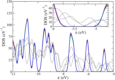
Figure 1: The density of states of a fullerene dimer calculated using a deterministic DFT approach (black curve), efsDFT with $I=80$ (red curve), $I=160$ (green curve) and $I=320$ (blue curve) stochastic orbitals. The dashed curves are sDFT results with $I=320$ stochastic orbitals for three different initial seeds. Inset: zoom into the energetic region of the gap.

We tested two generic cases for efsDFT and compared the results with sDFT and with a deterministic DFT approach (free of statistical errors), labeled dDFT below. The first test case involves a fullerene dimer with center-to-center separation of $\approx 1\mbox{nm}$ (the equilibrium value of bulk fullerene) as shown in Fig. 1. At this separation, the perturbation in the charge density of each fullerene caused by the neighboring monomer is rather small. Results based on sDFT using $I=320$ stochastic orbitals are shown for three different seeds (dashed curves). We find significant deviations of the density of states (DOS), caused by fictitious charge transfer between the monomers, and equally striking is the spread of the results. The charge sloshing phenomenon appears because of stochastic fluctuations, which in the case of weak coupling between the fragments leads to a spurious finite density of states inside the HOMO-LUMO gap. Increasing the number of stochastic orbitals will eventually fix this problem but at a much higher numerical cost. In fact, the number of stochastic orbitals required to converge the results in sDFT increases for weaker coupling between the fragments.

Figure 2: The density of states near the highest occupied and lowest unoccupied KS eigenvalues of $\left(H_{2}O\right)_{41}$ (left panel) and $\left(H_{2}O\right)_{191}$ (right panel) using sDFT with $I=320$ (cyan) and efsDFT with $I=80$ (red), $160$ (green) and $320$ (magenta) stochastic orbitals. The solid black curve represents the deterministic DFT calculation.

Table 1: efsDFT (and in one case sDFT) based results and corresponding deterministic values (dDFT) for the three systems studied for different number of random orbitals $I$. The following energies (in eV) are considered: HOMO ($\varepsilon_{HOMO}$) and LUMO ($\varepsilon_{LUMO}$) , total energy $E_{tot}$ and total energy per electron $E_{tot}/N_{e}$. The numbers in parenthesis are the standard deviation in the last given digit(s) estimated from 5 independent runs.

System	Method	$I$	$\varepsilon_{HOMO}$	$\varepsilon_{LUMO}$	$E_{tot}$	$E_{tot}/N_{e}$
$\left(\mbox{$H_{2}$O}\right)_{41}$	efsDFT	$80$	$-5.8\left(3\right)$	$-2.5\,\left(2\right)$	$-19129\,\left(1\right)$	$-58.320\,\left(4\right)$
		$160$	$-6.1\,\left(1\right)$	$-2.3\,\left(1\right)$	$-19128\,\left(1\right)$	$-58.317\,\left(4\right)$
		$320$	$-6.1\,\left(1\right)$	$-2.3\,\left(1\right)$	$-19126.9\,\left(7\right)$	$-58.314\,\left(2\right)$
	dDFT		$-5.9$	$-2.4$	$-19127.0$	$-58.314$
$\left(\mbox{$H_{2}$O}\right)_{191}$	efsDFT	$80$	$-5.0\,\left(3\right)$	$-2.60\,\left(5\right)$	$-89212\,\left(3\right)$	$-58.385\,\left(2\right)$
		$160$	$-5.5\,\left(2\right)$	$-2.66\,\left(7\right)$	$-89210\,\left(1\right)$	$-58.384\,\left(1\right)$
		$320$	$-5.7\,\left(1\right)$	$-2.55\,\left(6\right)$	$-89209\,\left(1\right)$	$-58.383\,\left(1\right)$
	dDFT		$-5.6$	$-2.48$	$-89208$	$-58.382$
$C_{60}$-$C_{60}$	sDFT	$320$	$-5.559\,\left(130\right)$	$-4.889(122)$	$-18701.0\,\left(30\right)$	$-38.9610\,\left(60\right)$
	efsDFT	$80$	$-5.925\,\left(25\right)$	$-4.823\,\left(29\right)$	$-18713.3\,\left(5\right)$	$-38.9861\,\left(10\right)$
		$160$	$-5.964\,\left(9\right)$	$-4.755\,\left(21\right)$	$-18713.1\,\left(3\right)$	$-38.9857\,\left(6\right)$
		$320$	$-5.969\,\left(2\right)$	$-4.752\,\left(4\right)$	$-18713.3\,\left(2\right)$	$-38.9861\,\left(4\right)$
	dDFT		$-5.973$	$-4.746$	$-18713.1$	$-38.9857$

Using the efsDFT with deterministic KS orbitals taken from each of the monomers yields a very rapid convergence of the DOS with the number of stochastic orbitals, as shown in Fig. 1 (red, green and blue curves). Importantly, a clear HOMO-LUMO gap is observed even when we use a very small number of stochastic orbitals. Furthermore, we do not observe the aforementioned spurious charge transfer between the two monomers.

The second test case involves two water clusters, with $41$ and $191$ molecules. The purpose is (1) to study a system with short-range order and long-range disorder and (2) to explore the efsDFT computational scaling with system-size. We used molecular dynamics (MD) with the flexible SPC forces field and a smooth cutoff Fennell and Gezelter (2006) to generate the disordered structures. The last time step configuration of the equilibrated trajectory was taken as the input structure for the efsDFT, sDFT and dDFT calculations.

In Fig. 2 we compare the efsDFT and dDFT calculations for the two water clusters. The sDFT calculations, which are shown only for the smaller cluster with $I=320$, preserve a gap in the density of states near the Fermi energy. However, due to unrealistic charge fluctuations there is a pronounced shift in the Fermi energy and a significant deformation of the DOS. In contrast, the efsDFT calculations, which used individual water molecules as the fragments, displays quantitative DOS already for $I=160$.

In Table 1 we summarize the results for the HOMO and LUMO orbital energies, and the total energy and total energy per electron. For the fullerene dimer, at $I=320$, sDFT deviates from the deterministic approach by $\approx 400\mbox{meV}$ and $\approx 150\mbox{meV}$ for the HOMO and LUMO orbital energies, respectively, while efsDFT is accurate to within a few meV’s. Moreover, the total energy per electron in sDFT deviates significantly from the deterministic value while efsDFT provides an accurate estimate to within a fraction of an meV.

A similar picture emerges for the water clusters. For example, the statistical error and the deviation from the deterministic approach in the HOMO and LUMO orbital energies are $50-100\,\mbox{meV}$ using $I=320$ for the larger water cluster. Further, the statistical error and deviation from deterministic values of the orbital and per-electron energies decrease with cluster size for a fixed number of stochastic orbitals, indicating self-averaging.Baer, Neuhauser, and Rabani (2013) Since the scaling of the approach with system size is linear for a fixed number of stochastic orbitals, this self-averaging suggests that for a given statistical error the new approach scales sub-linearly, similar to sDFT for homogeneous covalent systems.

In summary, we presented a new DFT method which combines features from both embedded and stochastic density functional theories. The densities of small fragments of the system were calculated by a deterministic DFT approach and were used to reconstruct the total density of the system deploying stochastic orbitals in a trace formula. The resulting method, so called efsDFT, preserves the scaling of sDFT, including the concept of self-averaging. Moreover, it overcomes some the limitations of sDFT, specifically for weakly coupled systems, achieving much faster convergence with the number of stochastic orbitals for both the density of states as well as for the total energy of the system. This was shown for two generic models, a weakly bound fullerene dimer and disordered clusters of water molecules.

efsDFT could be improved by a more sophisticated choice of the fragments, i.e., one that minimizes the density difference $\left|n\left(\mathbf{r}\right)-n_{F}\left(\mathbf{r}\right)\right|$. For example, one could self consistently improve the fragment Hamiltonians during the SCF iterations or “carve” them out of the total potential if easier. Even overlapping fragments could be used. This is because Eq. 5 is exact regardless of the choice of $n_{F}\left(\mathbf{r}\right)$. Work along these lines and others is currently in progress.

R. B. and E. R. gratefully thank the Israel Science Foundation, Grants No. 1020/10 and No. 611/11, respectively. R. B. and D. N. acknowledge the support of the US-Israel Bi-National Science Foundation. D. N. gratefully acknowledges support by the NSF, grant CHE-1112500.

References

- Hohenberg and Kohn (1964) P. Hohenberg and W. Kohn, Phys. Rev. 136, B864 (1964).
- Kohn and Sham (1965) W. Kohn and L. J. Sham, Phys. Rev. 140, A1133 (1965).
- Kolb and Thonhauser (2012) B. Kolb and T. Thonhauser, Nano LIFE 2 (2012).
- Chelikowsky et al. (2011) J. R. Chelikowsky, M. Alemany, T. Chan, and G. Dalpian, Rep. Prog. Phys. 74, 046501 (2011).
- Frauenheim et al. (2002) T. Frauenheim, G. Seifert, M. Elstner, T. Niehaus, C. Kohler, M. Amkreutz, M. Sternberg, Z. Hajnal, A. Di Carlo, and S. Suhai, J. Phys.: Conden. Mat. 14, 3015 (2002).
- Baroni et al. (2001) S. Baroni, S. de Gironcoli, A. Dal Corso, and P. Giannozzi, Rev. Mod. Phys. 73, 515 (2001).
- Siegbahn and Himo (2009) P. E. Siegbahn and F. Himo, J. Bio. Inorg. Chem. 14, 643 (2009).
- Schwegler and Challacombe (1996) E. Schwegler and M. Challacombe, J. Chem. Phys. 105, 2726 (1996).
- Baer and Head-Gordon (1997) R. Baer and M. Head-Gordon, Phys. Rev. Lett. 79, 3962 (1997).
- Goedecker (1999) S. Goedecker, Rev. Mod. Phys. 71, 1085 (1999).
- Scuseria (1999) G. E. Scuseria, J. Phys. Chem. A 103, 4782 (1999).
- Soler et al. (2002) J. M. Soler, E. Artacho, J. D. Gale, A. Garcia, J. Junquera, P. Ordejon, and D. Sanchez-Portal, J. Phys. C 14, 2745 (2002).
- Skylaris et al. (2005) C. K. Skylaris, P. D. Haynes, A. A. Mostofi, and M. C. Payne, J. Phys. C 17, 5757 (2005).
- Gillan et al. (2007) M. J. Gillan, D. R. Bowler, A. S. Torralba, and T. Miyazaki, Comput. Phys. Commun. 177, 14 (2007).
- Zeller (2008) R. Zeller, J. Phys.: Conden. Mat. 20, 294215 (2008).
- Wang, Zhao, and Meza (2008) L.-W. Wang, Z. Zhao, and J. Meza, Phys. Rev. B , 165113 (2008).
- Ozaki (2010) T. Ozaki, Phys. Rev. B 82, 075131 (2010).
- Rudberg, Rubensson, and Salek (2010) E. Rudberg, E. H. Rubensson, and P. Salek, J. Chem. Theor. and Comput. 7, 340 (2010).
- Baer, Neuhauser, and Rabani (2013) R. Baer, D. Neuhauser, and E. Rabani, Phys. Rev. Lett. 111, 106402 (2013).
- Daw and Baskes (1984) M. S. Daw and M. I. Baskes, Physical Review B 29, 6443 (1984).
- Wesolowski and Warshel (1993) T. A. Wesolowski and A. Warshel, J. Phys. Chem. 97, 8050 (1993).
- Svensson et al. (1996) M. Svensson, S. Humbel, R. D. Froese, T. Matsubara, S. Sieber, and K. Morokuma, J. Phys. Chem. 100, 19357 (1996).
- Govind, Wang, and Carter (1999) N. Govind, Y. A. Wang, and E. A. Carter, The Journal of chemical physics 110, 7677 (1999).
- Lin and Truhlar (2007) H. Lin and D. G. Truhlar, Theor. Chem. Acc. 117, 185 (2007).
- Elliott et al. (2010) P. Elliott, K. Burke, M. H. Cohen, and A. Wasserman, Phys. Rev. A 82 (2010).
- Goodpaster et al. (2010) J. D. Goodpaster, N. Ananth, F. R. Manby, and T. F. Miller III, J. Chem. Phys. 133, 084103 (2010).
- Kosloff (1988) R. Kosloff, J. Phys. Chem. 92, 2087 (1988).
- Rom, Charutz, and Neuhauser (1997) N. Rom, D. Charutz, and D. Neuhauser, Chemical physics letters 270, 382 (1997).
- Pulay (1980) P. Pulay, Chem. Phys. Lett. 73, 393 (1980).
- Fennell and Gezelter (2006) C. J. Fennell and J. D. Gezelter, The Journal of chemical physics 124, 234104 (2006).