An R Implementation of the Pólya-Aeppli Distribution

Abstract

An efficient implementation of the Pólya-Aeppli, or geometirc compound Poisson, distribution in the statistical programming language R is presented. The implementation is available as the package polyaAeppli and consists of functions for the mass function, cumulative distribution function, quantile function and random variate generation with those parameters conventionally provided for standard univatiate probability distributions in the stats package in R

1 Introduction

A Pólya-Aeppli or geometric compound Poisson random variable is defined as the sum of a Poisson number of independent and identically distributed geometric random variables [8, 4]. Its distribution arises as an approximation to the distribution of the number of occurrences of a given short word in a random Markovian sequence of letters from a finite alphabet [10, 9], and as an approximation to the number of word matches between two random sequences [5]. Thus the Polya-Aeppli distribution finds applications in bioinformatics in searches for over- or underrepresented words, which may signal functional elements within genomes, and applications associated with alignment-free measures of sequence similarity. It is also appropriate as an alternative to the commonly used negative binomial model of over-dispersed Poisson count data which arises, for instance, from high throughput sequencing experiments [2].

The stats package in R [11] contains implementations of many standard univariate probability distributions as functions for the density/mass function, cumulative distribution function, quantile function and random variate generation. We present here an efficient implementation of these 4 functions for the Pólya-Aeppli distribution, available as the package polyaAeppli [1]. The implementation relies on iterative formulae for the log of the mass and cumulative distribution functions, which allow an accurate evaluation of the distribution in the extreme upper and lower tails.

We define a Pólya-Aeppli random variable as

$$X=\sum_{i=1}^{N}Y_{i}$$ (1)

where $N$ is a Poisson random variable with parameter $\lambda$ with probability mass function

$$P_{N}(n;\lambda)=\mbox{$\rm{Prob}$\,}(N=n)=\frac{e^{-\lambda}\lambda^{n}}{n!},\qquad n=0,1,\ldots,$$ (2)

and the $Y_{i}$ are identically and independently distributed shifted geometric random variables with parameter $p$ with common probability mass function

$$P_{Y}(y;p)=\mbox{$\rm{Prob}$\,}(Y=y)=p^{y-1}(1-p),\qquad y=1,2,\ldots.$$ (3)

The Pólya-Aeppli probability mass function is [4]

$$P_{X}(x;\lambda,p) = \mbox{$\rm{Prob}$\,}(X=x)$$ (4)

$$= \begin{cases}e^{-\lambda}&\mbox{if $x=0$}\\ e^{-\lambda}\displaystyle\sum_{n=1}^{y}\frac{\lambda^{n}}{n!}{{y-1}\choose{n-1}}p^{y-n}(1-p)^{n}&\mbox{if $x=1,2,\ldots$.}\end{cases}$$

The mean and variance are

$$E(X)=\mu=\frac{\lambda}{1-p},\quad\mbox{$\rm{Var}$\,}(X)=\sigma^{2}=\lambda\frac{1+p}{(1-p)^{2}}.$$ (5)

These formulae invert to give

$$\lambda=\frac{2\mu^{2}}{\sigma^{2}+\mu},\quad p=\frac{\sigma^{2}-\mu}{\sigma^{2}+\mu}.$$ (6)

Note that the restriction $0\leq p<1$ implies that $\sigma^{2}>\mu$, making ths distribution a suitable model for over-dispersed count data. When $p=0$, the Póya-Aeppli distribution reduces to the Poisson distribution with mean $\lambda$.

2 Implementation

Consistent with the conventions used in R, our implementation comprises the four functions

dPolyaAeppli(x, lambda, prob, log = FALSE)
pPolyaAeppli(q, lambda, prob, lower.tail = TRUE, log.p = FALSE)
qPolyaAeppli(p, lambda, prob, lower.tail = TRUE, log.p = FALSE)
rPolyaAeppli(n, lambda, prob)

for the mass function, cumulative distribution function, quantile function and random variate generation respectively. The arguments lambda and prob accept single values for the parameters $\lambda$ and $p$ respectively. The argument x is a vector of (non-negative integer) quantiles, q is a vector of quantiles, p is a vector of probabilities and n is the number of random values to return. If the logical variables log or log.p are TRUE, probabilities are given as logarithms to base $e$. If the logical variable lower.tail is set to its default value of TRUE probabilities are $\mbox{$\rm{Prob}$\,}(X\leq x)$, otherwise probabilities are $\mbox{$\rm{Prob}$\,}(X>x)$. Examples of plots of the cumulative distribution, mass function and a histogram of a random sample are shown in Figure 1 for values of $\lambda$ and $p$ corresponding to a mean $\mu=10$ and variance $\sigma^{2}=15$.

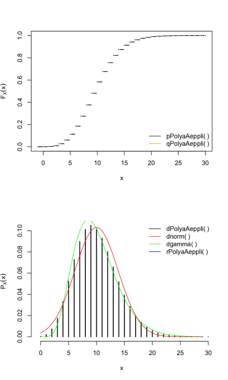
Figure 1: The Pólya-Aeppli distribution for values of $\lambda$ and $p$ corresponding to mean $\mu=10$ and variance $\sigma^{2}=15$. Top panel: the cumulative distribution calculated from pPolyaAeppli() (black) and quantiles calculated from qPolyaAeppli() plotted on the horizontal axis against probabilites in the range $[0,1)$ plotted on the vertical axis (orange). Bottom panel: The probability mass function calculated from dPolyaAeppli() (black) and a histogram of 10 000 random variables sampled using rPolyaAeppli(). Also plotted for comparison are normal (red) and gamma (green) distributions with matching mean and variance.

The option log = TRUE allows for a more precise determination of the distribution in the extreme tails when dPolyaAeppli() would otherwise return 0 to machine accuracy. The option log.p = TRUE allows for an accurate determination of the cumulative distribution using pPolyaAeppli() and its inverse using qPolyaAeppli() in the extreme lower and upper tails when used in conjunction with lower.tail = TRUE and FALSE respectively. Plots of the mass function and cumulative distribution over a range of quantiles more than 60 standard deviations either side of the mean for values of $\lambda$ and $p$ corresponding to mean $\mu=4000$ and variance $\sigma^{2}=4050$ are shown in Figure 2.

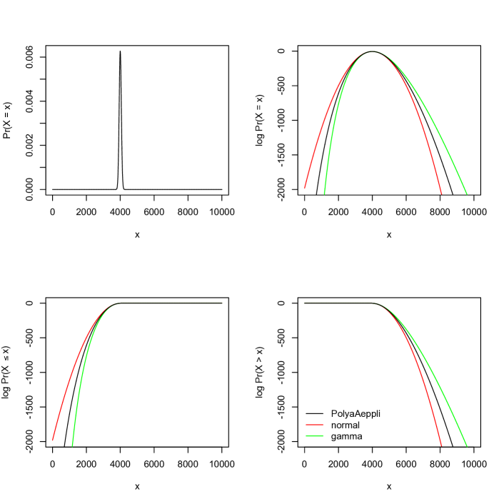
Figure 2: Extreme tails of the Pólya-Aeppli distribution for values of $\lambda$ and $p$ corresponding to mean $\mu=4000$ and variance $\sigma^{2}=4050$. Top left: The mass function calculated using dPolyaAeppli() with defaults. Top right: Log of the mass function using dPolyaAeppli(…, log=TRUE). Bottom left: Log of the lower tail of the cumulative distribution calculated using pPolyaAeppli(…, log.p=TRUE). Bottom right: Log of the upper tail of the cumulative distribution calculated using pPolyaAeppli(…, log.p=TRUE, lower.tail = FALSE). Also plotted for comparison are normal (red) and gamma (green) distributions with equivalent parameters.

R implementations of the Pólya-Aeppli mass function and random variate generator, but not the cumulative distribution function or quantile function, currently exist via the Poisson-Tweedie distribution in the package tweeDEseq [2]. The function dPT(x, mu = lambda/(1 - prob), D = (1 + p)/(1 - p), a = -1) plays the role of dPolyaAeppli(x, lambda, prob), and the function
rPT(n, mu = lambda/(1 - prob), D = (1 + p)/(1 - p), a = -1) plays the role of rPolyaAeppli(n, lambda, prob). However, because the log = TRUE option is not implemented, dPT() is not able to evaluate the distribution as accurately as dPolyaAeppli(…, log = TRUE) in the extreme tails of the distribution. Furthermore the tweeDEseq implementations are not vectorised over the parameters of the distribution.

An R implementation of the upper tail of the Pólya-Aeppli distribution was previously implemented via the now discontiued function computePValue() in the package NeMo [7] for the study of network motifs. This function, with arguments computePValue(lambda, prob, 1+x) played the same role as pPloyaAeppli(x, lambda, prob, lower.tail=FALSE), but was not vectorised over either the argument x or the parameters lambda or prob. Furthermore the option log.p=TRUE, was not implemented, making the extreme tails of the distribution inaccessible.

3 Algorithms

The implementation of the Pólya-Aeppli distribution must be able to evaluate the mass function and cumulative distribution function efficiently for a range of input quantiles. From Eq. (4) Evens [3] has derived the recurrence formula

$$(x+1)P_{X}(x+1;n,\lambda)=$$ (7)

$$[\lambda(1-p)+2px]P_{X}(x;n,\lambda)-p^{2}(x-1)P_{X}(x-1;n,\lambda),\quad x=1,2,\ldots,$$

with

$$P_{X}(0;n,\lambda)=e^{-\lambda},\quad P_{X}(1;n,\lambda)=\lambda(1-p)e^{-\lambda}.$$ (8)

As is stands this formula is not adequate for our purposes as it susceptible to roundoff errors when $e^{-\lambda}$ is small, which may happen for instance when $\mu$ is moderately large and $\sigma^{2}/\mu$ close to 1. Nuel [6] notes that this problem is overcome by calculating instead the logarithm of the mass function

$$l(x)=\log P_{X}(x;n,\lambda),$$ (9)

from the recurrence relation

$$l(x+1)=\log\left\{\frac{\lambda(1-p)+2px-p^{2}(x-1)e^{l(x-1)-l(x)}}{x+1}\right\}+l(x),\quad x=1,2,\ldots,$$ (10)

$$l(0)=-\lambda,\quad l(1)=-\lambda+log\lambda(1-p),$$ (11)

which is easily derived from Eq.(7). The function dPolyaAeppli(x, lambda, prob) is calculated by first evaluating this iterative formula out to the largest finite value in the array x and exponentiating if log=FALSE.

To calculate the lower tail of cumulative distribution

$$F_{X}(x)=\mbox{$\rm{Prob}$\,}(X\leq x)=\sum_{i=0}^{\lfloor x\rfloor}P_{X}(i),\quad x\in\mathds{R},$$ (12)

Nuel [6] similarly avoids serious roundoff errors by calculating the logarithm of the cumulative distribution function

$$g(x)=\log F_{X}(x),$$ (13)

from the recurrence relation

$$g(i+1)=g(i)+\log\left(1+e^{l(i+1)-g(i)}\right),\quad i=0,1,2,\ldots$$ (14)

$$g(0)=\lambda.$$ (15)

The function pPolyaAeppli(x, lambda, prob, lower.tail = TRUE) is calculated by first evaluating Eqs. (10) and (14) out to the integer part of the largest finite value in the array x and exponentiating if necessary.

This procedure will not meet the required accuracy for the extreme upper tail. In this case we consider the log of the upper tail,

$$h(x)=\log(1-F_{X}(x))=\log\mbox{$\rm{Prob}$\,}(X>x),$$ (16)

which can be iterated downwards via the formula

$$h(i-1)=h(i)+\log(1+e^{l(i)-h(i)}),\quad i=\lfloor x_{\rm max}\rfloor,\lfloor x_{\rm max}\rfloor-1,\lfloor x_{\rm max}\rfloor-2,\ldots,1.$$ (17)

To evaluate pPolyaAeppli(x, lambda, prob, lower.tail = FALSE) where x includes finite values greater than the mean $\mu$, $x_{\rm max}$ is taken to be the largest finite value in the array x, and Eq.(17) is initiated by calculating

$$h(\lfloor x_{\rm max}\rfloor)=l(\lfloor x_{\rm max}\rfloor+1)+\log\sum_{i=\lfloor x_{\rm max}\rfloor+1}^{\infty}e^{l(i)-l(\lfloor x_{\rm max}\rfloor+1)},$$ (18)

which converges to machine accuracy reasonably rapidly.

The functions $l(x)$, $g(x)$ and $h(x)$ are calculated by auxilliary functions
lPolyaAeppliArray(), gArray() and hArray(), and $h(x_{\rm max})$ is evaluated by the auxilliary function logTail().

The quantile function qPolyaAeppli() is evaluated by first evaluating probabilities with pPolyaAeppli() from q $=0$ out to a safe upper bound, and seeking the maximum q entailing a probability less than the specified probability for each value in the input array p. The upper bound used is the value of he quantile function qgamma() of the gamma distribution with matching mean and variance (see Fig. 2) evaluated at the maximum finite value in the input array p, plus one standard deviation.

The function rPolyaAeppli() is evaluated directly from the definition Eq.(1) via the R functions rpois() and rgeom().

References

- [1] C.J. Burden. polyaAeppli: Implementation of the Pólya-Aeppli distribution. R cran package version 2.0, 2014.
- [2] Mikel Esnaola, Pedro Puig, David Gonzalez, Robert Castelo, and Juan R Gonzalez. A flexible count data model to fit the wide diversity of expression profiles arising from extensively replicated rna-seq experiments. BMC Bioinformatics, 14:254, 2013.
- [3] D.A. Evans. Experimental evidence concerning contagious distributions in ecology. Biometrika, 40:186–211, 1953.
- [4] N. L. Johnson, S. Kotz, and A. W. Kemp. Univariate Discrete Distributions. Wiley, New York, 2nd edition, 1992.
- [5] R. A. Lippert, H. Huang, and M. S. Waterman. Distributional regimes for the number of -word matches between two random sequences. Proc. Natl. Acad. Sci. USA, 99(22):13980–9, 2002.
- [6] G. Nuel. Cumulative distribution function of a geometeric poisson distribution. Journal of Statistical Computation and Simulation, 78(3):385–394, 2008.
- [7] F. Picard, J.J. Daudin, M. Koskas, S. Schbath, and S. Robin. Assessing the exceptionality of network motifs. Journal of Computational Biology, 15:1–20, 2008.
- [8] G. Pólya. Sur quelques points de la théorie des probabilitiés. Annales de l’Instut H. Poincaré, 1:117–161, 1930.
- [9] S. Robin and S. Schbath. Numerical comparison of several approximations of the word count distributions in random sequences. Journal of Computational Biology, 8(4):349–359, 2001.
- [10] S. Schbath. Compound poisson approximation of word counts in DNA sequences. ESIAM: Probability and Statistics, 1:1–16, 1995.
- [11] R Development Core Team. R: A language and environment for statistical computing, 2001.