Learning with Cross-Kernels and Ideal PCA

Abstract

We describe how cross-kernel matrices, that is, kernel matrices between the data and a custom chosen set of ‘feature spanning points’ can be used for learning. The main potential of cross-kernels lies in the fact that (a) only one side of the matrix scales with the number of data points, and (b) cross-kernels, as opposed to the usual kernel matrices, can be used to certify for the data manifold. Our theoretical framework, which is based on a duality involving the feature space and vanishing ideals, indicates that cross-kernels have the potential to be used for any kind of kernel learning. We present a novel algorithm, Ideal PCA (IPCA), which cross-kernelizes PCA. We demonstrate on real and synthetic data that IPCA allows to (a) obtain PCA-like features faster and (b) to extract novel and empirically validated features certifying for the data manifold.

1.  Introduction

Since their invention by Boser, Guyon and Vapnik [2, 7], kernel methods have had a fundamental impact on the fields of statistics and machine learning. The major appeal of using kernel methods for learning consists in using the kernel trick, first proposed by Aizerman, Braverman and Rozonoer [1], which allows to make otherwise costly computations in the feature space implicit and thus highly efficient for a huge variety of learning tasks – see e.g. [4, 6] for an overview.

Many kernel methods make extensive use of the so-called kernel matrix, a matrix whose entries are kernel function evaluations $k(x_{i},x_{j})$ at data points $x_{1},\dots,x_{N}\in\mathbb{R}^{n}$. This kernel matrix $K_{\!X\!X}=(k(x_{i},x_{j}))_{ij}$ is simultaneously the main source of efficient linearization and the central computational bottleneck. For instance, the most expensive part of algorithms such as kernel PCA or kernel ridge regression consists in computing the inverse or a singular value decomposition of the $(N\times N)$ matrix $K_{\!X\!X}$. We make two observations in this context:

(A) Subsampling $K_{\!X\!X}$, i.e., considering $(N\times M)$ sub-matrices of $K_{\!X\!X}$, is the state-of-the-art in speeding up the scalability in the number of data points $N$. While much has been written on the topic, there seems to be no consensus on how exactly to choose the subsample from the data set.

(B) There seems to be no kernel algorithm which learns the data manifold from which the $x_{i}$ were obtained, or test whether an unseen data point is on the manifold - in particular none involving $K_{\!X\!X}$. (Note that kernel PCA outputs projections on predominant data coordinates, but not the coordinates embedded in data space or the shape of the data manifold.)

In this paper, we propose an algebraic duality framework which offers both a potential explanation and a potential solution to the above (seemingly unrelated) issues. Our contribution is centered around cross-kernel matrices $K_{\!X\!Z}=(k(x_{i},z_{j}))_{ij}$, where $z_{1},\dots,z_{M}\in\mathbb{R}^{n}$, called cross-kernel basis points, are not necessarily data points. Assuming that $z_{1},\dots,z_{M}$ are chosen suitably (e.g., randomly) and that $M$ is large enough, we show theoretically and empirically that:

(1) The cross-kernel matrix $K_{\!X\!Z}$ can be used to capture both the information contained in $K_{\!X\!X}$ as well as additional information about the data manifold which is provably not contained in $K_{\!X\!X}$. Practically, we present an algorithm, called IPCA, which is able to learn both coordinates in the manifold as well as certificates for being contained in the data manifold, addressing issue (B) above.

(2) The cross-kernel matrix $K_{\!X\!Z}$ can be employed in ways completely analogous to a subsampled matrix $K_{\!X\!X}$. As opposed to subsampling, the properties of the points $z_{i}$ can be prescribed by the experimenter and are thus independent of known or unknown – and potentially detrimental – properties of the data $x_{i}$. In particular, $K_{\!X\!Z}$ can be used for speeding up kernel learning, while potentially avoiding data-related subsampling issues, thereby addressing issue (A) above.

In the following we briefly explain why and how considering the cross-kernel $K_{\!X\!Z}$ can be advantageous as compared to the kernel matrix $K_{\!X\!X}$. More detailed technical statements and explicit algorithms can be found in section 2 and thereafter.

Why the kernel matrix is not enough. The kernel matrix $K_{\!X\!X}$ misses information on the data manifold that can be obtained from $K_{\!X\!Z}$. Let us explain this in the example where the kernel is the ordinary Euclidean scalar product $k(x,y)=\langle x,y\rangle$ in $\mathbb{R}^{n}$. Suppose the data points $x_{1},\dots,x_{N}$ all lie in a vector subspace $L\subseteq\mathbb{R}^{n}$. The entries of the kernel matrix $K_{\!X\!X}$ are scalar products of the type $\langle x_{i},x_{j}\rangle$ which are invariant under rotation of the coordinate system. Therefore, one obtains one and the same kernel matrix $K_{\!X\!X}$ when considering rotated data points $Ux_{1},\dots,Ux_{N}$ and the rotated vector space $U\cdot L$ for any rotation matrix $U\in\mathbb{R}^{n\times n}$. Since one and the same kernel matrix $K_{\!X\!X}$ can arise in a non-degenerate way from every vector space $L$ (of that dimension), the data manifold $L$ can not be obtained back from $K_{\!X\!X}$. Similar considerations hold for arbitrary kernels: the data manifold can not be learnt from the kernel matrix $K_{\!X\!X}$.

Cross-kernels help! In the above example the vector space $L$ can be identified from a cross-kernel matrix $K_{\!X\!Z}=(k(x_{i},z_{j}))_{ij}$, if $z_{1},\dots,z_{M}$ span $\mathbb{R}^{n}$. Observe that the rows of $K_{\!X\!Z}$ are coordinate representations of the $x_{i}$. Since $z_{1},\dots,z_{M}$ span $\mathbb{R}^{n}$, the data point $x_{i}$ can be obtained back from the $i$-th row of $K_{\!X\!Z}$. Since reconstructing $x_{i}$ from the $i$-th row of $K_{\!X\!Z}$ is a linear reparameterization, an unseen data point $x$ is contained in the data manifold $L$ if and only if the vector $\kappa_{z}(x)=(k(x,z_{j}))_{j}$ is contained in the row-span of $K_{\!X\!Z}$. Therefore we can obtain $L$ back from $K_{\!X\!Z}$ and use the row-span of $K_{\!X\!Z}$ to efficiently test membership for the data manifold $L$. Note that the same reasoning does not work for the matrix $K_{\!X\!X}$, since $x_{1},\dots,x_{N}$ do not span $\mathbb{R}^{n}$, but only $L$. A similar reasoning holds in larger generality: the cross-kernel $K_{\!X\!Z}$ contains extensive information on the data manifold which $K_{\!X\!X}$ does not.

From cross-kernels to kernel learning. The “manifold awareness” of the cross-kernel implies further interesting properties which can be used for decomposing, and thus approximating, the original kernel matrix $K_{\!X\!X}$ via the potentially much smaller $K_{\!X\!Z}$. Namely, letting $K_{\!Z\!X}=K_{\!X\!Z}^{\top}$ and $K_{\!Z\!Z}=(k(z_{i},z_{j}))_{ij}$, we can show that the equality $K_{\!X\!X}=K_{\!X\!Z}K_{\!Z\!Z}^{-1}K_{\!Z\!X}$ holds exactly for polynomial kernels (assuming “feature-spanning” points $z_{i}$ as in the example above, see Theorem 3.4). We conjecture (and have observed empirically) that the same holds approximately for other kernels. This equality is reminiscent of the central equation in subsampling, with the difference that the points $z_{j}$ do not need to be chosen among the data. Suitable choices of the points $z_{j}$ avoid potential problems in the data while leading to the same speed-up of arbitrary kernel methods.

2.  Some dualities for polynomial kernels

The following preview of our approach is a more technically exact and quantitative variant of the discussion in the introduction. In what follows, we use inhomogenous polynomial kernels. (A further difficulty, not considered here, lies in the generalization to other kernels and kernel feature spaces.) The central observation which we to carry over from the introduction is the certifying property of the row-span of $K_{\!X\!Z}$. In our setup, the data points $x_{i}$ are sampled from a manifold $\mathcal{X}\subset\mathbb{R}^{n}$ which is “cut out” by an unknown set of polynomial equations. Our goal is to relate these equations to the linear span of the images $\Phi_{\leq d}(x_{i})$ under the feature map $\Phi_{\leq d}$. This linear span is then related to the row-span of $K_{\!X\!Z}$ by applying several dualities in and on feature space.

More technically, we first show how to identify $\mathbb{R}[\mathbf{t}]_{\leq d}$, the set of polynomials of degree at most $d$, with linear functionals on the kernel feature space and that every $f\in\mathbb{R}[\mathbf{t}]_{\leq d}$ can be expressed as a kernel decision function. To understand the equations cutting out $\mathcal{X}$ (which are not canonical) it is better to change perspective and consider the set of all polynomials vanishing on $\mathcal{X}$, called its vanishing ideal (which is canonical). The main results of this section say, informally, that $\mathcal{X}$ can be identified with the intersection of a particular linear space $L$ and $\Phi_{\leq d}(\mathbb{R}^{n})$, and that the vanishing ideal of $\mathcal{X}$ corresponds to $L^{\perp}$, which in turn is isomorphic to the row-span of $K_{\!X\!Z}$. In other words, we relate a linear duality to the algebraic-geometric concept of duality between sets of equations and their common vanishing locus.

2.1.  Duality of polynomial rings and feature spaces

To begin with, we introduce inhomogeneous polynomial kernel as follows.

Definition 2.1.

Let $\theta\in(0,1)$ be a fixed real number, and let $d\geq 1$. The inhomogeneous polynomial kernel function $k_{\leq d}:\;\mathbb{R}^{n}\times\mathbb{R}^{n}\longrightarrow\mathbb{R}$ is given by $k_{\leq d}(x,y)=(\theta\cdot\langle x,y\rangle+1)^{d}$, where $\langle.,.\rangle$ denotes the standard scalar product.

This definition differs slightly from the usual one which is obtained after dividing by $\theta^{d}$. Since $\theta$ is chosen arbitrarily in $(0,1)$, no qualitative change is introduced by our convention. It is however, as we will see, the more natural one.

It is well-known that feature space $\mathcal{F}_{\leq d}$ of $k_{\leq d}$ satisfies $\mathcal{F}_{\leq d}\cong\mathbb{R}^{m}$, where $m=\binom{n+d}{d}$, and that the feature map $\Phi_{\leq d}:\;\mathbb{R}^{n}\longrightarrow\mathcal{F}_{\leq d}$ is given by $\Phi_{\leq d}(x)=(\gamma_{\alpha}x^{\alpha}\mid|\alpha|\leq d)$ (e.g., see [4], Sec. 2.1). Here we let $x^{\alpha}=c_{1}^{\alpha_{1}}\cdots c_{n}^{\alpha_{n}}$ and $|\alpha|=\alpha_{1}+\cdots+\alpha_{n}$ for $x=(c_{1},\dots,c_{n})$ and $\alpha=(\alpha_{1},\dots,\alpha_{n})$. Moreover, we have $\gamma_{\alpha}=\sqrt{\theta^{|\alpha|}\cdot\binom{d}{|\alpha|}\cdot\binom{|\alpha|}{\alpha_{1},\dots,\alpha_{n}}}$. To define $\Phi_{\leq d}$ uniquely, we order $p_{1},\dots,p_{m}$ increasingly with respect to the degree-lexicographic term ordering. The feature map is characterized by the property that $k_{\leq d}(x,y)=\langle\Phi_{\leq d}(x),\Phi_{\leq d}(y)\rangle$ for $x,y\in\mathbb{R}^{d}$, i.e., by the fact that it transforms the kernel function to a standard scalar product on the feature space.

On the algebraic side, the main objects linked via duality are vector spaces of polynomials. Let $\mathbf{t}=(t_{1},\dots,t_{n})$ be a tuple of indeterminates, and let $\mathbb{R}[\mathbf{t}]$ be the polynomial ring in these indeterminates. For every $d\geq 0$, we denote by $\mathbb{R}[\mathbf{t}]_{\leq d}$ the vector space of all polynomials of degree at most $d$. Recall that the dimension of $\mathbb{R}[\mathbf{t}]_{\leq d}$ is $\binom{n+d}{d}$. The inhomogeneous polynomial kernel function can be extended to a pairing of polynomials as follows.

Notation 2.2.

Let $\theta\in(0,1)$ and $d\geq 1$. The inhomogeneous polynomial kernel on $\mathbb{R}[\mathbf{t}]$ is the map $\mathbf{k}_{\leq d}:\ \mathbb{R}[\mathbf{t}]^{n}\times\mathbb{R}[\mathbf{t}]^{n}\longrightarrow\mathbb{R}[\mathbf{t}]$ given by $\mathbf{k}_{\leq d}(F,G)=(\theta\cdot\langle F,G\rangle+1)^{d}$ where we define $\langle F,G\rangle=f_{1}g_{1}+\cdots+f_{n}g_{n}$ for $F=(f_{1},\dots,f_{n})$ and $G=(g_{1},\dots,g_{n})$.

The polynomials $\mathbf{k}_{\leq d}(x,\mathbf{t})\in\mathbb{R}[\mathbf{t}]$ can be used to generate $\mathbb{R}(\mathbf{t}]_{\leq d}$, as our next proposition shows. By the multinomial theorem, they can be expressed as $\mathbf{k}_{\leq d}(x,\mathbf{t})=(\theta\langle x,\mathbf{t}\rangle+1)^{d}=\sum_{|\alpha|\leq d}\gamma_{\alpha}^{2}x^{\alpha}t^{\alpha}$. Recall that points $x_{1},\dots,x_{m}\in\mathbb{R}^{n}$ are called generic for a property $\mathcal{P}$ if there exists a Zariski open subset of $U\subseteq(\mathbb{R}^{n})^{m}$ such that property $\mathcal{P}$ holds for all $(x_{1},\dots,x_{m})\in U$.

Proposition 2.3.

Let $d\geq 0$, let $m^{\prime}\geq\binom{n+d}{d}$, and let $x_{1},\dots,x_{m^{\prime}}\in\mathbb{R}^{n}$ be generic. Then we have $\mathbb{R}[\mathbf{t}]_{\leq d}=\langle\mathbf{k}_{\leq d}(x_{i},\mathbf{t})\mid 1\leq i\leq m^{\prime}\rangle$.

The next proposition says that $\mathbb{R}[\mathbf{t}]_{\leq d}$ is dual to the feature space $\mathcal{F}_{\leq d}$.

Proposition 2.4.

(a) For $d\geq 1$, the map $\varphi:\,\mathbb{R}[\mathbf{t}]_{\leq d}\longrightarrow(\mathcal{F}_{\leq d})^{\vee}\cong{\rm Hom}_{\mathbb{R}}(\mathbb{R}^{m},\mathbb{R})$ defined by $f=\sum_{|\alpha|\leq d}\,c_{\alpha}{\mathbf{t}}^{\alpha}\mapsto f^{\vee}$, where $f^{\vee}(e_{\alpha})=c_{\alpha}/\gamma_{\alpha}$, is an isomorphism of $\mathbb{R}$-vector spaces.
(b) For $d\geq 1$, the map $\psi:\,\mathbb{R}[\mathbf{t}]_{\leq d}\longrightarrow\mathcal{F}_{\leq d}$ defined by $f=\sum_{|\alpha|\leq d}\,c_{\alpha}{\mathbf{t}}^{\alpha}\mapsto\sum_{|\alpha|\leq d}(c_{\alpha}/\gamma_{\alpha})e_{\alpha}$ is an isomorphism of $\mathbb{R}$-vector spaces.

By dualizing the map $\varphi$ and using the canonical isomorphism between $\mathcal{F}_{\leq d}$ and its bidual, we obtain an isomorphism $\varphi^{\vee}:\,\mathcal{F}_{\leq d}\longrightarrow(\mathbb{R}[\mathbf{t}]_{\leq d})^{\vee}$ which maps $e_{\alpha}$ to the $\mathbb{R}$-linear map given by $t^{\beta}\mapsto\gamma_{\alpha}\,\delta_{\alpha\beta}$. Another consequence of the preceding proposition is that, if we pass to the union $\mathbb{R}[\mathbf{t}]=\bigcup_{d\geq 1}\mathbb{R}[\mathbf{t}]_{\leq d}$, we see that the polynomial ring contains the duals of all feature spaces $\mathcal{F}_{\leq d}$.

Finally, we interpret the isomorphism $\varphi$ in terms of kernel decision functions. Recall that the map $\mathop{\rm eval}\nolimits(f):\,\mathbb{R}^{n}\longrightarrow\mathbb{R}$ given by $x\mapsto f(x)$ is called the polynomial function associated to $f\in\mathbb{R}[\mathbf{t}]$ and that the polynomial function associated to $\mathbf{k}_{\leq d}(x,\mathbf{t})$ is called a kernel decision function. Let us denote the vector space of all kernel decision functions by $\mathop{\rm KDF}\nolimits_{\leq d}$.

Corollary 2.5.

The map $\Phi_{\leq d}^{\ast}:\,(\mathcal{F}_{\leq d})^{\vee}\longrightarrow\mathop{\rm KDF}\nolimits_{\leq d}$ given by $\ell\mapsto\ell\circ\Phi_{\leq d}$ is an isomorphism.

Now we use the isomorphism $\varphi:\ \mathbb{R}[\mathbf{t}]_{\leq d}\longrightarrow(\mathcal{F}_{\leq d})^{\vee}$ to transfer the standard scalar product on $\mathcal{F}_{\leq d}$ to $\mathbb{R}[\mathbf{t}]_{\leq d}$ in the natural way. The result is a scalar product $\langle.,.\rangle_{\varphi}$ on $\mathbb{R}[\mathbf{t}]_{\leq d}$ such that

$$\langle\mathbf{t}^{\alpha},\mathbf{t}^{\beta}\rangle_{\varphi}\;=\;\langle(1/\gamma_{\alpha})\,e_{\alpha}^{\vee},\,(1/\gamma_{\beta})\,e_{\beta}^{\vee}\rangle\;=\;(1/\gamma_{\alpha}^{2})\,\delta_{\alpha\beta}$$

for $|\alpha|\leq d$. The next proposition provides a basic property of the scalar product $\langle.,.\rangle_{\varphi}$.

Proposition 2.6.

For $f\in\mathbb{R}[\mathbf{t}]_{\leq d}$ and $x\in\mathbb{R}^{n}$, we have $f(x)=\langle f,\mathbf{k}_{\leq d}(x,\mathbf{t})\rangle_{\varphi}$.

The duality expressed by the map $\varphi$ is an algebraic analogue of the theory of reproducing kernel Hilbert spaces. The associated Hilbert space is the space of polynomial functions $f:\mathbb{R}^{n}\rightarrow\mathbb{R}$ of degree $\leq d$ which can be identified with $\mathbb{R}[\mathbf{t}]_{\leq d}$ by replacing the polynomial function $f$ with the corresponding symbolic polynomial. The equation in the preceding proposition could also be obtained by combining the Riesz representation with this identification (see [4], Sec. 2.2). In the next section we go beyond what can be shown using the usual RKHS duality alone.

2.2.  Duality of vanishing ideals and feature spans

Next we show that ideals – a classical concept in algebra – are the proper dual objects of feature spans of manifolds, in the same way as the polynomial ring is the dual of feature space itself. Recall that an ideal $I$ in $\mathbb{R}[\mathbf{t}]$ is a vector subspace such that $I\cdot\mathbb{R}[\mathbf{t}]\subseteq I$. Ideals are connected to subsets of $\mathbb{R}^{n}$ as follows.

Definition 2.7.

(a) Given a subset $\mathcal{X}$ of $\mathbb{R}^{n}$, the set of polynomials ${\rm I}(\mathcal{X})=\{f\in\mathbb{R}[\mathbf{t}]\mid f(x)=0$ for all $x\in\mathcal{X}\}$ is an ideal in $\mathbb{R}[\mathbf{t}]$. It is called the vanishing ideal of $I$.
(b) Given an ideal $I$ in $\mathbb{R}[\mathbf{t}]$, the set of points $\mathcal{V}(I)=\{x\in\mathbb{R}^{n}\mid f(x)=0$ for all $f\in I\}$ is called the zero set of $I$. A subset $\mathcal{X}$ of $\mathbb{R}^{n}$ is called an algebraic set if it is the zero set of an ideal in $\mathbb{R}[\mathbf{t}]$.

Notice that not every ideal in $\mathbb{R}[\mathbf{t}]$ is a vanishing ideal, since vanishing ideals have the additional property of being radical, i.e., if $f\in I^{i}$ for some $i\geq 1$ then $f\in I$. Given an ideal $I$ in $\mathbb{R}[\mathbf{t}]$ and $d\geq 0$, we let $I_{\leq d}=I\cap\mathbb{R}[\mathbf{t}]_{\leq d}$.

From now on the data manifold $\mathcal{X}$ is always assumed to be an algebraic set in $\mathbb{R}^{n}$. In this case, the vanishing ideal ${\rm I}(\mathcal{X})$ is dual to the manifold $\mathcal{X}$ in the following sense.

Theorem 2.8.

Let $\mathcal{X}\subset\mathbb{R}^{n}$ be an algebraic set.
(a) We have ${\rm I}(\mathcal{X})_{\leq d}=\langle\mathbf{k}_{\leq d}(x,\mathbf{t})\mid x\in\mathcal{X}\rangle^{\perp}$, where $\perp$ is taken with respect to $\langle.,.\rangle_{\varphi}$.
(b) Under the isomorphism $\varphi$, the set ${\rm I}(\mathcal{X})_{\leq d}$ corresponds to $\{\ell\in(\mathcal{F}_{\leq d})^{\vee}\mid\ell(\langle\Phi_{\leq d}(\mathcal{X})\rangle)=0\}$.
(c) Under the isomorphism $\psi$, the set ${\rm I}(\mathcal{X})_{\leq d}$ corresponds to the feature span $\langle\Phi_{\leq d}(\mathcal{X})\rangle$.

The space $\langle\Phi_{\leq d}(\mathcal{X})\rangle$ will be called the feature span of $\mathcal{X}$. As discussed above, Theorem 2.8 is a kernelized version of the usual algebra-geometry duality based on Hilbert’s Nullstellensatz.

Remark 2.9.

All the results in this section hold, mutatis mutandis, for homogeneous polynomial kernels. For other kernels, they can be adapted via kernelizing the polynomial ring, but then exact statements may need to be replaced with approximate ones. For this reason, and to save space, we work with inhomogeneous polynomial kernels from now on.

3.  Vanishing ideals and cross-kernel matrices

In this section we discuss structural and algebraic properties of cross-kernel matrices between data points and further sampled points. As in the previous section we use inhomogeneous polynomial kernels. Similar statements can be proven for homogeneous polynomial kernels, and even non-polynomial kernels. In the latter case our exact statements have to be transformed into spectral approximation results.

The following setting is used throughout the section. There is a manifold $\mathcal{X}\subseteq\mathbb{R}^{n}$ from which data points are sampled, and a manifold $\mathcal{Z}\subseteq\mathbb{R}^{n}$ from which further points are sampled in such a way that they feature-span $\mathcal{Z}$. We assume that both $\mathcal{X}$ and $\mathcal{Z}$ are algebraic sets and that there is a degree $d\geq 1$ such that $\mathcal{X}$ and $\mathcal{Z}$ are cut out by polynomials of degree at most $d$. Furthermore, we assume $\mathcal{X}\subseteq\mathcal{Z}$. The data manifold $\mathcal{X}$ is considered to be fixed and unknown, while $\mathcal{Z}$ can be chosen by the experimenter and is typically given by $\mathcal{Z}=\mathbb{R}^{n}$. The sampled data points are denoted by $x_{1},\dots,x_{n}\in\mathcal{X}$, and the points samples from $\mathcal{Z}$ are denoted by $z_{1},\dots,z_{M}\in\mathcal{Z}$. They are the rows of the matrices $X\in\mathbb{R}^{N\times n}$ and $Z\in\mathbb{R}^{M\times n}$, respectively. We begin by introducing kernel and cross-kernel matrices.

Definition 3.1.

(a) Given $d\geq 1$ and the inhomogeneous polynomial kernel $k_{\leq d}:\mathbb{R}^{n}\times\mathbb{R}^{n}\longrightarrow\mathbb{R}$, we denote the matrix of size $N\times M$ whose entry in position $(i,j)$ is $k_{\leq d}(x_{i},z_{j})$ by $K_{\leq d}(X,Z)$. This matrix is called the cross-kernel matrix between $X$ and $Z$.
(b) The matrix $K_{\leq d}(X,X)$ is simply called the kernel matrix of $X$.

In the following we study properties of the matrices $K_{\leq d}(X,X)$, $K_{\leq d}(X,Z)$ and $K_{\leq d}(Z,Z)$, and we prove duality statements between cross-kernel matrices and vanishing ideals. An important condition is genericity of the points sampled from $\mathcal{Z}$. In our case, the appropriate genericity condition is that the points feature-span $\mathcal{Z}$. It is defined as follows.

Definition 3.2.

Let $d\geq 1$, let $\Phi_{\leq d}:\,\mathbb{R}^{n}\longrightarrow\mathcal{F}_{\leq d}$ be the feature map, and let $z_{1},\dots,z_{M}\in\mathcal{Z}$.
(a) For a set $S\subseteq\mathbb{R}^{n}$, the $\mathbb{R}$-linear span $\operatorname{fspan}(S)=\langle\Phi_{\leq d}(s)\mid s\in S\rangle$ is called the feature span of $\mathcal{S}$, and the number $\operatorname{frk}S=\dim_{\mathbb{R}}(\operatorname{fspan}(S))$ is called the feature rank of $S$.
(b) We say that $z_{1},\dots,z_{M}\in\mathcal{Z}$ feature-span the algebraic set $\mathcal{Z}$ if $\operatorname{fspan}(\{z_{1},\dots,z_{M}\})=\operatorname{fspan}(\mathcal{Z})$. By a slight abuse of notation, we also say that the matrix $Z$ feature-spans $\mathcal{Z}$ in this case, and we write $\operatorname{frk}(Z)$ for $\operatorname{frk}(\{z_{1},\dots,z_{M}\})$. Moreover, we say that $z_{1},\dots,z_{M}$ are feature independent if $\Phi_{\leq d}(z_{1}),\dots,\Phi_{\leq d}(z_{M})$ are linearly independent in $\mathcal{F}_{\leq d}$.

The matrix $Z$ is also called the feature generating matrix. Notice that, by elementary linear algebra, a set of points $\{z_{1},\dots,z_{M}\}$ feature-spans $\mathcal{Z}$ if and only if $\operatorname{frk}(Z)=\operatorname{frk}(\mathcal{Z})$. A traditional method to analyse the kernel matrix $K_{\leq d}(X,X)$ is to subsample $X$, i.e., to choose the points $z_{i}$ in $\{x_{1},\dots,x_{N}\}$. This entails the common problem that one cannot assume that $Z$ feature-spans $\mathcal{X}$. Our next theorem characterizes the matrices $Z$ which avoid this problem.

Theorem 3.3.

In the above setting, assume that  $\operatorname{fspan}(X)\subseteq\operatorname{fspan}(Z)$.
(a) (Cross-Kernel Rank)  We have $\operatorname{rank}K_{\leq d}(X,Z)=\operatorname{frk}(X)$. Hence, if $X$ feature-spans $\mathcal{X}$ then $\operatorname{rank}K_{\leq d}(X,Z)=\operatorname{frk}(\mathcal{X})$.
(b) (Cross-Kernel Data Manifold Certificate)  Let $c\in\mathbb{R}^{n}$ such that $\Phi_{\leq d}(c)\in\operatorname{fspan}(Z)$. Then we have $\Phi_{\leq d}(c)\in\operatorname{fspan}(X)$ if and only if $(k_{\leq d}(c,z_{1}),\dots,k_{\leq d}(c,z_{M}))$ is contained in the row span of $K_{\leq d}(X,Z)$. If $X$ feature-spans $\mathcal{X}$ then this implies $c\in\mathcal{X}$.
(c) (Cross-Kernel Nullspace)  Let $f\in{\rm I}(\mathcal{Z})_{\leq d}^{\perp}$ and suppose that $X$ feature-spans $\mathcal{X}$ and $Z$ feature-spans $\mathcal{Z}$. Then we have $f\in{\rm I}(\mathcal{X})_{\leq d}$ if and only if $f$ is of the form $f=\sum_{i=1}^{M}c_{i}\mathbf{k}_{\leq d}(z_{i},\mathbf{t})$ with a coefficient tuple $c=(c_{1},\dots,c_{M})\in\mathbb{R}^{M}$ such that $K_{\leq d}(X,Z)\cdot c^{\top}=0$.
(d) (Cross-Kernel Range)  Let $f\in{\rm I}(\mathcal{Z})_{\leq d}^{\perp}$. Suppose that $X$ feature-spans $\mathcal{X}$, $Z$ feature-spans $\mathcal{Z}$, and $z_{1},\dots,z_{M}$ are feature-independent. Then $f\in{\rm I}(\mathcal{X})_{\leq d}^{\perp}$ if and only if there is a vector $(c_{1},\dots,c_{M})$ in the left range of $K_{\leq d}(X,Z)\cdot K_{\leq d}(Z,Z)^{-1/2}$ such that $f=\sum_{j=1}^{M}c_{j}\mathbf{k}_{\leq d}(z_{j},\mathbf{t})$.

The statements of this theorem can be turned into statements about $K_{\leq d}(X,X)$ and $K_{\leq d}(Z,Z)$ by taking $\mathcal{X}=\mathcal{Z}$ and $X=Z$. Let us denote the Moore-Penrose pseudoinverse of a matrix $A$ by $A^{+}$. The cross-kernel matrix allows us to reconstruct the kernel matrix $K_{\leq d}(X,X)$ as follows.

Theorem 3.4.

In the above setting we have $K_{\leq d}(X,X)=K_{\leq d}(X,Z)\cdot K_{\leq d}(Z,Z)^{+}\cdot K_{\leq d}(Z,X)$ if and only if  $\operatorname{fspan}(X)\subseteq\operatorname{fspan}(Z)$. In particular, equality holds if $Z$ feature-spans $\mathcal{Z}$.

The equality in Theorem 3.4 is an exact matrix decomposition of the kernel matrix of $X$ which does not require $Z$ to be subsampled from $X$. This differs markedly from Nyström type methods.

4.  The ideal-kernel duality and kernel learning

We demonstrate how kernel-ideal duality and cross-kernel matrices can be employed for common learning tasks. They enable us to improve computational cost, stability, and to obtain novel information about the data manifold. In the setting of the preceding section, we collect some basic observations on the matrix $K:=K_{\leq d}(X,Z)\cdot K_{\leq d}(Z,Z)^{-1/2}$ under the assumption that $Z$ feature-spans $\mathcal{Z}$ (or $\mathbb{R}^{n}$).

Remark 4.1.

(a) Assuming that arithmetic and kernel function evaluation can be done at cost $O(1)$, it takes $O(M^{3}+MN)$ steps to compute $K$ and $O(M^{2}N+M^{3})$ steps to obtain a singular value decomposition of $K$. Thus both tasks require asymptotically linear time in $N$.
(b) By Theorem 3.4, the equality $K_{\leq d}(X,X)=K\cdot K^{\top}$ holds exactly. Thus a SVD for $K_{\leq d}(X,X)$ can be obtained from a SVD $K=USV^{\top}$ of $K$ via $K_{\leq d}(X,X)=US^{2}U^{\top}$. By (a), the cost of this method is only $O(M^{2}N+M^{3})$, which is linear in $N$, while the direct algorithm costs $O(N^{3})$.
(c) If $Z$ is chosen to be a subsample of $X$, one recovers common subsampling strategies. However, the feature generating matrix $Z$ can be chosen completely independently from $X$. Hence the matrix $K_{\leq d}(Z,Z)^{-1/2}$ needs to be precomputed only once for a given kernel degree and data dimension. In particular, it is not necessary to subsample $X$. For instance, we can choose $Z$ randomly. Or, if desired, the matrix $Z$ can be chosen to contain both a subsample of $X$ and random points.
(d) As mentioned in Theorem 3.3.b, the right singular vectors of $K$ characterize the data manifold $\mathcal{X}$ from which $X$ is sampled. These right singular vectors cannot be obtained from $K_{\leq d}(X,X)$ alone.

The Ideal PCA (IPCA) algorithm

The kernel-ideal duality can be used to both speed up kernel PCA and additionally yield feature functions cutting out the data manifold. By using the matrix $K_{\leq d}(X,Z)$ instead of $K_{\leq d}(X,X)$, we obtain the same feature projections and principal components as in ordinary kernel PCA (both in terms of the $X$- and the $Z$-basis), the corresponding singular values, and novel feature projections which cut out the data manifold (which we call “right principal components”). All of this is achieved by Algorithm 1 in linear time and without the necessity of subsampling.

Algorithm 1 IPCA Computes left and right principal vectors of the cross-kernel.
Input: a degree $d\geq 1$, a data matrix $X\in\mathbb{R}^{N\times n}$, a matrix $Z\in\mathbb{R}^{M\times n}$. A threshold $\varepsilon>0$ or a cut-off $m$.
Output: $m$ left principal components as columns of a matrix $U\in\mathbb{R}^{N\times m}$ and $m$ right principal components as columns of a matrix $V\in\mathbb{R}^{M\times m}$, as well as the corresponding singular values on the diagonal of a matrix $S\in\mathbb{R}^{m\times m}$.

1:  Compute the matrices $K_{\!X\!Z}=K_{\leq d}(X,Z)\in\mathbb{R}^{N\times M}$ and $K_{\!Z\!Z}=K_{\leq d}(Z,Z)\in\mathbb{R}^{M\times M}$.

2:  Compute $K=K_{\!X\!Z}\cdot K_{\!Z\!Z}^{-1/2}$.

3:  If centering is desired, replace $K$ by $K-\frac{1}{N}\mathbf{1}K,$ where $\mathbf{1}\in\mathbb{R}^{N\times N}$ denotes the all-ones matrix.

4:  Compute the truncated singular value decomposition $USV^{\top}$ of $K$, with $U\in\mathbb{R}^{N\times m},V\in\mathbb{R}^{M\times m}$, and $S=\mathop{\rm diag}\nolimits(\sigma_{1},\dots,\sigma_{m})$. (If $\varepsilon$ is given, then $\sigma_{m}$ is the smallest singular value with $\sigma_{m}\geq\varepsilon$.)

5:  Output $U,V,S$.

For dimension reduction tasks, the important quantities are evaluations of the principal components. The left principal components agree with the ones from PCA, while the orthogonal of the space generated by the right principal components is used in Algorithm 2 to project onto the data manifold.

Algorithm 2 eval-IPCA Computes IPCA features of the data.
Input: a degree $d\geq 1$, a data matrix $X\in\mathbb{R}^{N\times n}$, a matrix $Z\in R^{M\times n}$, a threshold $\varepsilon>0$, and a test data point $x_{t}\in\mathbb{R}^{n}$.
Output: left principal features $u\in\mathbb{R}^{m}$ (PCA-like), right principal features $v\in\mathbb{R}^{m}$ (PCA-like) and certifying features $v^{\perp}\in\mathbb{R}^{m}$ (IPCA-like). The entries of $u$ and $v$ are local, whitened coordinates on the data manifold $\mathcal{X}$ ($u$ in $X$- and $v$ in $Z$-basis), and the entries of $v^{\perp}$ are orthogonal coordinates on $\mathcal{X}$ (i.e., they should be close to zero for $x_{t}\in\mathcal{X}$).

1:  Apply the IPCA algorithm to obtain matrices $U,S,V$. The columns of $U\in\mathbb{R}^{N\times m}$ contain $m$ left principal vectors and the columns of $V\in\mathbb{R}^{M\times m}$ contain $m$ right principal vectors.

2:  Compute the evaluation vectors $\kappa_{X}=K(x_{t},X)$ and $\kappa_{Z}=K(x_{t},Z)$.

3:  Compute (or pass over from IPCA) the matrix $K_{\!Z\!Z}^{-1/2}=K_{\leq d}(Z,Z)^{-1/2}$.

4:  Compute $P=I-VV^{\top}$, where $I$ is the identity matrix of size $M$.

5:  Output: $u=\kappa_{X}\cdot U\cdot S^{-1}\quad v=\kappa_{Z}\cdot V\cdot S^{-1}\quad v^{\perp}=\kappa_{Z}\cdot K_{\!Z\!Z}^{-1/2}\cdot P$

The vector $u$ contains exactly the principal feature evaluations of $x$ one would obtain from kernel PCA. The vector $v$ is the IPCA-type right analogue, while $v^{\perp}$ can be seen as a measure for how closely $x$ lies on the data manifold. Neither $v$ nor $v^{\perp}$ can be obtained from any algorithm involving only the matrix $K_{\leq d}(X,X)$.

5.  Experimental Validation

We validate the main claims of our paper experimentally. We show, in this section: (a) the left principal IPCA features obtained from the cross-kernel are equal to the principal features obtained from kernel PCA [5] and the kernel matrix $K_{\!X\!X}$ (5) but faster to obtain, (b) the vanishing features obtained from IPCA can be used for manifold learning with kernels, and (c) the IPCA vanishing features outperform kernel PCA features in the USPS classification scenario in terms of compactness, computational cost, and accuracy.

Data sets. Our synthetic data below are: (i) points uniformly from a circle of radius $10$, then perturbed by independent $2$-dimensional standard, Gaussian random vectors, and (ii) $2$ circles on a sphere of radius $5$. For each circle, $200$ points are sampled uniformly, then $3$-dimensional Gaussian noise with variance $0.1$ is added. The real world data set used below is (iii) the USPS handwritten digits data set [8]. All experiments below are done with the inhomogenous polynomial kernel of degree $2$, with $\theta=1$.

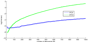
Kernel PCA vs IPCA. We compared kernel PCA features and IPCA left features on the (ii) $2$ circles data. We fixed $M=12$ as the number of feature spanning points, and computed principal components for $N=10,20,\dots,1000$ data points. The six non-degenerate principal vectors and their principal values were equal to the IPCA left feature vectors and the squares of the corresponding singular values, up to machine precision. Figure 1 shows log-runtimes in comparison. The runtime for IPCA is lower by orders of magnitude.

Figure 1: Runtime of kernel PCA and IPCA. Thick line is mean, dotted lines are 0.1 and 0.9 quantiles over $20$ repetitions.

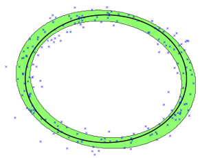
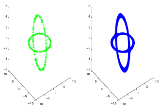
Manifold learning with cross-kernel and IPCA. We used IPCA to learn the data manifold from 200 samples in the (i) circle and the (ii) 2 circle example. The manifold is the approximated by the points with low evaluation of the normalized IPCA certifying features, the result can be seen in figure 2. The singular value threshold was fixed to $m=5$ for (i) and $m=9$ for (ii). The certifying features were evaluated on a fine grid, grid points with evaluation norm near the training data were considered in-manifold, with 0.1-quantile for (i) and 0.01-quantile for (ii).

Figure 2: Manifold estimation with IPCA. The crosses are the data points. The estimated manifolds are the light green ring in 2 and the two blue rings in 2.

Classification with IPCA certifying vectors. We used the IPCA features for classification on the USPS data set. In all experiments, $700$ training examples are used, and the rest of the USPS data set is used for evaluation.

Denote the different training classes $X_{1},\ldots,X_{t}$ and the pooled data by $X_{\text{train}}:=\cup_{i=1}^{t}X_{i}$. The natural form of a one-vs-all classifier using IPCA certifying features is as follows: (1) to train, compute $\operatorname{IPCA}(X_{i},Z)$ for each of the $X_{i}$ with the same fixed $Z$; to classify a set of points $X_{\text{test}}$, compute the right-evaluation vectors using Algorithm 2 for each class and assign the label corresponding to the minimum norm evaluation. The correctness of this construction follows directly from Theorem 3.3. All the stability and convergence guarantees of IPCA go through without modification.

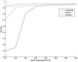
We compare three choices for the feature generating points $Z$: (1) choose the feature-generating matrix $Z$ with standard normal Gaussian entries; (2) choose it as a uniform random sub-sample of $X_{\text{train}}$; (3) choose it as a degenerate sub-sample of $X_{\text{train}}$; we simulate a high number of repetitions by sub-sampling from a sub-sample of size $N/4$.

Figure 3(a) summarizes the results. Non-degenerate sub-sampling (2) is best, since it takes advantage of the implicit dimension-reduction of expressing the $\mathcal{X}_{i}$ in a coordinate system derived $\mathcal{X}\subset\mathbb{R}^{n}$, which can be of much lower dimension than $n$. However, when the sampling is degenerate as in (3), e.g., with many repetitions, a random feature-generating matrix of the same size as in (1) gives better performance. Eventually, with growing $M$ all choices of $Z$ yield comparable results. As it can not be distinguished a-priori whether the training sample is degenerate or not, random $Z$ can be preferrable.

We also compared the IPCA certifying features to the IPCA left and right principal features (PCA-like), by extracting $m=32$ features, then performing linear classification via LIBLINEAR [3]. The feature-generating matrix $Z$ is chosen randomly with standard normal entries. Figure 3(b)–(c) show that $m=32$ certifying features yields more accurate and faster results than the same number of principal features. The results reported in [5] for classical kernel PCA are comparable to the PCA-like features, which all are outperformed by the IPCA certifying features.

Figure 3: (a) Classification with IPCA certifying features, comparing random $Z$ and subsampled $Z$ from generic and degenerate sampling; (b) performance comparison of the three IPCA features - left and right principal features are closely related to kernel PCA features; (c) speed comparison of IPCA feature based classifiers.

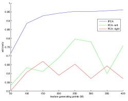
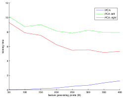
Above comparing different modes of instanciating IPCA, the experiments also show that IPCA is capable of extracting competitive features for considerably less and better scaling computational cost than kernel PCA, and achieves comparable performance on a much smaller number of relevant features.

Acknowledgments

LT is supported by the European Research Council under the European Union’s Seventh Framework Programme (FP7/2007-2013) / ERC grant agreement no 247029-SDModels. This research was conducted while MK and LT were guests of FK at Mathematisches Forschungsinstitut Oberwolfach, supported by FK’s Oberwolfach Leibniz Fellowship.

References

Appendix

• (of Proposition 2.3)
  Let $m=\binom{n+d}{d}$. Under the isomorphism $\mathbb{R}[\mathbf{t}]_{\leq d}\rightarrow\mathbb{R}^{m}$ given by $\sum_{\alpha}c_{\alpha}\mathbf{t}^{\alpha}\mapsto(c_{\alpha})_{|\alpha|\leq d}$, the polynomial $\mathbf{k}_{\leq d}(x,\mathbf{t})$ maps to $(\gamma_{\alpha}^{2}x^{\alpha})_{|\alpha|\leq d}$ for every $x\in\mathbb{R}^{n}$. Up to scaling the coordinates by $\gamma_{\alpha}^{2}$, the image of this isomorphism is a Veronese variety. Now the claim follows from the fact that this Veronese variety is irreducible and non-degenerate. ∎

• (of Proposition 2.4)
  First we show (a). Both vector spaces have the same dimension. The map $\varphi$ is $\mathbb{R}$-linear and sends the basis vector ${\mathbf{t}}^{\alpha}$ to the basis vector $(1/\gamma_{\alpha})\cdot e_{\alpha}^{\ast}$, i.e., to the map defined by $e_{\beta}\mapsto(1/\gamma_{\alpha})\,\delta_{\alpha\beta}$. From this the claim follows.

  To prove (b), we use the standard scalar product on $\mathcal{F}_{\leq d}$ to identify it with $(\mathcal{F}_{\leq d})^{\vee}$. This (non-canonical) isomorphism identifies the standard basis vector $e_{\alpha}$ with $e_{\alpha}^{\ast}$. Thus the claim follows from (a). ∎

• (of Corollary 2.5)
  It is easy to check that $\Phi_{\leq d}^{\ast}=\mathop{\rm eval}\nolimits\circ\varphi^{-1}$. Since both maps $\mathop{\rm eval}\nolimits$ and $\varphi^{-1}$ are isomorphisms, the claim follows. ∎

• (of Proposition 2.6)
  This follows by writing $f=\sum_{\alpha}c_{\alpha}\mathbf{t}^{\alpha}$ with $c_{\alpha}\in\mathbb{R}$ and computing

  $$\langle f,\mathbf{k}_{\leq d}(x,\mathbf{t})\rangle_{\varphi}\;=\;\langle{\textstyle\sum_{\alpha}}c_{\alpha}\mathbf{t}^{\alpha},\,{\textstyle\sum_{\beta}}\gamma_{\beta}^{2}x^{\beta}\mathbf{t}^{\beta}\rangle_{\varphi}\;=\;{\textstyle\sum_{\alpha}}c_{\alpha}\gamma_{\alpha}^{2}x^{\alpha}\langle\mathbf{t}^{\alpha},\mathbf{t}^{\alpha}\rangle_{\varphi}\;=\;{\textstyle\sum_{\alpha}}c_{\alpha}x^{\alpha}\;=\;f(x)$$

  ∎

• (of Theorem 2.8)
  Part (a) follows from the definition of ${\rm I}(\mathcal{X})$ and Prop. 2.6.

  To prove (b), we first use (a) in order to map ${\rm I}(\mathcal{X})_{\leq d}$ isomorphically into $(\mathcal{F}_{\leq d})^{\vee}$. The result is the orthogonal complement of $U=\langle\sum_{|\alpha|\leq d}\gamma_{\alpha}x^{\alpha}e_{\alpha}^{\vee}\mid x\in\mathcal{X}\rangle$. Since we are using the standard scalar products on $\mathcal{F}_{\leq d}$ and its dual, this orthogonal complement equals the annihilator of the preimage of $U$ in $\mathcal{F}_{\leq d}$. That preimage is generated by the elements $\sum_{|\alpha|\leq d}\gamma_{\alpha}x^{\alpha}e_{\alpha}=\Phi_{\leq d}(x)$ with $x\in\mathcal{X}$. In other words, the vector space $U^{\perp}$ is the annihilator of the feature span of $\mathcal{X}$, as claimed.

  Finally, we note that (c) follows from (b) by identifying $\mathcal{F}_{\leq d}$ with its dual via the standard scalar product. ∎

• (of Theorem 3.3)
  First we prove claim (a). Letting $v_{i}=\Phi_{\leq d}(x_{i})\in\mathbb{R}^{m}$ and $w_{j}=\Phi_{\leq d}(z_{j})\in\mathbb{R}^{m}$ for $i=1,\dots,N$ and $j=1,\dots,M$, we have to show that the rank of the matrix $G=(\langle v_{i},w_{j}\rangle)_{i,j}$ equals the dimension of $\langle v_{1},\dots,v_{N}\rangle$. By removing columns and rows of $G$, we may assume that $\{v_{1},\dots,v_{N}\}$ and $\{w_{1},\dots,w_{M}\}$ are linearly independent. Using the hypothesis $\langle v_{1},\dots,v_{N}\rangle\subseteq\langle w_{1},\dots,w_{M}\rangle$, we see that $M\geq N$ and may assume $v_{i}=w_{i}$ for $i=1,\dots,N$. Then the first $N$ columns of $G$ are the Gram matrix of $V=(v_{1},\dots,v_{N})$ and the claim follows from the fact that the rank of the Gram matrix of $V$ equals the rank of $V$.

  Next we show (b). The implication “$\Leftarrow$” is trivially true. To prove the converse, we note that the hypothesis implies that there are $a_{1},\dots,a_{N}\in\mathbb{R}$ such that $\Phi_{\leq d}(c)-\sum_{i=1}^{N}a_{i}\Phi_{\leq d}(x_{i})$ is orthogonal to $\operatorname{fspan}(Z)$. Since this vector is contained in $\operatorname{fspan}(Z)$, it is zero. To prove the additional claim, we note that $\Phi_{\leq d}(c)\in\operatorname{fspan}(X)$ implies that all linear forms in the annihilator of $\operatorname{fspan}(X)$ vanish at $c$. Via $\varphi^{-1}$, these linear forms correspond to the polynomials in ${\rm I}(\mathcal{X})_{\leq d}$. Since $\mathcal{X}$ is cut out by these polynomials, we get $c\in\mathcal{X}$, as claimed.

  For the proof of part (c) we use the isomorphism $\varphi$ to write the hypothesis $f\in{\rm I}(\mathcal{Z})_{\leq d}^{\perp}$ as $f=\sum_{j=1}^{M}c_{j}\mathbf{k}_{\leq d}(z_{j},\mathbf{t})$ for some $c_{j}\in\mathbb{R}$. We have $f\in{\rm I}(\mathcal{X})$ if and only if $\varphi(f)$ is orthogonal to $\langle\varphi(\mathbf{k}_{\leq d}(x_{i},\mathbf{t}))\rangle$. Therefore we require that we have

  $$0 \;=\;\langle\varphi(f),\varphi(\mathbf{k}_{\leq d}(x_{i},\mathbf{t}))\rangle\;=\;\langle{\textstyle\sum_{j=1}^{M}}c_{j}{\textstyle\sum_{\alpha}}\gamma_{\alpha}z_{j}^{\alpha}e_{\alpha}^{\vee},\;{\textstyle\sum_{\alpha}}\gamma_{\alpha}x_{i}^{\alpha}e_{\alpha}^{\vee}\rangle$$

  $$\;=\;{\textstyle\sum_{\alpha}}\gamma_{\alpha}^{2}\left({\textstyle\sum_{j=1}^{M}}c_{j}z_{j}^{\alpha}\right)\,x_{i}^{\alpha}$$

  for $i=1,\dots,N$. On the other hand, the entry in position $(i,j)$ of $K_{\leq d}(X,Z)$ is $k_{\leq d}(x_{i},z_{j})=\langle\Phi_{\leq d}(x_{i}),\,\Phi_{\leq d}(z_{j})\rangle=\langle\sum_{\alpha}\gamma_{\alpha}x_{i}^{\alpha}e_{\alpha},\,\sum_{\alpha}\gamma_{\alpha}z_{j}^{\alpha}e_{\alpha}\rangle=\sum_{\alpha}\gamma_{\alpha}^{2}x_{i}^{\alpha}z_{j}^{\alpha}$. Hence $(c_{1},\dots,c_{M})^{\top}$ is in the nullspace of $K_{\leq d}(X,Z)$ if and only if $\sum_{j=1}^{M}\sum_{\alpha}\gamma_{\alpha}^{2}x_{i}^{\alpha}z_{j}^{\alpha}c_{j}=0$ for $i=1,\dots,N$. As we have seen, this is equivalent to $f\in{\rm I}(\mathcal{X})$.

Finally we show (d). Using Theorem 2.8, we see that the hypothesis yields ${\rm I}(\mathcal{X})^{\perp}=\langle\mathbf{k}_{\leq d}(x_{i},\mathbf{t})\mid i=1,\dots,N\rangle$ and ${\rm I}(\mathcal{Z})^{\perp}=\langle\mathbf{k}_{\leq d}(z_{j},\mathbf{t})\mid j=1,\dots,M\rangle$. Therefore there exist numbers $c_{j}\in\mathbb{R}$ such that we have $f=\sum_{j=1}^{M}c_{j}\mathbf{k}_{\leq d}(z_{j},\mathbf{t})$, and the question is whether there exists a representation $f=\sum_{i=1}^{N}a_{i}\mathbf{k}_{\leq d}(x_{i},\mathbf{t})$ with $a_{i}\in\mathbb{R}$. By the hypothesis, the matrix $K_{\leq d}(Z,Z)$ is invertible, since it is the Gram matrix of the full rank matrix $(\Phi_{\leq d}(z_{j}))$. So, knowing $(c_{1},\dots,c_{M})$ is equivalent to knowing

$$(c_{1},\dots,c_{M})\cdot K_{\leq d}(Z,Z)\;=\;\bigl{(}{\textstyle\sum_{\alpha}}\gamma_{\alpha}^{2}\left({\textstyle\sum_{\ell=1}^{M}}c_{\ell}z_{\ell}^{\alpha}\right)\,z_{j}^{\alpha}\bigr{)}_{j}$$

To prove the implication “$\Rightarrow$” we can write the latter tuple as

$$\bigl{(}{\textstyle\sum_{\alpha}}\gamma_{\alpha}^{2}\left({\textstyle\sum_{i=1}^{N}}a_{i}x_{i}^{\alpha}\right)\,z_{j}^{\alpha}\bigr{)}_{j}\;=\;(a_{1},\dots,a_{n})\cdot K_{\leq d}(X,Z)$$

and conclude that $c=(a_{1},\dots,a_{n})\cdot K_{\leq d}(X,Z)\cdot K_{\leq d}(Z,Z)^{-1}$. For the implication “$\Leftarrow$”, we are given the equalities

$${\textstyle\sum_{\alpha}}\gamma_{\alpha}^{2}\left({\textstyle\sum_{\ell=1}^{M}}c_{\ell}z_{\ell}^{\alpha}\right)\,z_{j}^{\alpha}\;=\;{\textstyle\sum_{\alpha}}\gamma_{\alpha}^{2}\left({\textstyle\sum_{i=1}^{N}}a_{i}x_{i}^{\alpha}\right)\,z_{j}^{\alpha}$$

for $j=1,\dots,M$. This means that, for $j=1,\dots,M$, the vectors $\sum_{\ell=1}^{M}\gamma_{\alpha}c_{\ell}z_{\ell}^{\alpha}e_{\alpha}-\sum_{i=1}^{N}\gamma_{\alpha}a_{i}x_{i}^{\alpha}e_{\alpha}$ and $\sum_{j=1}^{M}\gamma_{\alpha}z_{j}^{\alpha}e_{\alpha}$ are orthogonal with respect to the standard scalar product in $\mathcal{F}_{\leq d}$. Thus the first vector is both orthogonal to $\operatorname{fspan}(Z)$ and contained in $\operatorname{fspan}(Z)$, i.e., it is zero. Consequently, we get $\sum_{\ell=1}^{M}c_{\ell}z_{\ell}^{\alpha}=\sum_{i=1}^{N}a_{i}x_{i}^{\alpha}$, and as we have seen, this yields $f\in{\rm I}(\mathcal{X})_{\leq d}^{\perp}$, as claimed. ∎

• (of Theorem 3.4)
  Let $Y\in\mathbb{R}^{(N+M)\times n}$ be the matrix obtained by row concatenating $X$ and $Z$. Observe that, by construction, there are projection matrices $P$ and $Q$ such that $K(X,X)=P\cdot K(Y,Y)\cdot P^{\top}$ and $K(X,Z)=P\cdot K(Y,Y)\cdot Q^{\top}$, as well as $K(Z,Z)=Q\cdot K(Y,Y)\cdot Q^{\top}$.

  To prove the implication “$\Rightarrow$”, we suppose that $\operatorname{fspan}(X)\nsubseteq\operatorname{fspan}(Z)$. By the rank-nullity theorem, this implies $\operatorname{frk}(Y)>\operatorname{frk}(Z)$. Thus Theorem 3.3.a yields $\operatorname{rank}K_{\leq d}(Z,Z)<\operatorname{rank}K_{\leq d}(Y,Y)$. The claim then follows by applying Lemma 5.1 to $A=K_{\leq d}(Y,Y)$ and $B=Q$ and $C=Q^{\top}$.

  For the reverse implication, we first note that $\operatorname{fspan}(X)\subseteq\operatorname{fspan}(Z)$ implies $\operatorname{fspan}(Y)=\operatorname{fspan}(Z)$. Thus we have $\operatorname{frk}(Y)=\operatorname{frk}(Z)$ and Theorem 3.3.a shows $\operatorname{rank}K_{\leq d}(Z,Z)=\operatorname{rank}K_{\leq d}(Y,Y)$. Now the claim follows by applying Lemma 5.1 in the same way as before. ∎

The following Lemma provides the key ingredient for the preceding proof.

Lemma 5.1.

Let $A\in\mathbb{R}^{m\times n}$, let $B\in\mathbb{R}^{n\times k}$, and let $C\in\mathbb{R}^{\ell\times m}$. Then the matrix equality $A=AB(CAB)^{+}CA$ holds if and only if  $\operatorname{rank}A=\operatorname{rank}CAB$.

• First we show the implication “$\Leftarrow$”. Since $\operatorname{rank}CAB=\operatorname{rank}A$, we have $\operatorname{rank}CA=\operatorname{rank}AB=\operatorname{rank}A$, and therefore $\mathop{\rm colspan}\nolimits(CA)=\mathop{\rm colspan}\nolimits(A)$ as well as $\mathop{\rm rowspan}\nolimits(AB)=\mathop{\rm rowspan}\nolimits(A)$. This implies $A=C^{+}CA=ABB^{+}$. The definition of the pseudoinverse yields $CAB=CAB(CAB)^{+}CAB$. Multiplying this equality by $C^{+}$ and $B^{+}$, we get $A=C^{+}CABB^{+}=C^{+}CAB(CAB)^{+}CABB^{+}=AB(CAB)^{+}CA$, as claimed.

  To prove the reverse implication, suppose that $\operatorname{rank}A\neq\operatorname{rank}CAB$. Since the rank of a matrix does not increase by matrix multiplication, we must have $\operatorname{rank}A>\operatorname{rank}CAB$. Since the pseudoinverse of $CAB$ satisfies $\operatorname{rank}(CAB)^{+}=\operatorname{rank}CAB$, we find $\operatorname{rank}A>\operatorname{rank}CAB=\operatorname{rank}(CAB)^{+}\geq\operatorname{rank}\left(AB(CAB)^{+}CA\right)$, in contradiction to the hypothesis. ∎

References

- [1] Mark A. Aizerman, Emmanuel M. Braverman, and Lev I. Rozonoer. Theoretical foundations of the potential function method in pattern recognition learning. In Automation and Remote Control,, number 25 in Automation and Remote Control,, pages 821–837, 1964.
- [2] Bernhard E. Boser, Isabelle M. Guyon, and Vladimir N. Vapnik. A training algorithm for optimal margin classifiers. In Proceedings of the 5th Annual ACM Workshop on Computational Learning Theory, pages 144–152. ACM Press, 1992.
- [3] R.-E. Fan, K.-W. Chang, C.-J. Hsieh, X.-R. Wang, and C.-J. Lin. LIBLINEAR: A library for large linear classification. Journal of Machine Learning Research 9:1871–1874, 2008.
- [4] Bernhard Schölkopf and Alexander J Smola. Learning with kernels. MIT Press, 2002.
- [5] Bernhard Schölkopf, Alexander Smola, and Klaus-Robert Müller. Nonlinear component analysis as a kernel eigenvalue problem. Neural computation, 10(5):1299–1319, 1998.
- [6] John Shawe-Taylor and Nello Cristianini. Kernel Methods for Pattern Analysis. Cambridge University Press, New York, 2004.
- [7] Vladimir N. Vapnik. The Nature of Statistical Learning Theory. Springer Verlag, New York, 1995.
- [8] USPS handwritten digits data set A Database for Handwritten Text Recognition Research, J. J. Hull, IEEE PAMI 16(5) 550-554, 1994.