Asymptotically exponential hitting times and metastability:
a pathwise approach without reversibility

Abstract

We study the hitting times of Markov processes to target set $G$, starting from a reference configuration $x_{0}$ or its basin of attraction. The configuration $x_{0}$ can correspond to the bottom of a (meta)stable well, while the target $G$ could be either a set of saddle (exit) points of the well, or a set of further (meta)stable configurations. Three types of results are reported: (1) A general theory is developed, based on the path-wise approach to metastability, which has three important attributes. First, it is general in that it does not assume reversibility of the process, does not focus only on hitting times to rare events and does not assume a particular starting measure. Second, it relies only on the natural hypothesis that the mean hitting time to $G$ is asymptotically longer than the mean recurrence time to $x_{0}$ or $G$. Third, despite its mathematical simplicity, the approach yields precise and explicit bounds on the corrections to exponentiality. (2) We compare and relate different metastability conditions proposed in the literature so to eliminate potential sources of confusion. This is specially relevant for evolutions of infinite-volume systems, whose treatment depends on whether and how relevant parameters (temperature, fields) are adjusted. (3) We introduce the notion of early asymptotic exponential behavior to control time scales asymptotically smaller than the mean-time scale. This control is particularly relevant for systems with unbounded state space where nucleations leading to exit from metastability can happen anywhere in the volume. We provide natural sufficient conditions on recurrence times for this early exponentiality to hold and show that it leads to estimations of probability density functions.

1 Introduction

Hitting times to rare sets, and related metastability issues, have been studied both in the framework of probability theory and statistical mechanics.

A short review of first hitting results is given in sect. 1.1. As far as metastability results are concerned, the story is much more involved due to the fact that metastability can be defined in different ways.

The phenomenon of metastability is given by the following scenario: (i) A system remains “trapped” for an abnormally long time in a state —the metastable phase— different from the eventual equilibrium state consistent with the thermodynamical potentials. (ii) Subsequently, the system undergoes a sudden transition from the metastable to the stable state at a random time.

The mathematical study of this phenomenon has been a standing issue since the foundation of the field of rigorous statistical mechanics. This long history resulted in a number of different approaches, based on non-equivalent assumptions.

The common feature of these mathematical descriptions is a stochastic framework involving a Markovian evolution and two disjoint distinguished sets of configurations, respectively representing metastable and stable states. Rigorously speaking, a statistical mechanical “state” corresponds to a probability measure. The association to sets of configurations corresponds, therefore, to identifying supports of relevant measures. This is a crucial step in which both probabilistic and physical information must be incorporated. Within such framework, the central mathematical issue is the description of the first-exit trajectories leading from an initial metastable configuration to a final stable one. The exit path can be decomposed into two parts:

• an escape path —taking the system to the boundary of the metastable set, which can be thought of as a saddle or a bottleneck: a set with small equilibrium measure which is difficult for the system to reach. —

• and a downhill path —bringing the system into the next stable state. —

Metastable behavior occurs when the time spent in the downhill path is negligible with respect to the escape time. In such a scenario, the overall exponential character of the time to reach stability is, therefore, purely due to the escape part of the trajectory. This implies that the set of metastable states can be considered as a single state in the sense that the first escape turns out to be exponentially distributed as in the case of a single state. Actually this exponential law can be considered as the main feature of metastability.

As noted above the first escape from the metastable set can be seen as the first hitting to a rare set of saddle configurations and this is the strong relation between metastability and first hitting to rare events. However we have to note that the important quantity in metastability is the decay time of the metastable phase so the first hitting to the stable one. In order to reduce this problem to the first hitting to a rare set, the saddle set, one has to individuate this boundary set by investigating in detail the state space.

In metastability literature, the main used tools are renormalization [60, 61], cycle decomposition and large deviations [21, 22, 23, 20, 54, 55, 56, 46, 62] and, lately, potential theoretic techniques [9, 10, 12, 13, 5, 6]. Generally speaking, the focus is more on the exit path and on the mean exit time, while the results on the distribution of the escape time are usually asymptotical and not quantitative as in [2].

At any rate, metastability involves a relaxation from an initial measure to a metastable state, from which the systems undergoes a final transition into stability. To put this two-step process in evidence, the theory must apply to sufficiently general initial states.

This paper is based on the path-wise approach to metastability developed in[20, 54, 55, 56, 46]. This approach has led to a detailed description of exit paths in terms of relevant physical quantities, such as energy, entropy, temperature, etc. In this paper we show how the same approach provides simple and effective estimations of the laws of hitting times for rather general, not necessarily reversible dynamics. Moreover we can consider hitting to more general goals, not necessarily rare sets, so, in metastability language, we do not need to individuate the saddle configurations in order to prove the exponentially of the decay time since we can directly consider as goal the stable state. This can be an important point to apply the theory in very complicated physical contexts where is too difficult a detailed control of the state space.

1.1 First hitting: known results

The stochastic treatment was initially developed in the framework of reliability theory, in which the reference states are called good states and the escaped states are the bad states. The exponential character of good-to-bad transitions —well known from quite some time— is due to the existence of two different time scales: Long times are needed to go from good to bad states, while the return to good states from anywhere —except, perhaps, the bad states— is much shorter. As a result, a system in a good state can arrive to the bad state only through a large fluctuation that takes it all the way to the bad state. Any intermediate fluctuation will be followed by an unavoidable return to the good states, where, by Markovianness, the process starts afresh independently of previous attempts. The escape time is formed, hence, by a large number of independent returns to the good states followed by a final successful excursion to badness that must happen without hesitations, in a much shorter time. The exit time is, therefore, a geometric random variable with extremely small success probability; in the limit, exponentiality follows.

A good reference to this classical account is the short book [43] which, in fact, collects also the main tools subsequently used in the field: reversibility, spectral decomposition, capacity, complete monotonicity. Exponentiality of hitting times to rare events is analyzed, in particular, in Chapter 8 of this book, where regenerative processes are considered.

The tools given in [43] where exploited in [17, 18, 19, 1, 2, 3] to provide sharp and explicit estimates on the exponential behavior of hitting times with means larger than the relaxation time of the chain. For future reference, let us review some results of these papers.

Let $X_{t};\,t\geq 0$ be an irreducible, finite-state, reversible Markov chain in continuous time, with transition rate matrix $Q$ and stationary distribution $\pi$. The relaxation time of the chain is $R=1/{\lambda}_{1}$, where ${\lambda}_{1}$ is the smallest eigenvalue of $-Q$. Let ${\tau}_{A}$ denote the hitting time of a given subset $A$ of the state space and ${\mathbb{P}}_{\pi}$ the law of the process started at $\pi$. Then, for all $t>0$ (Theorem 1 in [2]):

$$\Bigl{|}{\mathbb{P}}_{\pi}\bigl{(}{\tau}_{A}/{\mathbb{E}}_{\pi}{\tau}_{A}>t\bigr{)}-e^{-t}\Bigr{|}\;\leq\;{R/{\mathbb{E}}_{\pi}{\tau}_{A}\over 1+R/{\mathbb{E}}_{\pi}{\tau}_{A}}\;.$$ (1.1)

Moreover in the regime $R\ll t\ll{\mathbb{E}}_{\pi}{\tau}_{A}$, the distribution of ${\tau}_{A}$ rescaled by its mean value, can be can be controlled with explicit bounds on its density function (Sect. 7 of [2]). We note that these results are given in terms of quantitative estimates which are strict when $R/{\mathbb{E}}_{\pi}{\tau}_{A}\ll 1$ and the starting distribution is the equilibrium measure.

Further insight is provided by the quasi-stationary distribution

$${\alpha}\;:=\;\lim_{t\to\infty}{\mathbb{P}}_{\pi}(X_{t}\in\cdot\mid{\tau}_{A}>t)\;.$$

This distribution is stationary for the conditional process

$${\alpha}\;=\;{\mathbb{P}}_{\alpha}(X_{t}\in\cdot\mid{\tau}_{A}>t)\;,$$

and starting from ${\alpha}$ the hitting time to $A$ is exponential with rate $1/{\mathbb{E}}_{\alpha}{\tau}_{A}$. If the set $A$ is such that $R/{\mathbb{E}}_{\pi}{\tau}_{A}$ is small, then the distance between the stationary and quasi-stationary measures is small and, as shown in Theorem 3 of [2],

$${\mathbb{P}}_{\pi}\bigl{(}{\tau}_{A}>t\bigr{)}\;\geq\;\Bigl{(}1-{R\over{\mathbb{E}}_{\alpha}{\tau}_{A}}\Bigr{)}\,\exp\Bigl{\{}-{t\over{\mathbb{E}}_{\alpha}{\tau}_{A}}\Bigr{\}}\;.$$ (1.2)

The proofs of these results are based on the property of complete monotonicity derived from the spectral decomposition of the transition matrix restricted to the complement of $A$.

While reversibility has been crucially exploited in all these proofs, there exist another representation for first hitting times, always due to [19], based on the famous interlacing eigenvalues theorem of linear algebra. This representation has been very recently re-derived, using a different approach, [33] who use it to the generalize the results to non reversible chains.

While the previous formulas are very revealing, they are restricted to the situations in which the “good” reference state is the actual equilibrium measure.

The common feature of these approaches is their central use of the invariant measure both as a reference and to compute the corrections to exponential laws. As this object is generally unknown and hard to control, the resulting theories lead to hypotheses and criteria not easy to verify.

An higher level of generality is achieved by the martingale approach recently applied in [7] to obtain results comparable to those in theorem 2.7 below. In this reference, however, exponential laws are derived for visits to rare sets —that is, sets with asymptotically small probability. In metastability or reliability theory this corresponds to visits to the saddles mediating between good and bad or between stable and metastable states. As mentioned above, we recall that the approach proposed in the present paper does not require the determination of these saddle states, and exponential laws are derived also for visit to sets $G$ including the stable state. Moreover, in this work we concentrate on recurrence hypotheses defined purely in terms of the stochastic evolution with no reference to an eventual invariant state.

1.2 Metastability: A few key settings.

Having in mind different asymptotic regimes, many different definitions of metastable states have been given in the literature. These notions, however, are not completely equivalent as they rely on different properties of hitting and escape times. This state of affairs makes direct comparisons difficult and may lead to confusion regarding applicability of the different theories to new problems.

Since metastability is always associated with a particular asymptotic regime, the results given in the literature are always given in asymptotic form.

In order to understand the reasons behind the different notions of metastability, it is useful to survey the main situations where metastability has been studied.

The simplest case is when the system recurs in a single point. The main asymptotic regimes that fall into this class are:

• Finite state space in the limit of vanishing transition probabilities. Typical examples are lattice systems, with short range interaction, Glauber [4, 16, 25, 27, 29, 44, 45, 49, 52, 53, 57, 58](or Kawasaki[14, 37, 38, 39, 40, 41, 42, 50], or parallel[8, 23, 26, 28, 27, 51, 62, 63]) dynamics, in the limit of vanishing temperature. In this regime, the transition probabilities between neighbour points $x$ and $y$ have the form $P(x,y)=\exp(-{\beta}{\Delta}H(x,y))$, where $\beta\to\infty$ is the inverse temperature and ${\Delta}H(x,y)$ is the energy barrier between $x$ and $y$.
  In this regime, the escape pattern can be understood in terms of the energy landscape (more generally, in terms of the equilibrium measure). The mean exit time scales as $\exp(-{\beta}\Gamma)$, where $\Gamma$ is the energy barrier between the metastable and the stable configurations.

• Finite transition probabilities in the limit of diverging number of steps to attain stability. The typical example of this regime regards mean field models [11, 20]. Indeed, these systems can be mapped into a low-dimensional Markov process recurring in a single point and where metastability can be described in terms of free–energy landscape. The mean exit time scales as $\exp(-n\Delta)$, where $n\to\infty$ is the volume and $\Delta$ is the free-energy barrier divided by the temperature.

  The kinetic Ising model at finite temperature in the limit of vanishing magnetic field $h$ in a box of side-length $1/h$ is another example of this class (see [59]), since the critical droplet becomes larger and larger as $h$ tends to $0$.

  Many toy models, including the one–dimensional model discussed in section 5.2.2, pertain to this regime.

In the rest of the subsection we will discuss some cases where metastability can be described in terms of entropic corrections of the regimes above.

For instance, suppose to have many independent copies of a system in the regime of finite state space and vanishing transition probabilities, and that the target event is the hitting to a particular set in any of the copies. Physical phenomena of this kind are bolts (discharge of supercharged condensers) and ”homogeneous nucleation” in short range thermodynamic systems (i.e. the formation of the first critical nucleus in a large volume) [15, 42, 35, 31, 59] Since the target event can take place in any of the subsystems, the hitting time is shortened with respect to a single subsystem and, in general, its law changes. This regime is the physical motivation behind our notion of ”early behavior” (see definition 2.9 below).

A wonderful example where the entropic correction is related to fine details of the dynamics is given by the ”nucleation and growth models” (see e.g. [30, 31, 24, 47, 48, 59]), where the transition to stability is driven by the formation, the growth and eventually the coalescence of critical droplets. In these systems the mean relaxation time is the sum of the ”nucleation time” in a ”critical volume”, which is often exponentially distributed, and the ”travel time” needed for two neighbor droplets to grow and coalesce (which, at least in some systems, is believed to have a cut-off behavior).

For general Markov chains, however, metastability cannot be understood in terms of the invariant measure landscape. The system is trapped in the metastable state both because of the hight of the saddles and the presence of bottlenecks and there is not a general recipe to analyze this situation. The results given in this paper allow to deal with the cases where the system recurs in a single point. In a forthcoming paper, we will deal with the general case, where recurrence to the ”quasi–stationary measure” (or to a sufficiently close measure) is used.

In section 2.3, we compare the different definitions of metastability that have been given in the literature for different asymptotic regimes.

1.3 Goal of the paper

The goal of this paper is twofold. First, we develop an overall approach to the study of exponential hitting times which, we believe, is at the same time general, natural and computationally precise. It is general because it does not assume reversibility of the process, does not assume that the hitting is to a rare event and does not assume a particular starting measure. It is natural because it relies on the most universal hypothesis for exponential behavior —recurrence— without any further mathematical assumptions like complete monotonicity or other delicate spectral properties of the chain. Furthermore, the proofs are designed so to follow closely physical intuition. Rather than resorting to powerful but abstract probabilistic or potential theoretical theorems, each result is obtained by comparing escape and recurrence time scales and decomposing appropriately the relevant probabilities. Despite its mathematical simplicity, the approach yields explicit bounds on the corrections to exponentiality, comparable to Lemma 7 of [2] but without assuming initial equilibrium measure.

A second goal of the paper is to compare and relate metastability conditions proposed in the literature [9, 11, 46]. Indeed, different authors rely on different definitions of metastable states involving different hypotheses on hitting and escape times. The situation is particularly delicate for evolutions of infinite-volume systems, whose treatment depends on whether and how relevant parameters (temperature, fields) are adjusted as the thermodynamic limit is taken. We do a comparative study of these hypotheses to eliminate a potential source of confusion regarding applicability of the different theories to new problems.

A further contribution of our paper is our notion of early asymptotic exponential behavior (Definition 2.11) to control the exponential behavior on a time scale asymptotically smaller than the mean-time scale. This notion is particularly relevant for systems with unbounded state space where it leads to estimations of probability density functions. Furthermore, as discussed below, this strong control of exponentiality at small times is important to control infinite-volume systems in which the nucleations leading to exit from metastability can happen anywhere in the volume. We provide natural sufficient conditions on recurrence times for this early exponentiality to hold.

The main limitation of our approach —shared with the majority of the metastability literature— is the assumption that recurrence refers to the visit to a particular configuration. Actually this particular configuration $x_{0}$ can be chosen quite arbitrarily in the ”metastable well”. A more general treatment, involving extended metastable measures for which it is not possible to speak of metastable well, is the subject of current research ([32]).

We conclude this section with the outline of the paper. In section 2 we give main definitions, results on the exponential behavior and compare different hypothesis used in the literature with the ones used in this paper. In section 3 we give some key lemmas that are used in section 4 to prove the main theorems about the exponential behavior. In section 5 we prove the results about the comparison of different hypothesis and we give an example that depending on the values of parameters fulfills different hypothesis to show that in general they are not all equivalent. The appendix contains computations of quantities needed in the example.

2 Results

2.1 Models and notation

We consider a family of discrete time irreducible Markov chains with transition matrices $P^{(n)}$ and invariant measures $(\pi^{(n)},\,n\geq 1)$ on finite state spaces $({\cal X}^{(n)},\,n\geq 1)$. A particular interesting case is the infinite volume asymptotics $\lim_{n\to\infty}|{\cal X}^{(n)}|=\infty$.

We use scriptless symbols ${\mathbb{P}}(\cdot)$ and ${\mathbb{E}}(\cdot)$ for probabilities and expectations while keeping the parameter $n$ and initial conditions as labels of events and random variables. In particular $X^{(n),x}=\bigl{(}X^{(n),x}_{t}\bigr{)}_{t\in\mathbb{N}}$ denotes the chain starting at $x\in{\cal X}^{(n)}$, and the hitting time of a set $F^{(n)}\subset{\cal X}^{(n)}$ is denoted by

$${\tau}^{(n),x}_{F^{(n)}}=\inf\Bigl{\{}t\geq 0:\;X^{(n),x}_{t}\in F^{(n)}\Bigr{\}}$$ (2.3)

For guidance we use uppercase latin letters for sequences of diverging positive constants, and lowercase latin letters for numerical sequences converging to zero when $n\to\infty$. The small-o notation $o_{n}(1)$ indicates a sequence of functions going uniformly to $0$ as $n\to\infty$. The symbol $A_{n}\succ B_{n}$ indicates, $B_{n}/A_{n}=o_{n}(1)$.

The notation $X=\bigl{(}X_{t}\bigr{)}_{t\in\mathbb{N}}$ is used for a generic chain on ${\cal X}$. Quantitave results will be given for such a generic chain, while asymptotical results are given for the sequence $X^{(n)}$. The shorter notation without superindex $(n)$ is also used in proofs where result are discussed for a single choice of $n$.

2.2 General results on exponential behavior

The general setup in the sequel comprises some ingredients. First, a point $x_{0}$ thought of as a(meta)stable state. In reversible chains, such a point corresponds to the bottom of an “energy well” or, more generally, to a given state in the energy well. In our treatment, it is irrelevant whether it corresponds to an absolute (stable) or local (metastable) energy minimum. The second ingredient is a non empty set $G$ of points marking the exit from the “well”. Depending on the application, this set can be formed by exit points, by saddle points, by the basin of attraction of the stable points or by the target stable points. The random time ${\tau}_{G}^{x_{0}}$, i.e., the first hitting time to $G$ starting from $x_{0}$, corresponds therefore to the exit time or transition time in the metastable setting. We call $(x_{0},G)$ a reference pair.

We characterize the scale of return times (renewal times) by means of two parameters:

Definition 2.1

Let $R>0$ and $r\in(0,1)$, we say that a reference pair $(x_{0},G)$ satisfies $Rec(R,r)$ if

$$\sup_{x\in{\cal X}}{\mathbb{P}}\Bigl{(}{\tau}_{\{x_{0},G\}}^{x}>R\Bigr{)}\;\leq\;r\;.$$ (2.4)

We will refer to $R$ and $r$ as the recurrence time and recurrence error respectively. The hitting time to $\{x_{0},G\}$ is one of the key ingredients of our renewal approach.

Definition 2.2

Given a reference pair $(x_{0},G)$ and $r_{0}\in(0,1)$, we define the basin of attraction of $x_{0}$ of confidence level $r_{0}$ the set

$$B(x_{0},r_{0}):=\{x\in{\cal X};\;{\mathbb{P}}({\tau}^{x}_{\{x_{0},G\}}={\tau}^{x}_{x_{0}})>1-r_{0}\}$$ (2.5)

Theorem 2.3

Consider a reference pair $(x_{0},G)$, with $x_{0}\in{\cal X}$, $G\subset{\cal X}$, such that $Rec(R,r)$ holds with $R<T:={\mathbb{E}}{\tau}_{G}^{x_{0}}$, with ${\varepsilon}:={R\over T}$ and $r$ sufficiently small. Then, there exist functions $C(\epsilon,r)$ and $\lambda(\epsilon,r)$ with

$$C(\epsilon,r)\;,\;\lambda(\epsilon,r)\;\longrightarrow\;0\quad\mbox{as}\quad\epsilon,r\,\to\,0\;,$$ (2.6)

such that

$$\Big{|}{\mathbb{P}}\Big{(}{{\tau}_{G}^{x_{0}}\over T}>t\Big{)}-e^{-t}\Big{|}\;\leq\;C\,e^{-(1-\lambda)\,t}$$ (2.7)

for any $t>0$. Furthermore, there exist a function $\widetilde{C}(\epsilon,r,r_{0})$ with

$$\widetilde{C}(\epsilon,r,r_{0})\to 0\quad\mbox{as}\quad\epsilon,r,r_{0}\,\to\,0\;,$$ (2.8)

such that, for any $z\in B(x_{0},r_{0})$,

$$\Big{|}{\mathbb{P}}\Big{(}{{\tau}_{G}^{z}\over T}>t\Big{)}-e^{-t}\Big{|}\;\leq\;\widetilde{C}\,e^{-(1-\lambda)\,t}$$ (2.9)

Remarks 2.4

As already discussed in the Introduction, similar results are given in the literature both in the field of first hitting to rare events and in the field of escape from metastability. We have to stress here that we are not assuming reversibility and we have quite general assumptions on starting condition.

Metastability studies involve sequences of Markov chains on a sequence of state spaces ${\cal X}^{(n)}$.

Definition 2.5

A sequence of reference pairs $\bigl{(}x_{0}^{(n)},G^{(n)}\bigr{)}$, with $x_{0}^{(n)}\in{\cal X}^{(n)}$, $\emptyset\neq G^{(n)}\subset{\cal X}^{(n)}$ satisfies Hypothesis Hp.$G(T_{n})$ for some increasing positive sequence $(T_{n})$ if there exist sequences $r_{n}=o_{n}(1)$ and $R_{n}\prec T_{n}$ such that the recurrence property $Rec(R_{n},r_{n})$ holds in the following sense:

$$\sup_{x\in{\cal X}^{(n)}}{\mathbb{P}}\Bigl{(}{\tau}_{\{x_{0}^{(n)},G^{(n)}\}}^{(n),x}>R_{n}\Bigr{)}\;\leq\;r_{n}\;.$$ (2.10)

Definition 2.6

Given a sequence of reference pairs $(x_{0}^{(n)},G^{(n)})$ and a sequence $r^{(n)}_{0}\to 0$, we define the basin of attraction of $x^{(n)}_{0}$ of confidence level $r^{(n)}_{0}$ the set

$$B(x^{(n)}_{0},r^{(n)}_{0}):=\{x\in{\cal X}^{(n)};\;{\mathbb{P}}({\tau}^{x}_{\{x_{0}^{(n)},G\}}={\tau}^{x}_{x_{0}^{(n)}})>1-r^{(n)}_{0}\}$$ (2.11)

We have the following exponential behaviour for the first hitting time to $G^{(n)}$:

Theorem 2.7

Consider a sequence of reference pairs $\bigl{(}x_{0}^{(n)},G^{(n)}\bigr{)}$ with mean exit times

$$T_{n}^{E}:={\mathbb{E}}\Bigl{(}{\tau}_{G^{(n)}}^{(n),x_{0}^{(n)}}\Bigr{)}$$ (2.12)

and $\zeta$-quantiles information time

$$Q_{n}(\zeta):=\inf\Bigl{\{}k\geq 1\,:\,{\mathbb{P}}\Bigl{(}{\tau}_{G^{(n)}}^{(n),x_{0}^{(n)}}\leq k\Bigr{)}\geq 1-\zeta\Bigr{\}}.$$ (2.13)

Then,

• If Hp.$G(T_{n}^{E})$ holds:

  • ${\tau}_{G^{(n)}}^{(n),x_{0}^{(n)}}/T_{n}^{E}$ converges in law to an $\exp(1)$ random variable, that is,

    $$\lim_{n\to\infty}{\mathbb{P}}\Bigl{(}{\tau}_{G^{(n)}}^{(n),x_{0}^{(n)}}>t\,T_{n}^{E}\Bigr{)}\;=\;e^{-t}\;.$$ (2.14)

  • Furthermore,

    $$\lim_{n\to\infty}\sup_{x\in B(x^{(n)}_{0},r^{(n)}_{0})}\Big{|}{\mathbb{P}}\Bigl{(}{\tau}_{G^{(n)}}^{(n),x}>t\,T_{n}^{E}\Bigr{)}\;-\;e^{-t}\Big{|}=0$$ (2.15)

• If Hp.$G(Q_{n}(\zeta))$ holds:

  • ${\tau}_{G^{(n)}}^{(n),x_{0}^{(n)}}/Q_{n}(\zeta)$ converges in law to an $\exp(-\ln\zeta)$ random variable, that is,

    $$\lim_{n\to\infty}{\mathbb{P}}\Bigl{(}{\tau}_{G^{(n)}}^{(n),x_{0}^{(n)}}>t\,Q_{n}(\zeta)\Bigr{)}\;=\;\zeta^{t}\;.$$ (2.16)

  • The rates converge,

    $$\lim_{n\to\infty}{Q_{n}(\zeta)\over T_{n}^{E}}=-\ln\zeta$$ (2.17)

A popular choice for the parameter $\zeta$ in the quantile is $e^{-1}$. In this case all rates are equal to $1$. For our purposes all choices will work.

Under weaker hypotheses on $T_{n}$, we can prove exponential behavior in a weaker form:

Corollary 2.8

If $T_{n}$ is a sequence of times such that

$$\exists\,\zeta<1\,:\,P\Bigl{(}{\tau}_{G^{(n)}}^{(n),x_{0}^{(n)}}>\,T_{n}\Bigr{)}\geq\zeta\mbox{ uniformly in }n$$

and if Hp.$G(T_{n})$ holds, then the sequence ${\tau}_{G^{(n)}}^{(n),x_{0}^{(n)}}/{\mathbb{E}}\Bigl{(}{\tau}_{G^{(n)}}^{(n),x_{0}^{(n)}}\Bigr{)}$ converges in law to an exp(1) random variable. Indeed in this case we have $T_{n}\leq Q_{n}(\zeta)$ so that Hp.$G(T_{n})$ implies Hp.$G(Q_{n}(\zeta))$.

Notice that recurrence to a single point is not necessary to get exponential behavior of the hitting time. A simple example where we get exact exponential behavior independently of the initial distribution is when the one-step transition probability $P_{x,G}$ is constant for $x\in G^{c}$.

As explained in the introduction there are situations, e.g., when treating metastability in large volumes, that call for more detailed information on a short time scale on hitting times.

Definition 2.9

A random variable $\theta$ has early exponential behaviour at scale $S\leq{\mathbb{E}}\theta$ with rate ${\alpha}$, if for each $k$ such that $kS\leq{\mathbb{E}}\theta$ we have

$$\Big{|}{{\mathbb{P}}\bigl{(}\theta\in(kS,(k+1)S]\bigr{)}\over{\mathbb{P}}(\theta>S)^{k}\,\,{\mathbb{P}}(\theta\leq S)}-1\Big{|}<{\alpha}.$$ (2.18)

We denote this behavior by $EE(S,{\alpha})$.

Remark 2.10

A remark on the difference between the notion of early exponential behaviour and the exponential behaviour given by Theorem 2.3 is necessary. Early exponential behaviour controls the distribution only on short times, $kS<{\mathbb{E}}\theta$, while equation (2.7) holds for any $t$. However on the first part of the distribution EE$(S,{\alpha})$ can give a more detailed control on the density of the distribution. More precisely if ${\tau}_{G}^{x_{0}}$ is EE$(S,{\alpha})$ with ${\alpha}$ small, we can obtain estimates on the density $f(t)$ of ${\theta\over{\mathbb{E}}\theta}$, equivalent to the results obtained in [2], Lemma 13, (a),(b). Indeed

$${\mathbb{P}}\bigl{(}{\tau}_{G}^{x_{0}}\in(kS,(k+1)S]\bigr{)}\;=\;e^{-{\lambda}k}(1-e^{-{\lambda}})(1+a_{k})$$

where $\lambda:=-\ln{\mathbb{P}}({\tau}_{G}^{x_{0}}>S)$ and

$$a_{k}\;:=\;{{\mathbb{P}}\bigl{(}{\tau}_{G}^{x_{0}}\in(kS,(k+1)S]\bigr{)}\over{\mathbb{P}}({\tau}_{G}^{x_{0}}>S)^{k}\,\,{\mathbb{P}}({\tau}_{G}^{x_{0}}\leq S)}-1$$

The absolute value of $a_{k}$ is bounded by $\alpha$ if EE$(S,{\alpha})$ holds uniformly in $k<\frac{{\mathbb{E}}{\tau}_{G}^{x_{0}}}{S}$. In the case $S\ll{\mathbb{E}}{\tau}_{G}^{x_{0}}$, Lemma 3.3 below implies that $\lambda\sim{S\over{\mathbb{E}}{\tau}_{G}^{x_{0}}}$. Thus,

$$f\Bigl{(}k{S\over{\mathbb{E}}{\tau}_{G}^{x_{0}}}\Bigr{)}\,{S\over{\mathbb{E}}{\tau}_{G}^{x_{0}}} \sim {\mathbb{P}}\Bigl{(}{{\tau}_{G}^{x_{0}}\over{\mathbb{E}}{\tau}_{G}^{x_{0}}}\in(k{S\over{\mathbb{E}}{\tau}_{G}^{x_{0}}},(k+1){S\over{\mathbb{E}}{\tau}_{G}^{x_{0}}}]\Bigr{)}$$ (2.19)

$$= e^{-{\lambda}k}(1-e^{-{\lambda}})(1+a)$$

$$\sim e^{-{S\over{\mathbb{E}}{\tau}_{G}^{x_{0}}}k}\,\Bigl{[}{S\over{\mathbb{E}}{\tau}_{G}^{x_{0}}}+o\Bigl{(}{S\over{\mathbb{E}}{\tau}_{G}^{x_{0}}}\Bigr{)}\Bigr{]}\,\bigl{(}1+a\bigr{)}$$

Definition 2.11

A family of random variables $(\theta_{n})_{n}$ with ${\mathbb{E}}\theta_{n}\to\infty$ for $n\to\infty$, has an asymptotic early exponential behaviour at scale $(S_{n})_{n}$ if for every integer $k$

$$\lim_{n\to\infty}{{\mathbb{P}}\bigl{(}\theta_{n}\in(kS_{n},(k+1)S_{n}]\bigr{)}\over{\mathbb{P}}(\theta_{n}>S_{n})^{k}\,\,{\mathbb{P}}(\theta_{n}\leq S_{n})}=1$$ (2.20)

Remark 2.12

The notion of $EE(S_{n},{\alpha})$ is interesting for ${\alpha}$ small and when $S_{n}$ is asymptotically smaller than ${\mathbb{E}}(\theta_{n})$ so that ${\mathbb{P}}(\theta_{n}\leq S_{n})\to 0$ as $n\to\infty$. The sharpness condition (2.20) controls the smallness of these probabilities. In particular it implies that

$$\frac{{\mathbb{P}}(\theta_{n}\leq kS_{n})}{1-{\mathbb{P}}(\theta_{n}>S_{n})^{k}}\;\mathrel{\mathop{\kern 0.0pt\hbox to34.1433pt{\rightarrowfill}}\limits_{n\rightarrow\infty}^{\;}}1$$ (2.21)

The following theorem determines convenient sufficient conditions for early exponential behaviour at scale.

Theorem 2.13

Given a reference pair $\bigl{(}x_{0},G\bigr{)}$, satisfying $Rec(R,r)$ with $0<R<T:={\mathbb{E}}{\tau}_{G}^{x_{0}}$. Define ${\varepsilon}:={R\over T}$ and suppose ${\varepsilon}$ and $r$ sufficiently small. Then ${\tau}_{G}^{x_{0}}$ has $EE(\eta T,{\alpha})$ with $\alpha=O(\epsilon/\eta)+O(r/\eta)$, for $\eta$ such that $\eta\in(0,1)$, $\epsilon/\eta$ and $r/\eta$ are small enough. For instance the property holds for $\eta=\bigl{[}\max\{\epsilon,r\}\bigr{]}^{\gamma}$ with $\gamma<1$ and $\epsilon,r$ small enough.

The following theorem is an immediate consequence of the previous one.

Theorem 2.14

Consider a sequence $\bigl{(}x_{0}^{(n)},G^{(n)},T_{n}\bigr{)}$, with $x_{0}^{(n)}\in{\cal X}^{(n)}$, $G^{(n)}\subset{\cal X}^{(n)}$ and $T_{n}>0$ satisfying Hypothesis Hp.$G(T_{n})$, with $r_{n}\to 0$. Then the family of random variables ${{\tau}_{G^{(n)}}^{(n),x_{0}^{(n)}}}$ has asymptotic exponential behavior at every scale $S_{n}$ such that

$$r_{n}\prec\;\frac{S_{n}}{T_{n}}\qquad\hbox{ and }\qquad\frac{R_{n}}{T_{n}}\;\prec\;\frac{S_{n}}{T_{n}}\;\leq\;1\;.$$ (2.22)

2.3 Comparison of hypotheses

Many different hypotheses have been used in the literature to prove exponential behavior. In this section we analyze some of these hypotheses in order to clarify the relations between them. The notation 2.5 can be used to discuss different issues, in particular:

• the hitting problem (where $x_{0}$ is the maximum of the equilibrium measure and $G$ is a rare set)

• the exit problem and applications to metastability(where $x_{0}$ is a local maximum of the equilibrium measure, e.g., the metastable state, and $G$ is either the ”saddle”, the basin of attraction of the stable state or the stable state itself)

A key quantity, especially in the ”potential theoretic approach” is the following:

Definition 2.15

$A\subset{\cal X}$ and $z,x\in{\cal X}$ the local time spent in $x$ before reaching $A$ starting from $z$ is

$$\xi^{z}_{A}(x):=\Bigl{|}\Bigl{\{}t<{\tau}^{z}_{A}:\;X^{z}_{t}=x\Bigr{\}}\Bigr{|}.$$ (2.23)

The following hypotheses are instances of Definition 2.5.

Hypotheses I

$$Hp.G^{E}\equiv Hp.G(T_{n}^{E})\quad \hbox{ with }\quad T_{n}^{E}={\mathbb{E}}\Bigl{(}{\tau}_{G^{(n)}}^{(n),x_{0}^{(n)}}\Bigr{)}$$ (2.24)

$$Hp.G^{\zeta}\equiv Hp.G(T_{n}^{Q^{\zeta}})\quad \hbox{ with }\quad T_{n}^{Q^{\zeta}}=\inf\Bigl{\{}t:\;{\mathbb{P}}\Bigl{(}{\tau}^{(n),x_{0}^{(n)}}_{G^{(n)}}>t\Bigr{)}\leq\zeta\Bigr{\}}$$ (2.25)

$$Hp.G^{LT}\equiv Hp.G(T_{n}^{LT})\quad \hbox{ with }\quad T_{n}^{LT}={\mathbb{E}}\Bigl{(}\xi^{(n),x_{0}^{(n)}}_{G^{(n)}}(x_{0}^{(n)})\Bigr{)}$$ (2.26)

We show in Theorem 2.17 below that the first two hypotheses are equivalent for every $\zeta<1$. In particular this shows the insensitivity of metastability studies to the choice of $\zeta$. For $\zeta=e^{-1}$, hypothesis $Hp.G^{1/e}$ is equivalent to the ones considered in previous papers (see for instance [46] hypothesis of Theorem 4.15) to determine the distribution of the escape times for general Metropolis Markov chains in finite volume. The last hypotheses $Hp.G^{LT}$ is new and it is useful to compare the first two hypothesis with the two hypotheses below.

The next set of hypotheses refer to the following quantity.

Definition 2.16

Let

$$\widetilde{\tau}^{{(n)},x}_{A}:=\min\Bigl{\{}t>0:X^{(n),x}_{t}\in A\Bigr{\}}$$ (2.27)

be the first positive hitting time to $A$ starting at $x$.

Given reference pairs $\{x_{0}^{(n)},G^{(n)}\}$, define

$$\rho_{A}(n):=\sup_{z\in{\cal X}^{(n)}\backslash\{x_{0}^{(n)},G^{(n)}\}}{{\mathbb{P}}\Bigl{(}\widetilde{\tau}^{{(n)},x_{0}^{(n)}}_{G^{(n)}}<\widetilde{\tau}^{{(n)},x_{0}^{(n)}}_{x_{0}^{(n)}}\Bigr{)}\over{\mathbb{P}}\Bigl{(}\widetilde{\tau}^{{(n)},z}_{\{x_{0}^{(n)},G^{(n)}\}}<\widetilde{\tau}^{{(n)},z}_{z}\Bigr{)}}$$ (2.28)

and

$$\rho_{B}(n):=\sup_{z\in{\cal X}^{(n)}\backslash\{x_{0}^{(n)},G^{(n)}\}}{{\mathbb{E}}{\tau}^{{(n)},z}_{\{x_{0}^{(n)},G^{(n)}\}}\over{\mathbb{E}}{\tau}^{(n),x_{0}^{(n)}}_{G^{(n)}}}\;.\qquad\qquad$$ (2.29)

Hypotheses II

$$Hp.A:\quad \lim_{n\to\infty}|{\cal X}^{(n)}|\rho_{A}(n)=0\qquad\qquad\qquad$$ (2.30)

$${Hp.B}:\quad \lim_{n\to\infty}\rho_{B}(n)=0\qquad\qquad\qquad$$ (2.31)

When $x_{0}$ is the metastable configuration and $G$ is the stable configuration (more precisely when ${\mathbb{E}}(\xi^{x_{0}}_{G})<{\mathbb{E}}(\xi_{x_{0}}^{G})$ ) $Hp.A$ is similar to the hypotheses considered in [10] while $Hp.B$ is similar to those assumed in [9]. Theorem 1.3 in [12] shows that, under hypothesis $Hp.A$ and reversibility, ${\tau}^{x_{0}}_{G}/{\mathbb{E}}({\tau}^{x_{0}}_{G})$ converges to a mean $1$ exponential variable.

Our last theorem establishes the relation between the previous six hypotheses.

Theorem 2.17

The following implications hold:

$$Hp.A\;\Longrightarrow\;Hp.G^{LT}\;\Longrightarrow\;Hp.G^{E}\;\Longleftrightarrow\;Hp.G^{\zeta}\;\Longleftrightarrow\;Hp.B$$ (2.32)

for any $\zeta<1$. Furthermore, the missing implications are false.

These relations are summarized in Figure 1.

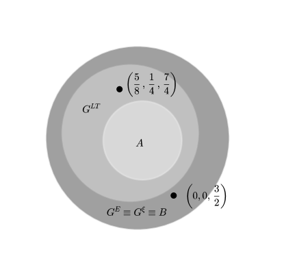
Figure 1: Venn diagram for the conditions in theorem 2.17. The two points correspond to particular choices of the parameters in the ”abc model” stated in section 5.2.2. INGRANDIRE

Remarks 2.18

• Theorem 2.7 holds with either hypothesis $Hp.B$ of the originally stated $Hp.G^{E}$ or $Hp.G^{\zeta}$.

• The first equivalence shows, in particular, that all hypotheses $Hp.G^{\zeta}$ with $\zeta<1$ are mutually equivalent.

• Typically, in metastable systems, for a given target set $G$ there are many possible choices for the point $x_{0}$ to form a reference pair that verifies Hp. B.
  Let $\mathcal{M}_{G}^{\epsilon}:=\left\{x\ ;\;\sup_{z\not\in\left\{x,G\right\}}\mathbb{E}(\tau_{\left\{x,G\right\}}^{z})/\mathbb{E}(\tau_{G}^{x})<\epsilon\right\}$ be the set of all points that toghether with $G$ form a reference pair according to Hp.B.
  If $x,\;y\in\mathcal{M}_{G}^{\epsilon}$, then

  $$\frac{1}{1+\epsilon}\leq\frac{\mathbb{E}(\tau_{G}^{x})}{\mathbb{E}(\tau_{G}^{y})}\leq 1+\epsilon$$ (2.33)

  and

  $$\mathbb{P}\left(\tau_{x}^{y}<\tau_{G}^{y}\right)\geq 1-2\epsilon\ \ \ ;\ \ \ \mathbb{P}\left(\tau_{y}^{x}<\tau_{G}^{x}\right)\geq 1-2\epsilon$$ (2.34)

  Indeed, for any $x,y,z\in\mathcal{X}$,

  $$\mathbb{E}(\tau_{z}^{y}) = \mathbb{E}(\tau_{\left\{x,z\right\}}^{y})+\mathbb{E}(\tau_{z}^{y}-\tau_{\left\{x,z\right\}}^{y})$$ (2.35)

  $$= \mathbb{E}(\tau_{\left\{x,z\right\}}^{y})+\mathbb{E}\left((\tau_{z}^{y}-\tau^{y}_{x}){1}_{\tau_{x}^{y}<\tau_{z}^{y}}\right)$$

  $$= \mathbb{E}(\tau_{\left\{x,z\right\}}^{y})+\mathbb{E}(\tau_{z}^{x})\mathbb{P}\left(\tau_{x}^{y}<\tau_{z}^{y}\right),$$

  where we used strong Markov property at time $\tau_{x}^{y}$ in the last equality.
  When $x\in\mathcal{M}_{G}^{\epsilon}$,

  $$\mathbb{E}(\tau_{G}^{y})\leq\mathbb{E}(\tau_{G}^{x})\left(\epsilon+1\right)$$ (2.36)

  Hence, if both $x$ and $y$ are in $\mathcal{M}_{G}^{\epsilon}$, we get the (2.33). From (2.35), by using (2.33) and $x\in\mathcal{M}_{G}^{\epsilon}$, we get

  $$\mathbb{P}\left(\tau_{x}^{y}<\tau_{G}^{y}\right)=\frac{\mathbb{E}(\tau_{G}^{y})-\mathbb{E}(\tau_{\left\{x,G\right\}}^{y})}{\mathbb{E}(\tau_{G}^{x})}\geq\frac{1}{1+\epsilon}-\epsilon,$$

  by symmetry, (2.34) follows.

• A well-known case is that of finite state space under Metropolis dynamics in the limit of vanishing temperature. Lemma 3.3 in [16] states that if $G$ is the absolute minimum of the energy function and $x_{0}$ is the deepest local minimum, then the reference pair $(x_{0},G)$ verifies Hp. A.

3 Key Lemmas

The proofs of the theorems presented in this paper are based on some quite simple results on the distribution of the random variable ${\tau}^{x_{0}}_{G}$. In fact, the central argument is that condition $Rec(R,r)$ implies that renewals —that is, visits to $x_{0}$— happen at a much shorter time scale than visits to $G$. This is expressed through the behavior of the following random times related to recurrence: for each deterministic time $u>0$ let

$${\tau}^{*}(u)\;:=\;\inf\Bigl{\{}{s\geq u:\ X_{s}\in\{{x_{0},G}}\}\Bigr{\}}$$ (3.37)

If $Y\sim Exp(1)$ then the following factorization obviously holds

$${\mathbb{P}}(Y>t+s)\;=\;{\mathbb{P}}(Y>t)\,{\mathbb{P}}(Y>s).$$

Next lemma controls –for $z=x_{0}$– this factorization property on a generic time scale $S>R$.

Lemma 3.1

If $(x_{0},G)$ satisfies $Rec(R,r)$, then for any $z\in{\cal X}$, $S>R$, $t>0$ and $s>{R\over S}$

$${\mathbb{P}}\Bigl{(}{{\tau}^{z}_{G}>(t+s)S}\Bigr{)}\begin{array}[]{l}\geq\;\Bigl{[}{\mathbb{P}}\Bigl{(}{{\tau}^{z}_{G}>tS+R}\Bigr{)}-r\,{\mathbb{P}}\Bigl{(}{{\tau}^{z}_{G}>tS}\Bigr{)}\Bigr{]}\,{\mathbb{P}}\Bigl{(}{{\tau}^{x_{0}}_{G}>sS}\Bigr{)}\\ \leq\Bigl{[}{{\mathbb{P}}\Bigl{(}{{\tau}^{z}_{G}>tS-R}\Bigr{)}+r}\Bigr{]}{\mathbb{P}}\Bigl{(}{{\tau}^{x_{0}}_{G}>sS}\Bigr{)}\,\;.\end{array}$$ (3.38)

Proof.  We start by decomposing according to the time ${\tau}^{*}(tS)$ to get

$${\mathbb{P}}\Bigl{(}{{\tau}^{z}_{G}>(t+s)S}\Bigr{)}$$

$$= {\mathbb{P}}\Bigl{(}{{\tau}^{z}_{G}>(t+s)S\;;\;{\tau}^{*}(tS)\leq tS+R}\Bigr{)}$$

$$\qquad+\;{\mathbb{P}}\Bigl{(}{{\tau}^{z}_{G}>(t+s)S\;;\;{\tau}^{*}(tS)>tS+R}\Bigr{)}$$

$$= \sum_{u=0}^{R}{\mathbb{P}}\Bigl{(}{{\tau}^{z}_{G}>(t+s)S\;;\;{\tau}^{*}(tS)=tS+u}\Bigr{)}$$

$$\qquad+\;\sum_{x\in\{x_{0},G\}^{c}}{\mathbb{P}}\Bigl{(}{{\tau}^{z}_{G}>(t+s)S\;;\;X_{tS}=x\;;\;{\tau}^{*}(tS)>tS+R}\Bigr{)}$$

We now use Markov property at time $tS+u$ in the first sum, together with the fact that ${\tau}^{z}_{G}>{\tau}^{*}(tS)$ implies $X_{{\tau}^{*}(tS)}=x_{0}$. In the second sum we use Markov property at instant $tS$. This yields

$${\mathbb{P}}\Bigl{(}{{\tau}^{z}_{G}>(t+s)S}\Bigr{)}$$

$$= \sum_{u=0}^{R}{\mathbb{P}}\Bigl{(}{{\tau}^{*}(tS)=tS+u\;;\;{\tau}^{z}_{G}>tS+u}\Bigr{)}\,{\mathbb{P}}\Bigl{(}{{\tau}^{x_{0}}_{G}>sS-u}\Bigr{)}$$

$$\qquad+\;\sum_{x\in\{x_{0},G\}^{c}}{\mathbb{P}}\Bigl{(}{{\tau}^{z}_{G}>tS\;;\;X_{tS}=x}\Bigr{)}\,{\mathbb{P}}\Bigl{(}{{\tau}^{x}_{G}>sS\;;\;{\tau}^{x}_{\{x_{0},G\}}>R}\Bigr{)}\;.$$

This identity will be combined with the elementary monotonicity bound with respect to inclusion

$$\{{\tau}^{x_{0}}_{G}>t_{1}\}\supseteq\{{\tau}^{x_{0}}_{G}>t_{2}\}\quad\hbox{ for }t_{1}\leq t_{2}\;,$$ (3.41)

To get the lower bound we disregard the second sum in the right-hand side of (3) and bound the first line through the monotonicity bound (3.41) for $t_{1}=tS+u$ and $t_{2}=tS+R$. By condition (2.4) we obtain:

$${\mathbb{P}}\Bigl{(}{{\tau}^{z}_{G}>(t+s)S}\Bigr{)}\geq{\mathbb{P}}\Bigl{(}{{\tau}^{z}_{G}>tS+R\;;\;{\tau}^{*}(tS)\leq tS+R}\Bigr{)}\,{\mathbb{P}}\Bigl{(}{{\tau}^{x_{0}}_{G}>sS}\Bigr{)}$$

$$= \Bigl{[}{{\mathbb{P}}\Bigl{(}{{\tau}^{z}_{G}>tS+R}\Bigr{)}-{\mathbb{P}}\Bigl{(}{{\tau}^{z}_{G}>tS+R\;;\;{\tau}^{*}(tS)>tS+R}\Bigr{)}}\Bigr{]}\,{\mathbb{P}}\Bigl{(}{{\tau}^{x_{0}}_{G}>sS}\Bigr{)}$$

$$\geq \Bigl{[}{{\mathbb{P}}\Bigl{(}{{\tau}^{z}_{G}>tS+R}\Bigr{)}-r\,{\mathbb{P}}\Bigl{(}{{\tau}^{z}_{G}>tS}\Bigr{)}}\Bigr{]}\,{\mathbb{P}}\Bigl{(}{{\tau}^{x_{0}}_{G}>sS}\Bigr{)}$$

To get the upper bound in (3.38) exchange $s$ with $t$ in (3) and use again the monotonicity (3.41) to bound ${\mathbb{P}}({{\tau}^{x_{0}}_{G}>tS-u})\leq{\mathbb{P}}({{\tau}^{x_{0}}_{G}>tS-R})$ in the first sum in the right-hand side. For second sum we use condition (2.4). This yields

$${\mathbb{P}}\Bigl{(}{{\tau}^{z}_{G}>(t+s)S}\Bigr{)}$$

$$\leq {\mathbb{P}}\Bigl{(}{{\tau}^{*}(sS)\leq sS+R\;;\;{\tau}^{z}_{G}>sS}\Bigr{)}\,{\mathbb{P}}\Bigl{(}{{\tau}^{x_{0}}_{G}>tS-R}\Bigr{)}+{\mathbb{P}}\Bigl{(}{{\tau}^{z}_{G}>sS}\Bigr{)}\,r$$

$$\leq {\mathbb{P}}\Bigl{(}{{\tau}^{z}_{G}>sS}\Bigr{)}\Bigl{[}{{\mathbb{P}}\Bigl{(}{{\tau}^{x_{0}}_{G}>tS-R}\Bigr{)}+r}\Bigr{]}\;.$$

${\square\hfill}$

From this “almost factorization”, we can control the distribution of ${\tau}^{x_{0}}_{G}$ on time scale $R$. Indeed the following two results are easy consequences of this factorization.

Corollary 3.2

If $(x_{0},G)$ satisfies $Rec(R,r)$ and $S$ is such that $R<S<T:={\mathbb{E}}{\tau}^{x_{0}}_{G}$, then,

$${\mathbb{P}}({\tau}^{x_{0}}_{G}>Sk)\leq\Big{[}{\mathbb{P}}({\tau}^{x_{0}}_{G}>S-R)+r\Big{]}^{k}$$ (3.44)

$${\mathbb{P}}({\tau}^{x_{0}}_{G}>Sk)\geq\Big{[}{\mathbb{P}}({\tau}^{x_{0}}_{G}>S+R)-r\Big{]}^{k}$$ (3.45)

for any integer $k>1$.

This Corollary immediately follows by an iterative application of Lemma 3.1 with $t=1$ and $s=k-1$.

Lemma 3.3

If $(x_{0},G)$ satisfies $Rec(R,r)$, and $S$ is such that $R<S<T:={\mathbb{E}}{\tau}^{x_{0}}_{G}$, then

$${\mathbb{P}}\bigl{(}{\tau}^{x_{0}}_{G}\leq S\bigr{)}\;\leq\;{S+R\over T}+r$$ (3.46)

and

$$\frac{1}{1+\frac{T}{S-2R}}-r\;\leq\;{\mathbb{P}}\bigl{(}{\tau}^{x_{0}}_{G}\leq S\bigr{)}\;.$$ (3.47)

As a consequence,

$$\Big{|}{\mathbb{P}}\bigl{(}{\tau}^{x_{0}}_{G}\leq S\bigr{)}-{S\over T}\Big{|}\;<\;2{R\over T}+\Big{(}{S\over T}\Big{)}^{2}+r\;.$$ (3.48)

Proof.  Let us denote $m$ the integer part of $S/R$, that is the integer number such that

$$S-R\;<\;mR\;\leq\;S\;.$$ (3.49)

Proof of the upper bound. We bound the mean time in the form

$${\mathbb{E}}{\tau}^{x_{0}}_{G}=\sum_{t=0}^{\infty}{\mathbb{P}}({\tau}^{x_{0}}_{G}>t) = \sum_{k=0}^{\infty}\sum_{i=(m+1)Rk}^{(m+1)R(k+1)}{\mathbb{P}}\bigl{(}{\tau}^{x_{0}}_{G}>i\bigr{)}$$

$$\leq (m+1)R\sum_{k=0}^{\infty}{\mathbb{P}}\bigl{(}{\tau}^{x_{0}}_{G}>(m+1)Rk\bigr{)}\;.$$

The last line is due to the monotonicity property (3.41). Therefore, by (3.44),

$${\mathbb{E}}{\tau}^{x_{0}}_{G} \leq (m+1)R\sum_{k=0}^{\infty}\Big{[}{\mathbb{P}}\bigl{(}{\tau}^{x_{0}}_{G}>m\,R\bigr{)}+r\Big{]}^{k}$$ (3.51)

$$= (m+1)R\sum_{k=0}^{\infty}\Big{[}1-{\mathbb{P}}\bigl{(}{\tau}^{x_{0}}_{G}\leq mR\bigr{)}+r\Big{]}^{k}\;.$$

If ${\mathbb{P}}\bigl{(}{\tau}^{x_{0}}_{G}\leq mR\bigr{)}\leq r$ the bound (3.46) is trivially satisfied. Otherwise the power series converges yielding

$${\mathbb{E}}{\tau}^{x_{0}}_{G}\;\leq\;\frac{(m+1)R}{{\mathbb{P}}\bigl{(}{\tau}^{x_{0}}_{G}\leq mR\bigr{)}-r}$$

and, thus, by (3.49),

$${\mathbb{P}}\bigl{(}{\tau}^{x_{0}}_{G}\leq S\bigr{)}\leq{\mathbb{P}}\bigl{(}{\tau}^{x_{0}}_{G}\leq mR\bigr{)}\leq{(m+1)R\over{\mathbb{E}}{\tau}^{x_{0}}_{G}}+r\leq\frac{S+R}{T}+r\;.$$ (3.52)

Proof of the lower bound. The argument is very similar, but resorting to the bound

$${\mathbb{E}}{\tau}^{x_{0}}_{G} = \sum_{k=0}^{\infty}\sum_{i=(m-1)Rk}^{(m-1)R(k+1)}{\mathbb{P}}\bigl{(}{\tau}^{x_{0}}_{G}>i\bigr{)}\geq(m-1)R\sum_{k=0}^{\infty}{\mathbb{P}}\bigl{(}{\tau}^{x_{0}}_{G}>(m-1)R(k+1)\bigr{)}$$

$$\geq (m-1)R\sum_{k=0}^{\infty}{\mathbb{P}}\bigl{(}{\tau}^{x_{0}}_{G}>(S-R)(k+1)\bigr{)}\geq(m-1)R\sum_{k=1}^{\infty}\Big{[}{\mathbb{P}}\bigl{(}{\tau}^{x_{0}}_{G}>S\bigr{)}-r\Big{]}^{k}\;.$$

The second and third inequalities follow from monotonicity, while the last one is due to the lower bound (3.45). The power series is converging because $\bigl{|}{\mathbb{P}}\bigl{(}{\tau}^{x_{0}}_{G}>S\bigr{)}-r\bigr{|}<1$ since $r\in(0,1)$. Its sums yields

$$\frac{{\mathbb{E}}{\tau}^{x_{0}}_{G}}{(m-1)R}\;\geq\;\frac{1}{{\mathbb{P}}\bigl{(}{\tau}^{x_{0}}_{G}\leq S\bigr{)}+r}-1\;,$$

so that

$${\mathbb{P}}\bigl{(}{\tau}^{x_{0}}_{G}\leq S\bigr{)}\;\geq\;\frac{1}{1+\frac{T}{S-2R}}-r$$ (3.53)

in agreement with (3.47)s. ${\square\hfill}$

Remark 3.4

The error term $r$ becomes exponentially small as the recurrence parameter $R$ is increased linearly. More precisely, if $Rec(R,r)$ holds then

$$\sup_{x\in{\cal X}}{\mathbb{P}}\Bigl{(}{\tau}^{x}_{\{x_{0},G\}}>NR\Bigm{|}{\tau}^{x}_{\{x_{0},G\}}>(N-1)R\Bigr{)}\;\leq\;r\;,$$ (3.54)

which implies,

$$\sup_{x\in{\cal X}}{\mathbb{P}}\bigl{(}{\tau}^{x}_{\{x_{0},G\}}>NR\bigl{)}\;\leq\;r^{N}\;.$$ (3.55)

In particular, for $T\gg R$ we can replace $R$ by $R^{+}:=NR$. For this reason we can assume in what follows $r<{\varepsilon}$.

The bounds given in the preceding lemmas, however, are not enough for our purposes. To control large values of $S$ with respect to $T$ (tail of the distribution), we need to pass from additive to multiplicative errors, that is from bounds on $\bigl{|}{{\mathbb{P}}\bigl{(}{\tau}^{x_{0}}_{G}>S+R\bigr{)}}-{{\mathbb{P}}\bigl{(}{{\tau}^{x_{0}}_{G}>S}\bigr{)}}\bigr{|}$ to bounds on ${\mathbb{P}}\bigl{(}{\tau}^{x_{0}}_{G}>S+R\bigr{)}\bigm{/}{\mathbb{P}}\bigl{(}{{\tau}^{x_{0}}_{G}>S}\bigr{)}$. Our bounds will be in terms of the following parameters.

Definition 3.5

Let $c,\bar{c}$ be

$$c\;:=\;{\mathbb{P}}({{\tau}^{x_{0}}_{G}\leq 2R})+r$$ (3.56)

and

$$\bar{c}\;:=\begin{cases}\frac{1}{2}-\sqrt{\frac{1}{4}-c}&\text{ if}\quad c\leq\frac{1}{4}\\ 1&\text{if}\quad c>\frac{1}{4}\end{cases}$$ (3.57)

We shall work in regimes where these parameters are small. Note that, by Lemma 3.3, hypothesis $Rec(R,r)$ implies that

$$c\;<\;3\,\frac{R}{T}+2r\;.$$ (3.58)

Moreover, in the case $c<1/4$ definition (3.57) is equivalent to

$$c\;=\;\bar{c}(1-\bar{c})\;<\;\bar{c}\;.$$ (3.59)

Our bounds rely on the following lemma, which yields control on the tail density of ${\tau}^{x_{0}}_{G}$.

Lemma 3.6

Let $(x_{0},G)$ be a reference pair satisfying $Rec(R,r)$ and $S>R$, then, for any $z\in{\cal X}$,

$${\mathbb{P}}\bigl{(}{{\tau}^{z}_{G}\leq S+R}\bigr{)}\;\leq\;\;{\mathbb{P}}\bigl{(}{{\tau}^{z}_{G}\leq S}\bigr{)}\,\Bigl{[}1+{c\over{\mathbb{P}}\bigl{(}{{\tau}^{z}_{G}\leq S}\bigr{)}}\Bigr{]}$$ (3.60)

Furthermore, if $z\in B(x_{0},\bar{c}-c)$,

$${\mathbb{P}}\bigl{(}{{\tau}^{z}_{G}>S+R}\bigr{)}\;\geq\;{\mathbb{P}}\bigl{(}{{\tau}^{z}_{G}>S}\bigr{)}\,[1-c-\bar{c}]\;.$$ (3.61)

Proof. 

Proof of (3.60). We decompose

$${\mathbb{P}}\Bigl{(}{\tau}^{z}_{G}\leq S+R\Bigr{)} = {\mathbb{P}}\Bigl{(}{{\tau}^{z}_{G}\leq S}\Bigr{)}+{\mathbb{P}}\Bigl{(}{{\tau}^{z}_{G}\in(S,S+R)}\Bigr{)}$$ (3.62)

$$= {\mathbb{P}}\Bigl{(}{{\tau}^{z}_{G}\leq S}\Bigr{)}+{\mathbb{P}}\Bigl{(}{{\tau}^{z}_{G}\in(S,S+R),\tau^{*}(S-R)\leq S}\Bigr{)}$$

$$\qquad{}+{\mathbb{P}}\Bigl{(}{{\tau}^{z}_{G}\in(S,S+R),\tau^{*}(S-R)>S}\Bigr{)}\;.$$

The event $\bigl{\{}{\tau}^{z}_{G}\in(S,S+R),\tau^{*}(S-R)<S\bigr{\}}$ corresponds to having a visit to $x_{0}$ in the interval $[S-R,S]$ followed by a first visit to $G$ is in the interval $(S,S+R)$. By Markovianness,

$${\mathbb{P}}\Bigl{(}{{\tau}^{z}_{G}\in(S,S+R),\tau^{*}(S-R)\leq S}\Bigr{)}$$

$$= \sum_{\scriptstyle u\in[S-R,S]\atop\scriptstyle v\in(S,S+R]}{\mathbb{P}}\Bigl{(}X_{u}=x_{0}\,;\,{\tau}^{z}_{G}\geq u\,;\,X_{i}\not\in G,u<i<v\,;\,X_{v}\in G\Bigr{)}$$

$$= \sum_{\scriptstyle u\in[S-R,S]\atop\scriptstyle v\in(S,S+R]}{\mathbb{P}}\bigl{(}X_{u}=x_{0}\,,\,{\tau}^{z}_{G}\geq u\bigr{)}\,{\mathbb{P}}\bigl{(}{\tau}^{x_{0}}_{G}=v-u\bigr{)}\;.$$

Hence, by monotonicity,

$${\mathbb{P}}\Bigl{(}{{\tau}^{z}_{G}\in(S,S+R),\tau^{*}(S-R)\leq S}\Bigr{)}\;\leq\;{\mathbb{P}}\Bigl{(}{{\tau}^{z}_{G}>S-R}\Bigr{)}\,{\mathbb{P}}\Bigl{(}{{\tau}^{x_{0}}_{G}\leq 2R}\Bigr{)}\;.$$ (3.64)

Analogously, Markovianness and monotonicity yield

$${\mathbb{P}}\Bigl{(}{{\tau}^{z}_{G}\in(S,S+R),\tau^{*}(S-R)>S}\Bigr{)}$$

$$= \sum_{x\not\in\{x_{0},G\}}{\mathbb{P}}\Bigl{(}{\tau}^{z}_{G}\in(S,S+R)\,;\,X_{S}=x\,;\,X_{i}\not\in\{x_{0},G\},S-R<i\leq S\Bigr{)}$$

$$\leq {\mathbb{P}}\bigl{(}{\tau}^{z}_{G}>S-R\bigr{)}\,\sup_{x\not\in\{x_{0},G\}}{\mathbb{P}}\bigl{(}{\tau}^{x}_{\{x_{0},G\}}>R\bigr{)}\;.$$

Hence, by condition $Rec(R,r)$ and monotonicity,

$$P\Bigl{(}{{\tau}^{z}_{G}\in(S,S+R),\tau^{*}(S-R)>S}\Bigr{)}\;<\;{\mathbb{P}}\bigl{(}{\tau}^{z}_{G}>S-R\bigr{)}\,r\;.$$ (3.66)

Inserting (3.64) and (3.66) in (3.62) we obtain

$${\mathbb{P}}\Bigl{(}{\tau}^{z}_{G}\leq S+R\Bigr{)}\;\leq\;{\mathbb{P}}\Bigl{(}{{\tau}^{z}_{G}\leq S}\Bigr{)}+\Bigl{[}{\mathbb{P}}\Bigl{(}{{\tau}^{x_{0}}_{G}\leq 2R}\Bigr{)}+r\Bigr{]}{\mathbb{P}}\bigl{(}{\tau}^{z}_{G}>S-R\bigr{)}\;.$$ (3.67)

The bound (3.60) is obtained by recalling (3.56) and by neglecting the last term.

Proof of (3.61). If $c>1/4$ there is nothing to prove. For $c\leq 1/4$ we perform, for each $z$, a decomposition similar to (3.62):

$${\mathbb{P}}\Bigl{(}{\tau}^{z}_{G}>S+R\Bigr{)} = {\mathbb{P}}\Bigl{(}{{\tau}^{z}_{G}>S}\Bigr{)}-{\mathbb{P}}\Bigl{(}{{\tau}^{z}_{G}\in(S,S+R)}\Bigr{)}$$

$$= {\mathbb{P}}\Bigl{(}{{\tau}^{z}_{G}>S}\Bigr{)}-{\mathbb{P}}\Bigl{(}{{\tau}^{z}_{G}\in(S,S+R),\tau^{*}(S-R)<S}\Bigr{)}$$

$$\qquad{}-{\mathbb{P}}\Bigl{(}{{\tau}^{z}_{G}\in(S,S+R),\tau^{*}(S-R)\geq S}\Bigr{)}\;.\;$$

The bounds (3.64) and (3.66) yield

$${\mathbb{P}}\bigl{(}{\tau}^{x}_{G}>S+R\bigr{)}\;\geq\;{\mathbb{P}}\bigl{(}{{\tau}^{z}_{G}>S}\bigr{)}-{\mathbb{P}}\bigl{(}{{\tau}^{z}_{G}>S-R}\bigr{)}\Bigl{[}{\mathbb{P}}\bigl{(}{{\tau}^{x_{0}}_{G}\leq 2R}\bigr{)}+r\Bigr{]}\;\\$$

which can be written as

$$\frac{{\mathbb{P}}\bigl{(}{\tau}^{z}_{G}>S+R\bigr{)}}{{\mathbb{P}}\bigl{(}{{\tau}^{z}_{G}>S}\bigr{)}}\;\geq\;1-c\,\frac{{\mathbb{P}}\bigl{(}{\tau}^{z}_{G}>S-R\bigr{)}}{{\mathbb{P}}\bigl{(}{{\tau}^{z}_{G}>S}\bigr{)}}\;.$$ (3.69)

Let us first consider the case in which $S=iR$ for an integer $i$. Denote

$$y_{i}\;=\;\frac{{\mathbb{P}}\bigl{(}{\tau}^{z}_{G}>(i+1)R\bigr{)}}{{\mathbb{P}}\bigl{(}{{\tau}^{z}_{G}>iR}\bigr{)}}\;,$$ (3.70)

so condition (3.69) becomes

$$y_{i}\;\geq\;1-\frac{c}{y_{i-1}}$$ (3.71)

The proposed inequality (3.61) follows from the following

Claim:

$$y_{i}\;>\;1-\bar{c}$$ (3.72)

We prove this by induction. For $i=0$, we first notice that

$${\mathbb{P}}\bigl{(}{\tau}^{z}_{G}\leq 2R\bigr{)}={\mathbb{P}}\bigl{(}{\tau}^{z}_{G}\leq 2R\,,\,{\tau}^{z}_{x_{0}}\geq R\bigr{)}+{\mathbb{P}}\bigl{(}{\tau}^{z}_{G}\leq 2R\,,\,{\tau}^{z}_{x_{0}}<R\bigr{)}\leq{\mathbb{P}}\bigl{(}{\tau}^{z}_{\{x_{0},G\}}\neq{\tau}^{z}_{x_{0}}\bigr{)}$$

$$+{\mathbb{P}}\bigl{(}{\tau}^{z}_{\{x_{0},G\}}={\tau}^{z}_{x_{0}}\geq R,{\tau}^{z}_{G}\leq 2R\bigr{)}+\sum_{u=0}^{R-1}{\mathbb{P}}\bigl{(}{\tau}^{z}_{G}>u\,,\,{\tau}^{z}_{x_{0}}=u\bigr{)}{\mathbb{P}}\bigl{(}{\tau}^{x_{0}}_{G}\leq 2R-u\bigr{)}\;.$$

The last inequality results from Markovianness and monotonicity. Hence, if $z\in B(x_{0},r_{0})$

$${\mathbb{P}}\bigl{(}{\tau}^{z}_{G}\leq 2R\bigr{)}\;\leq\;r_{0}+r+{\mathbb{P}}\bigl{(}{\tau}^{x_{0}}_{G}\leq 2R\bigr{)}\;.$$ (3.73)

where we used (2.11). As a consequence, using the definition of $c$, if $r_{0}<c-\bar{c}$,

$$y_{0}=1-{\mathbb{P}}\bigl{(}{\tau}^{z}_{G}\leq R\bigr{)}\;\geq\;1-{\mathbb{P}}\Bigl{(}{\tau}^{z}_{G}\leq 2R\Bigr{)}\geq 1-c-r_{0}\;>1-\bar{c}\;.$$

and the claim holds. Assume now that the claim is true for $i$, then, by (3.71) and the inductive hypothesis,

$$y_{i+1}\;\geq\;1-\frac{c}{y_{i}}\;>\;1-\frac{c}{1-\bar{c}}\;=\;1-\bar{c}.$$ (3.74)

The last identity follows from the equality in (3.59). The claim is proven.

To conclude we consider the case in which $kR\leq S\leq(k+1)R$, with $k=\lfloor\frac{S}{R}\rfloor$. By monotonicity,

$${\mathbb{P}}\bigl{(}{\tau}^{z}_{G}>S+R\bigr{)}\;\geq\;{\mathbb{P}}\bigl{(}{{\tau}^{z}_{G}>(k+2)R}\bigr{)},\quad\quad{\mathbb{P}}\bigl{(}{\tau}^{z}_{G}>kR\bigr{)}\geq{\mathbb{P}}\bigl{(}{{\tau}^{z}_{G}>S}\bigr{)}$$

Then, by the previous claim and the definition of $\bar{c}$,

$$\frac{{\mathbb{P}}\bigl{(}{\tau}^{z}_{G}>S+R\bigr{)}}{{\mathbb{P}}\bigl{(}{{\tau}^{z}_{G}>S}\bigr{)}}\;\geq\;\frac{{\mathbb{P}}\bigl{(}{\tau}^{z}_{G}>(k+2)R\bigr{)}}{{\mathbb{P}}\bigl{(}{{\tau}^{z}_{G}>kR}\bigr{)}}\;=\;y_{k+1}\,y_{k}\;>\;(1-\bar{c})^{2}\;=\;1-\bar{c}-c\;.$$ (3.75)

This conclude the proof of (3.61). ${\square\hfill}$

Remark 3.7

When $c$ is small Lemma 3.6 implies that the distribution of ${\tau}^{x_{0}}_{G}$ does not change very much passing from $S$ to $S+R$. We have to note that the control here is given by estimating near to one the ratios $\frac{{\mathbb{P}}\Bigl{(}{\tau}^{x_{0}}_{G}>S+R\Bigr{)}}{{\mathbb{P}}\Bigl{(}{{\tau}^{x_{0}}_{G}>S}\Bigr{)}}$ and $\frac{{\mathbb{P}}\Bigl{(}{\tau}^{x_{0}}_{G}\leq S+R\Bigr{)}}{{\mathbb{P}}\Bigl{(}{{\tau}^{x_{0}}_{G}\leq S}\Bigr{)}}$, providing in this way a “multiplicative error” on the distribution function. In general such an estimate is different and more difficult w.r.t. an estimate with an “additive error”, i.e., which amounts to show that the difference $|{{\mathbb{P}}\Bigl{(}{\tau}^{x_{0}}_{G}>S+R\Bigr{)}}-{{\mathbb{P}}\Bigl{(}{{\tau}^{x_{0}}_{G}>S}\Bigr{)}}|$ is near to zero. The estimate with a multiplicative error is crucial when considering the tail of the distribution, since in Lemma 3.6 there are no upper restriction on $S$. Similarly in (3.60) the estimate on $\frac{{\mathbb{P}}\Bigl{(}{\tau}^{x_{0}}_{G}\leq S+R\Bigr{)}}{{\mathbb{P}}\Bigl{(}{{\tau}^{x_{0}}_{G}\leq S}\Bigr{)}}$ is relevant for $S$ not too small when we can prove, by Lemma 3.3, that ${c\over{\mathbb{P}}({{\tau}^{x_{0}}_{G}\leq S})}$ is small. Note also that the last term in (3.60) is small due to Lemma 3.3.

We use this lemma to prove a multiplicative-error strengthening of Lemma 3.1.

Lemma 3.8

Let $(x_{0},G)$ be a reference pair satisfying $Rec(R,r)$, $S>R$ and $r$ and $c$ so that

$$r+c+\bar{c}\;<\;1\;.$$ (3.76)

Then, for any $z\in B(x_{0},r)$,

$${{\mathbb{P}}\Bigl{(}{{\tau}^{z}_{G}>(t+s)S}\Bigr{)}\over{\mathbb{P}}\Bigl{(}{{\tau}^{z}_{G}>tS}\Bigr{)}{\mathbb{P}}\Bigl{(}{{\tau}^{x_{0}}_{G}>sS}\Bigr{)}}\;\geq\;1-(c+\bar{c}+r)\;.$$ (3.77)

and, for any $z\in{\cal X}$

$${{\mathbb{P}}\Bigl{(}{{\tau}^{z}_{G}>(t+s)S}\Bigr{)}\over{\mathbb{P}}\Bigl{(}{{\tau}^{z}_{G}>tS}\Bigr{)}{\mathbb{P}}\Bigl{(}{{\tau}^{x_{0}}_{G}>sS}\Bigr{)}}\;\leq\;1+{c+\bar{c}+r\over 1-(c+\bar{c}+r)}$$ (3.78)

Proof.  Inequality (3.77) is a consequence of the top inequality in Lemma 3.1 and inequality (3.61) of Lemma 3.6.

To prove (3.78) we resort to the decomposition (3) which we further decompose by writing

$$\Bigl{\{}{\tau}^{x}_{G}>sS\,;\,{\tau}^{x}_{x_{0},G}>R\Bigr{\}}\;=\;\bigcup_{n=1}^{\lfloor sS/R\rfloor}\Bigl{\{}{\tau}^{x}_{G}>sS\,;\,{\tau}^{x}_{x_{0},G}\in V_{n}\Bigr{\}}\;,$$ (3.79)

with

$$V_{n}\;=\;\left\{\begin{array}[]{ll}\bigl{(}nR,(n+1)R\bigr{]}&1\leq n\leq\lfloor sS/R\rfloor-1\\ (nR,\infty)&n=\lfloor sS/R\rfloor\end{array}\right.$$

We obtain,

$${\mathbb{P}}\Bigl{(}{{\tau}^{z}_{G}>(t+s)S}\Bigr{)} = \sum_{u=0}^{R}{\mathbb{P}}\Bigl{(}{{\tau}^{*}(tS)=tS+u\;;\;{\tau}^{z}_{G}>tS+u}\Bigr{)}\,{\mathbb{P}}\Bigl{(}{{\tau}^{x_{0}}_{G}>sS-u}\Bigr{)}$$ (3.80)

$$+ \;\sum_{x\in\{x_{0},G\}^{c}}{\mathbb{P}}\Bigl{(}{{\tau}^{z}_{G}>tS\;;\;X_{tS}=x}\Bigr{)}\,\sum_{n=1}^{\lfloor sS/R\rfloor}{\mathbb{P}}\Bigl{(}{{\tau}^{x}_{G}>sS\;;\;{\tau}^{x}_{x_{0},G}\in V_{n}}\Bigr{)}$$

and, by monotonicity,

$${\mathbb{P}}\Bigl{(}{\tau}^{z}_{G}>(t+s)S\Bigr{)} \leq {\mathbb{P}}\Bigl{(}{\tau}^{z}_{G}>tS\Bigr{)}\,{\mathbb{P}}\Bigl{(}{\tau}^{x_{0}}_{G}>sS-R\Bigr{)}$$ (3.81)

$$+ {\mathbb{P}}\Bigl{(}{\tau}^{z}_{G}>tS\Bigr{)}\sum_{n=1}^{\lfloor sS/R\rfloor}\sup_{x\in\{x_{0},G\}^{c}}{\mathbb{P}}\Bigl{(}{\tau}^{x}_{G}>sS\,;\;{\tau}^{x}_{x_{0},G}\in V_{n}\Bigr{)}\;.$$

Markovianness and monotonicity imply the following bounds,

$${\mathbb{P}}\Bigl{(}{\tau}^{x}_{G}>sS,\;{\tau}^{x}_{x_{0},G}\in V_{n}\Bigr{)} \leq \sum_{u\in V_{n}}{\mathbb{P}}\Bigl{(}{\tau}^{x}_{x_{0}}=u\,;\;{\tau}^{x_{0}}_{G}\geq sS-u\Bigr{)}$$

$$\leq\sum_{u\in V_{n}}{\mathbb{P}}\bigl{(}{\tau}^{x}_{x_{0}}=u\bigr{)}\,{\mathbb{P}}\bigl{(}{\tau}^{x_{0}}_{G}\geq sS-u\Bigr{)} \leq {\mathbb{P}}\Bigl{(}{\tau}^{x}_{\{x_{0},G\}}>nR\Bigr{)}\,{\mathbb{P}}\Bigl{(}{\tau}^{x_{0}}_{G}\geq sS-nR\Bigr{)}\;.$$ (3.82)

Hence, using bounds (3.55) and (3.61),

$${\mathbb{P}}\Bigl{(}{\tau}^{x}_{G}>sS,\;{\tau}^{x}_{x_{0},G}\in V_{n}\Bigr{)}\;\leq\;r^{n}\,\frac{{\mathbb{P}}\bigl{(}{\tau}^{x_{0}}_{G}\geq sS\bigr{)}}{(1-c-\bar{c})^{n}}\;.$$ (3.83)

Replacing this into (3.81) yields

$${\mathbb{P}}\Bigl{(}{\tau}^{z}_{G}>(t+s)S\Bigr{)}$$ (3.84)

$$\leq {\mathbb{P}}\bigl{(}{{\tau}^{z}_{G}>sS}\bigr{)}\,{\mathbb{P}}\bigl{(}{{\tau}^{x_{0}}_{G}>tS-R}\bigr{)}+{\mathbb{P}}\bigl{(}{\tau}^{z}_{G}>sS\bigr{)}\,{\mathbb{P}}\bigl{(}{\tau}^{x_{0}}_{G}>tS\bigr{)}\sum_{n=1}^{\infty}\Bigl{(}{r\over 1-c-\bar{c}}\Bigr{)}^{n}$$

$$\leq {\mathbb{P}}\bigl{(}{\tau}^{z}_{G}>sS\bigr{)}\,{\mathbb{P}}\bigl{(}{\tau}^{x_{0}}_{G}>tS\bigr{)}\Big{[}{1\over 1-c-\bar{c}}+{a\over 1-a}\Big{]}$$

with $a=r/(1-c-\bar{c})$. [We used (3.61) in the first summand.] Equation (3.77) follows by noting that

$$\Big{[}{1\over 1-c-\bar{c}}+{a\over 1-a}\Big{]}\;=\;1+{c+\bar{c}\over 1-c-\bar{c}}+{r\over 1-c-\bar{c}-r}\;\leq\;1+{c+\bar{c}+r\over 1-c-\bar{c}-r}\;.$$

${\square\hfill}$

The preceding lemma implies the following improvement of Corollary 3.2:

Corollary 3.9

Let $(x_{0},G)$ be a reference pair satisfying $Rec(R,r)$, and let $r$ and $c$ be sufficiently small so that $r+c+\bar{c}<{1\over 2}$ and define

$$\delta_{0}\;:=\;\ln\Big{[}1+{c+\bar{c}+r\over 1-(c+\bar{c}+r)}\Big{]}\\$$ (3.85)

Then, for $S>R$ and $k=1,2,\ldots$

$$e^{-{\delta}_{0}\,k}\;\leq\;{{\mathbb{P}}\Bigl{(}{\tau}^{x_{0}}_{G}>kS\Bigr{)}\over{\mathbb{P}}\Bigl{(}{\tau}^{x_{0}}_{G}>S\Bigr{)}^{k}}\;\leq\;e^{{\delta}_{0}\,k}\;.$$ (3.86)

The inequalities are just an iteration of (3.77) and (3.78). In fact, the left inequality can be extended to any $z\in B(x_{0},r)$ and the right inequality to any $z\in{\cal X}$. We will not need, however, such generality.

The multiplicative bounds of Lemma 3.8 can be transformed into bounds for $z$ in $B(x_{0},r)$ with the help of the following lemma.

Lemma 3.10

Consider a reference pair $(x_{0},G)$, with $x_{0}\in{\cal X}$, such that $Rec(R,r)$ holds with $R<T:={\mathbb{E}}{\tau}_{G}^{x_{0}}$.For all $z\in B(x_{0},r_{0})$

$${\mathbb{P}}\Bigl{(}{{\tau}^{z}_{G}>tT}\Bigr{)}\;\geq\;{\mathbb{P}}\Bigl{(}{\tau}^{x_{0}}_{G}>tT\Bigr{)}\,(1-r-r_{0})\;.$$ (3.87)

Proof.  This is proven with a decomposition similar to those used in the proof of Lemma 3.8. We have:

$${\mathbb{P}}\Bigl{(}{{\tau}^{z}_{G}>tT}\Bigr{)} \geq {\mathbb{P}}\Bigl{(}{{\tau}^{z}_{G}>tT,\;{\tau}^{z}_{\{x_{0},G\}}<R}\Bigr{)}=\sum_{u=0}^{R}{\mathbb{P}}\Bigl{(}{{\tau}^{z}_{G}>tT,\;{\tau}^{z}_{\{x_{0}\}}=u}\Bigr{)}$$

$$= \sum_{u=0}^{R}{\mathbb{P}}\Bigl{(}{{\tau}^{z}_{G}>u,\;{\tau}^{z}_{\{x_{0}\}}=u}\Bigr{)}\,{\mathbb{P}}\Bigl{(}{{\tau}^{x_{0}}_{G}>tT-u}\Bigr{)}\;$$

The last identity is due to Markovianness at $u$. By monotonicity, we conclude

$${\mathbb{P}}\Bigl{(}{{\tau}^{z}_{G}>tT}\Bigr{)} \geq {\mathbb{P}}\Bigl{(}{{\tau}^{x_{0}}_{G}>tT}\Bigr{)}\,{\mathbb{P}}\Bigl{(}{\tau}^{z}_{\{x_{0},G\}}\leq R,\;{\tau}^{z}_{\{x_{0},G\}}={\tau}^{z}_{\{x_{0}\}}\Bigr{)}$$

$$= {\mathbb{P}}\Bigl{(}{\tau}^{x_{0}}_{G}>tT\Bigr{)}\,\Bigl{[}1-{\mathbb{P}}\Bigl{(}\bigl{\{}{\tau}^{z}_{\{x_{0},G\}}>R\bigr{\}}\cup\,\bigl{\{}{\tau}^{z}_{\{x_{0},G\}}\not={\tau}^{z}_{\{x_{0}\}}\bigr{\}}\Bigr{)}\Bigr{]}$$

which implies (3.87). ${\square\hfill}$

The bound (3.87) is complemented by the bound

$${\mathbb{P}}\bigl{(}{{\tau}^{z}_{G}>tT}\bigr{)}\;\leq\;{\mathbb{P}}\bigl{(}{\tau}^{x_{0}}_{G}>tT\bigr{)}\,(1+r)$$ (3.88)

implied by the bottom inequality in (3.38). Combined with Lemma 3.8, the bounds (3.87) and (3.88) yield the bound

$$\frac{1-(c+\bar{c}+r)}{1+r}\;\leq\;\frac{{\mathbb{P}}\Bigl{(}{{\tau}^{z}_{G}>(t+s)S}\Bigr{)}}{{\mathbb{P}}\Bigl{(}{{\tau}^{z}_{G}>tS}\Bigr{)}{\mathbb{P}}\Bigl{(}{{\tau}^{z}_{G}>sS}\Bigr{)}}\;\leq\;\frac{1+\frac{c+\bar{c}+r}{1-(c+\bar{c}+r)}}{1-r-r_{0}}$$ (3.89)

valid for all $z\in B(x_{0},r_{0})$ when $c$, $r$ and $r_{0}$ are so small that $c+\bar{c}+r<1$, $r_{0}\leq r$ and $r+r_{0}<1$.

4 Proofs on exponential behaviour

4.1 Proof of Theorem 2.3

We chose an intermediate time scale $S$, with $R<S<T$. While this scale will finally be related to $\epsilon$ and $r$, for the sake of precision we introduce an additional parameter

$$\eta\;:=\;\frac{S}{T}\quad,\quad 0<\epsilon<\eta<1\;.$$ (4.90)

To avoid trivialities in the sequel, we assume that $\eta$, $\epsilon$ and $r$ are small enough so that

$$c+\bar{c}+r\;<\;1/2\quad\mbox{and}\quad\eta+\epsilon+r\;<\;1\;.$$ (4.91)

We decompose the proof into nine claims that may be of independent interest. The claims provide bounds for ratios of the form ${\mathbb{P}}\bigl{(}{\tau}^{x_{0}}_{G}>\eta\,t\bigr{)}/e^{-t}$ from which bounds for $\bigl{|}{\mathbb{P}}\bigl{(}{\tau}^{x_{0}}_{G}>\eta\,t\bigr{)}-e^{-t}\bigr{|}$ can be readily deduced.

Claim 1: Bounds for $t=\eta$.

$$e^{-\eta\,\alpha_{1}}\;\leq\;\frac{{\mathbb{P}}\Bigl{(}{\tau}^{x_{0}}_{G}>\eta\,T\Bigr{)}}{e^{-\eta}}\;\leq\;e^{\eta\,\alpha_{0}}$$ (4.92)

with

$$\alpha_{0}\;:=\;1+\frac{1}{\eta}\,\log\Bigl{[}\frac{1}{1+\eta-2\epsilon}+r\Bigr{]}\quad\quad\quad\alpha_{1}\;:=\;-1-\frac{1}{\eta}\log\bigl{(}1-\eta-\epsilon-r\bigr{)}\;.$$ (4.93)

This is just a rewriting of the bounds (3.46) and (3.47) as shown by the following chain of inequalities:

$$e^{-\eta[1+\alpha_{1}]}\;:=\;1-\eta-\epsilon-r\;\leq\;{\mathbb{P}}\Bigl{(}{\tau}^{x_{0}}_{G}>\eta\,T\Bigr{)}\;\leq\;1-\frac{\eta-2\epsilon}{\eta-2\epsilon+1}+r\;=:\;e^{-\eta[1-\alpha_{0}]}\;.$$ (4.94)

Note that, as $\eta$, $\epsilon$ and $r$ tend to zero,

$$\alpha_{0}\,,\,\alpha_{1}\>=\>O(\epsilon/\eta)+O(r/\eta)\;.$$ (4.95)

Claim 2: Bounds for all $\epsilon<t<\eta$,

$$C_{-}^{(1)}\,e^{-t\,\alpha_{1}}\;\leq\;\frac{{\mathbb{P}}\Bigl{(}{\tau}^{x_{0}}_{G}>t\,T\Bigr{)}}{e^{-t}}\;\leq\;C_{+}^{(1)}\,e^{t\,\alpha_{0}}$$ (4.96)

with functions $C_{\pm}^{(1)}(\eta,\epsilon,r)\;=\;1+O(\eta)+O(\epsilon)+O(r)\;$. Indeed, inequalities (4.94) hold also with $\eta$ replaced by $t$ and yield

$$e^{-t\alpha_{1}}\,e^{t[\alpha_{1}-\alpha_{1}^{t}]}\;=\;e^{-t\,\alpha_{1}^{t}}\;\leq\;\frac{{\mathbb{P}}\Bigl{(}{\tau}^{x_{0}}_{G}>t\,T\Bigr{)}}{e^{-t}}\;\leq\;e^{t\,\alpha_{0}^{t}}\;=\;e^{t\,\alpha_{0}}\,e^{t[\alpha_{0}^{t}-\alpha_{0}]}$$ (4.97)

where $\alpha_{0}^{t}$ and $\alpha_{1}^{t}$ are defined as in (4.93) but with $t$ replacing $\eta$. This is precisely (4.96) with

$$C_{+}^{(1)}\;=\;\sup_{\epsilon<t\leq\eta}e^{t[\alpha_{0}^{t}-\alpha_{0}]}\;=\;\sup_{\epsilon<t\leq\eta}\frac{(1+t-2\epsilon)^{-1}+r}{\bigl{[}(1+\eta-2\epsilon)^{-1}+r\bigr{]}^{t/\eta}}$$ (4.98)

and

$$C_{-}^{(1)}\;=\;\inf_{\epsilon<t\leq\eta}e^{t[\alpha_{1}-\alpha_{1}^{t}]}\;=\;\inf_{\epsilon<t\leq\eta}\frac{\bigl{[}1-\eta-\epsilon-r\bigr{]}^{t/\eta}}{1-t-\epsilon-r}\;.$$ (4.99)

Claim 3: Bounds for all $t\leq\epsilon$,

$$C_{-}^{(0)}\,e^{-t\,\alpha_{1}}\;\leq\;\frac{{\mathbb{P}}\Bigl{(}{\tau}^{x_{0}}_{G}>t\,T\Bigr{)}}{e^{-t}}\;\leq\;C_{+}^{(0)}\,e^{t\,\alpha_{0}}\;,$$ (4.100)

with functions $C_{\pm}^{(0)}(\eta,\epsilon,r)\;=\;1+O(\eta)+O(\epsilon)+O(r)\;$. Indeed, the restriction $t\leq\epsilon$ implies that

$$1-(2\epsilon+r)\;\leq\;{\mathbb{P}}\Bigl{(}{\tau}^{x_{0}}_{G}>\epsilon\,T\Bigr{)}\;\leq\;{\mathbb{P}}\Bigl{(}{\tau}^{x_{0}}_{G}>t\,T\Bigr{)}\;\leq\;1\;,$$ (4.101)

where the leftmost inequality is a consequence of (3.46) plus the right continuity of probabilities. The upper bound in (4.100) is a consequence of the rightmost inequality in (4.101) and the inequalities

$$\frac{{\mathbb{P}}\Bigl{(}{\tau}^{x_{0}}_{G}>t\,T\Bigr{)}}{e^{-t}}\;\leq\;e^{t}\;\leq\;e^{\epsilon}\;\leq\;e^{\epsilon}\,e^{t\,\alpha_{0}}\;=\;\;C_{+}^{(0)}\,e^{t\,\alpha_{0}}$$ (4.102)

with $C_{+}^{(0)}\;=\;e^{\epsilon}$. The lower bound in (4.100), in turns, follows form the leftmost inequality in (4.101) and the inequalities

$$\frac{{\mathbb{P}}\Bigl{(}{\tau}^{x_{0}}_{G}>t\,T\Bigr{)}}{e^{-t}}\;\geq\;e^{t}\,\bigl{[}1-(2\epsilon+r)\bigr{]}\;\geq\;e^{-t\,\alpha_{1}}\,\bigl{[}1-(2\epsilon+r)\bigr{]}\;=\;C_{-}^{(0)}\,e^{-t\,\alpha_{1}}$$ (4.103)

with $C_{-}^{(0)}\;=\;1-(2\epsilon+r)$.

Putting the preceding three claims together we readily obtain

Claim 4: Bounds for all $t\leq\eta$,

$$\overline{C}_{-}\,e^{-t\,\alpha_{1}}\;\leq\;\frac{{\mathbb{P}}\Bigl{(}{\tau}^{x_{0}}_{G}>t\,T\Bigr{)}}{e^{-t}}\;\leq\;\overline{C}_{+}\,e^{t\,\alpha_{0}}\;,$$ (4.104)

with functions $\overline{C}_{\pm}(\eta,\epsilon,r)\;=\;1+O(\eta)+O(\epsilon)+O(r)$. Indeed, this follows from the three preceding claims, putting

$$\overline{C}_{+}=\max\bigl{\{}C_{+}^{(0)},C_{+}^{(1)}\bigr{\}},\quad\quad\quad\overline{C}_{-}=\min\bigl{\{}C_{-}^{(0)},C_{-}^{(1)}\bigr{\}}\;.$$ (4.105)

Claim 5: Bounds for $t=k\eta$. Let $\delta_{0}$ be as in Corollary 3.9, then for any integer $k\geq 1$,

$$e^{-k\,\eta\,\lambda_{1}}\;\leq\;\frac{{\mathbb{P}}\Bigl{(}{\tau}^{x_{0}}_{G}>k\,\eta\,T\Bigr{)}}{e^{-k\,\eta}}\;\leq\;e^{k\,\eta\,\,\lambda_{0}}$$ (4.106)

with

$$\lambda_{0}=\alpha_{0}+\frac{\delta_{0}}{\eta}\;,\quad\quad\quad\lambda_{1}=\alpha_{1}+\frac{\delta_{0}}{\eta}\;.$$ (4.107)

This result amounts to putting together (3.86) and (4.92). Notice that —by (3.57)–(3.58)— $c,\,\bar{c}=O(\epsilon)+O(r)$, hence from (4.95) and the definition (3.85) of $\delta_{0}$,

$$\lambda_{0}\,,\,\lambda_{1}=O\bigl{(}\epsilon/\eta\bigr{)}+O\bigl{(}r/\eta\bigr{)}\;.$$ (4.108)

Claim 6: Bounds for any $t>0$,

$$C_{-}\,e^{-t\,\lambda_{1}}\;\leq\;\frac{{\mathbb{P}}\Bigl{(}{\tau}^{x_{0}}_{G}>t\,T\Bigr{)}}{e^{-t}}\;\leq\;C_{+}\,e^{t\,\lambda_{0}}$$ (4.109)

with

$$C_{+}=\overline{C}_{+}\,\Bigl{[}1+\frac{c+\bar{c}+r}{1-(c+\bar{c}+r)}\Bigr{]},\quad\quad\quad C_{-}=\overline{C}_{-}\,\bigl{[}1-(c+\bar{c}+r)\bigr{]}\;.$$ (4.110)

Indeed, for any $t>0$ there exist an integer $k\geq 0$ and $0\leq t^{\prime}<\eta$ such that $t=k\,\eta+t^{\prime}$. Hence,

$$\frac{{\mathbb{P}}\Bigl{(}{\tau}^{x_{0}}_{G}>t\,T\Bigr{)}}{e^{-t}}\;=\;\frac{{\mathbb{P}}\Bigl{(}{\tau}^{x_{0}}_{G}>(k\,\eta+t^{\prime})\,T\Bigr{)}}{P\Bigl{(}{\tau}^{x_{0}}_{G}>k\,\eta\,T\Bigr{)}\,P\Bigl{(}{\tau}^{x_{0}}_{G}>t^{\prime}\,T\Bigr{)}}\,\frac{{\mathbb{P}}\Bigl{(}{\tau}^{x_{0}}_{G}>k\,\eta\,T\Bigr{)}}{e^{-k\,\eta}}\,\frac{{\mathbb{P}}\Bigl{(}{\tau}^{x_{0}}_{G}>t^{\prime}\,T\Bigr{)}}{e^{-t^{\prime}}}$$ (4.111)

and the claim follows from (3.77). (3.78), (4.104) and (4.106).

Claim 7: The bounds (4.109) implies the bound (2.7) for any $t>0$.

Indeed, subtracting 1 and multiplying through by $e^{-t}$, (4.109) implies

$$\Big{|}{\mathbb{P}}\big{(}{{\tau}_{G}^{x_{0}}}>t\,T\big{)}-e^{-t}\Big{|}\;\leq\;C\,e^{-t}$$ (4.112)

with

$$C\;=\;\;\max\Bigl{\{}\bigl{(}C_{+}\,e^{t\,\lambda_{0}}-1\bigr{)}\,,\,\bigl{|}1-C_{-}\,e^{-t\,\lambda_{1}}\bigr{|}\Bigr{\}}\;.$$ (4.113)

To conclude the proof we notice that $C_{+}\,,\,C_{-}=1+O(\eta)+O(\epsilon)+O(r)$ and, hence, by (4.108),

$$C\;=\;O(\eta)+O(\epsilon/\eta)+O(r/\eta)\;.$$ (4.114)

At this point we choose $\eta$ appropriately to satisfy the asymptotic behavior (2.6). A democratic choice, that makes the different contributions of comparable size is

$$\eta\;=\;\sqrt{\max\{\epsilon,r\}}\;.$$ (4.115)

Claim 8: Let $r_{0}$ be such that $r+r_{0}<1$. Then for any $z\in B(x_{0},r_{0})$ and any $t>0$,

$$\widetilde{C}_{-}\,e^{-t\,\lambda_{1}}\;\leq\;\frac{{\mathbb{P}}\Bigl{(}{\tau}^{z}_{G}>t\,T\Bigr{)}}{e^{-t}}\;\leq\;\widetilde{C}_{+}\,e^{t\,\lambda_{0}}$$ (4.116)

with

$$\widetilde{C}_{+}=\ C_{+}\biggl{[}1+\frac{c+\bar{c}+r}{1-(c+\bar{c}+r)}\biggr{]}\quad\quad\quad\widetilde{C}_{-}=C_{-}\,\bigl{(}1-r-r_{0}\bigr{)}\;.$$ (4.117)

Indeed, the upper bound follows from the upper bound in (4.109) and (3.78) with the substitutions $S\to T$, $t=0$ and $s\to t$. The lower bound is a consequence of the lower bound in (4.109) and (3.87) in Lemma 3.10 This concludes also the proof of (2.9). ${\square\hfill}$

4.2 Proof of Theorem 2.7:

Part (I).

The results follow from (2.7) and (2.9) by letting both ${\varepsilon}_{n}:={R_{n}\,/\,{\mathbb{E}}{\tau}_{G^{(n)}}^{(n),x_{0}^{(n)}}}$ and $r_{n}$ tend to zero.

Part (II) (i).

Let

$$\vartheta_{n}\;:=\;\frac{{\tau}_{G^{(n)}}^{(n),x_{0}^{(n)}}}{Q_{n}({\zeta})}\;.$$ (4.118)

Combining the definition (2.13) of $Q_{n}({\zeta})$ with Corollary 3.9 we obtain

$$\bigl{[}{\zeta}\,e^{-\delta_{0,n}}\bigr{]}^{k}\;\leq\;{\mathbb{P}}\bigl{(}\vartheta_{n}>k\bigr{)}\;\leq\;\bigl{[}{\zeta}\,e^{\delta_{0,n}}\bigr{]}^{k}$$ (4.119)

with

$$\delta_{0,n}\longrightarrow 0\quad\mbox{as}\quad\epsilon_{n},r_{n}\to 0\;.$$ (4.120)

A simple argument based on Markov inequality [see (5.138)–(5.139) below] shows that hypothesis Hp.$G(Q_{n}(\zeta))$ implies hypothesis Hp.$G(T_{n})$ [in fact, they are equivalent, as shown in Theorem 2.17]. Hence, (4.120) holds under hypothesis Hp.$G(Q_{n}(\zeta))$ and (4.119) shows that the sequence of random variables $(\vartheta_{n})$ is exponentially tight. Therefore, the sequence is relatively compact in the weak topology (Dunford-Pettis theorem) and every subsequence has a sub-subsequence that converges in law. Let $(\vartheta_{n_{k}})_{k}$ be one of these convergent sequences and let $\vartheta$ be its limit. Taking limit in (3.38) we see that

$${\mathbb{P}}(\vartheta>t+s)\;=\;{\mathbb{P}}(\vartheta>t)\,{\mathbb{P}}(\vartheta>s)$$ (4.121)

for all continuity points $s,t>0$. Since these points are dense and the distribution function is right-continuous, (4.121) holds for all $s,t\geq 0$. Furthermore, the limit of (4.119) implies that

$${\mathbb{P}}\bigl{(}\vartheta>k\bigr{)}\;=\;{\zeta}^{k}\;.$$ (4.122)

We conclude that $\vartheta$ is an exponential variable of rate $-\log{\zeta}$. As every subsequence of $(\theta_{n})$ converges to the same $\exp(-\log{\zeta})$ law, the whole sequence does.

Part (II) (ii).

The rightmost inequality in (4.119) implies that fixing ${\zeta}<\widetilde{\zeta}<1$, we have that for $n$ large enough

$${\mathbb{P}}\bigl{(}\vartheta_{n}>k\bigr{)}\;\leq\;\widetilde{\zeta}^{k}$$

for all $k\geq 1$. By monotonicity this implies that

$${\mathbb{P}}\bigl{(}\vartheta_{n}>t\bigr{)}\;\leq\;\widetilde{\zeta}^{\lfloor t\rfloor}$$ (4.123)

for $n$ large enough. As the function in the right-hand side is integrable, we can apply dominated convergence and conclude:

$$\lim_{n\to\infty}{Q_{n}(\zeta)\over T_{n}^{E}}\;=\;\lim_{n\to\infty}\int_{0}^{\infty}{\mathbb{P}}\bigl{(}\vartheta_{n}>t\bigr{)}\,dt\;=\;\int_{0}^{\infty}{\mathbb{P}}\bigl{(}\vartheta>t\bigr{)}\,dt\;=\;-\ln{\zeta}\;.\qquad{\square\hfill}$$ (4.124)

4.3 Proof of Theorem 2.13

We assume $\epsilon$ and $r$ small enough so that $c+\bar{c}+r<1/2$. We shall produce an upper and a lower bound for the ratio

$$REE(S)\;:=\;{{\mathbb{P}}\Bigl{(}{{\tau}^{x_{0}}_{G}}\in(kS,(k+1)S)\Bigr{)}\over{\mathbb{P}}\Bigl{(}{{\tau}^{x_{0}}_{G}}>S\Bigr{)}^{k}{\mathbb{P}}\Bigl{(}{{\tau}^{x_{0}}_{G}}\leq S\Bigr{)}}$$ (4.125)

for $k<T/S$. We start with the identity

$${\mathbb{P}}\Bigl{(}{{\tau}^{x_{0}}_{G}}\in(kS,(k+1)S)\Bigr{)} = {\mathbb{P}}\Bigl{(}{{\tau}^{x_{0}}_{G}}\in(kS,(k+1)S),{\tau}^{*}(kS-R)\leq kS\Bigr{)}$$ (4.126)

$$\;{}+{\mathbb{P}}\Bigl{(}{{\tau}^{x_{0}}_{G}}\in(kS,(k+1)S),{\tau}^{*}(kS-R)>kS\Bigr{)}\quad$$

Applying Markov property and monotonicity we obtain the upper bound

$${\mathbb{P}}\Bigl{(}{{\tau}^{x_{0}}_{G}}\in(kS,(k+1)S)\Bigr{)} \leq {\mathbb{P}}\Bigl{(}{{\tau}^{x_{0}}_{G}}>kS-R\Bigr{)}\,{\mathbb{P}}\Bigl{(}{{\tau}^{x_{0}}_{G}}\leq R+S\Bigr{)}$$ (4.127)

$$\quad{}+{\mathbb{P}}\Bigl{(}{{\tau}^{x_{0}}_{G}}>kS-R\Bigr{)}\,r\quad$$

and the lower bound

$${\mathbb{P}}\Bigl{(}{{\tau}^{x_{0}}_{G}}\in(kS,(k+1)S)\Bigr{)}\;\geq\;{\mathbb{P}}\Bigl{(}{{\tau}^{x_{0}}_{G}}>kS\Bigr{)}\,{\mathbb{P}}\Bigl{(}{{\tau}^{x_{0}}_{G}}\leq S\Bigr{)}-{\mathbb{P}}\Bigl{(}{{\tau}^{x_{0}}_{G}}>kS\Bigr{)}\,r\;.$$ (4.128)

This lower bound and the leftmost inequality in (3.86) yields the lower bound

$$REE(S) \geq {{\mathbb{P}}\Bigl{(}{{\tau}^{x_{0}}_{G}}>kS\Bigr{)}{\mathbb{P}}\Bigl{(}{{\tau}^{x_{0}}_{G}}\leq S\Bigr{)}\biggl{[}1-{r\over{\mathbb{P}}\Bigl{(}{{\tau}^{x_{0}}_{G}}\leq S\Bigr{)}}\biggr{]}\over{\mathbb{P}}\Bigl{(}{{\tau}^{x_{0}}_{G}}>S\Bigr{)}^{k}{\mathbb{P}}\Bigl{(}{{\tau}^{x_{0}}_{G}}\leq S\Bigr{)}}$$ (4.129)

$$\geq e^{-{\delta}_{0}k}\biggl{[}1-{r\over{\mathbb{P}}\Bigl{(}{{\tau}^{x_{0}}_{G}}\leq S\Bigr{)}}\biggr{]}\;.$$

To obtain a bound in the opposite direction we use the upper bound (4.127):

$$REE(S)\;\leq\;{{\mathbb{P}}\Bigl{(}{{\tau}^{x_{0}}_{G}}>kS-R\Bigr{)}\Big{[}{\mathbb{P}}\Bigl{(}{{\tau}^{x_{0}}_{G}}\leq R+S\Bigr{)}+r\Big{]}\over{\mathbb{P}}\Bigl{(}{{\tau}^{x_{0}}_{G}}>S\Bigr{)}^{k}\,{\mathbb{P}}\Bigl{(}{{\tau}^{x_{0}}_{G}}\leq S\Bigr{)}}\;.$$ (4.130)

We bound the right-hand side through the rightmost inequality in (3.86) and the following two easy consequences of (3.61):

$${\mathbb{P}}\Bigl{(}{{\tau}^{x_{0}}_{G}}>kS-R\Bigr{)}\;\leq\;\frac{{\mathbb{P}}\Bigl{(}{{\tau}^{x_{0}}_{G}}>kS\Bigr{)}}{1-c-\bar{c}}$$ (4.131)

[obtained by replacing $S\to kS-R$ in (3.61)] and

$${\mathbb{P}}\Bigl{(}{{\tau}^{x_{0}}_{G}}\leq R+S\Bigr{)}\;\leq\;{\mathbb{P}}\Bigl{(}{{\tau}^{x_{0}}_{G}}\leq S\Bigr{)}(1+c+\bar{c})\;.$$ (4.132)

The result is

$$REE(S)\;\leq\;{1\over 1-c-\bar{c}}e^{{\delta}_{0}k}\biggl{[}1+c+\bar{c}+{r\over{\mathbb{P}}\Bigl{(}{{\tau}^{x_{0}}_{G}}\leq S\Bigr{)}}\biggr{]}$$ (4.133)

Inspection shows that the dominant order in both bounds (4.129) and (4.133) is given by the term

$${r\over{\mathbb{P}}\Bigl{(}{{\tau}^{x_{0}}_{G}}\leq S\Bigr{)}}\;\leq\;\frac{r}{1-e^{-\eta(1-\alpha_{0})}}\;,$$ (4.134)

the last inequality being a consequence of the rightmost inequality in (4.92). From (4.93) we see that

$$\frac{r}{1-e^{-\eta(1-\alpha_{0})}}\;=\;\frac{r}{O(\eta)+O(\epsilon)+O(r)}\;=\;O\bigl{(}\epsilon/\eta\bigr{)}+O\bigl{(}r/\eta\bigr{)}\;.$$ (4.135)

With this observation, the bounds (4.129) and (4.133) imply

$$\bigl{|}REE(S)-1\bigr{|}\;\leq\;O\bigl{(}\epsilon/\eta\bigr{)}+O\bigl{(}r/\eta\bigr{)}\;.\qquad{\square\hfill}$$ (4.136)

5 Proof of the relation between different hypotheses for exponential behavior

In subsection 5.1 we prove Theorem 2.17 and in subsection 5.2.2 we give examples that show that the converse of each of the first two implications in (2.32) are false.

5.1 Proof of Theorem 2.17

(i) $Hp.A\Rightarrow Hp.G^{LT}$: By Markovianness, if $x\not=y\in{\cal X}$,

$${\mathbb{P}}(\xi^{x}_{y}(x)>t)\;=\;{\mathbb{P}}(\xi^{x}_{y}(x)>t-1)\,{\mathbb{P}}(\xi^{x}_{y}(x)\geq 1)\;=\;{\mathbb{P}}(\xi^{x}_{y}(x)>t-1)\,{\mathbb{P}}(\tilde{\tau}^{x}_{y}>\tilde{\tau}^{x}_{x})\;,$$

thus

$${\mathbb{P}}(\xi^{x}_{y}(x)>t)\;=\;{\mathbb{P}}(\tilde{\tau}^{x}_{y}>\tilde{\tau}^{x}_{x})^{t}$$

and

$${\mathbb{E}}(\xi^{x}_{y}(x))\;=\;{\mathbb{P}}(\tilde{\tau}^{x}_{y}<\tilde{\tau}^{x}_{x})^{-1}.$$

Therefore,

$${\rho}_{A}(n)\;=\;{\sup_{z\in\{x_{0},G\}^{c}}{\mathbb{E}}\Bigl{(}\xi^{z}_{\{x_{0},G\}}(z)\Bigr{)}\over{\mathbb{E}}\Bigl{(}\xi^{x_{0}}_{G}(x_{0})\Bigr{)}}\;=\;{\sup_{z\in\{x_{0},G\}^{c}}{\mathbb{E}}\Bigl{(}\xi^{z}_{\{x_{0},G\}}(z)\Bigr{)}\over T_{n}^{LT}}\;.$$ (5.137)

Furthermore, by Markov inequality

$${\mathbb{P}}\Bigl{(}{\tau}^{z}_{\{x_{0},G\}}>R_{n}\Bigr{)} = {\mathbb{P}}\Bigl{(}\sum_{x\in\{x_{0},G\}^{c}}\xi^{z}_{\{x_{0},G\}}(x)>R_{n}\Bigr{)}$$

$$\leq {\sum_{x\in\{x_{0},G\}^{c}}{\mathbb{E}}\Bigl{(}\xi^{x}_{\{x_{0},G\}}(x)\Bigr{)}\over R_{n}}\leq\frac{|{\cal X}|\,\rho_{A}(n)\,T_{n}^{LT}}{R_{n}}\;.$$

The proposed implication follows, for instance, by choosing $R_{n}={\varepsilon}_{n}T_{n}^{LT}$ with ${\varepsilon}_{n}={\sqrt{|{\cal X}|\rho_{A}(n)}}$.

(ii) $Hp.G^{LT}\Rightarrow Hp.G^{E}$: It is an immediate consequence of the obvious inequality $T_{n}^{E}>T_{n}^{LT}$.

(iii) $Hp.G^{E}\Leftarrow Hp.G^{Q(\zeta)}$: By Markov inequality,

$${\mathbb{P}}\Bigl{(}{\tau}^{x_{0}}_{G}>t\Bigr{)}\;\leq\;\frac{{\mathbb{E}}\bigl{(}{\tau}^{x_{0}}_{G}\bigr{)}}{t}\;.$$ (5.138)

Thus,

$$T_{n}^{Q(\zeta)}\;\leq\;\zeta^{-1}\,T_{n}^{E}\;.$$ (5.139)

(iv) $Hp.G^{E}\Rightarrow Hp.G^{Q(\zeta)}$: We bound:

$${\mathbb{E}}\Bigl{(}{\tau}^{x_{0}}_{G}\Bigr{)}\;=\;\sum_{k\geq 0}\quad\sum_{kT_{n}^{Q^{\zeta}}\leq t<(k+1)T_{n}^{Q^{\zeta}}}\quad{\mathbb{P}}\Bigl{(}{\tau}^{x_{0}}_{G}>t\Bigr{)}\\ \;\leq\;T_{n}^{Q(\zeta)}\sum_{k\geq 0}{\mathbb{P}}\Bigl{(}{\tau}^{x_{0}}_{G}>k\,T_{n}^{Q(\zeta)}\Bigr{)}\;.$$

Hence, by Lemma 3.9,

$$T_{n}^{E}\;\leq\,T_{n}^{Q(\zeta)}\Bigl{[}1+O\Bigl{(}(\zeta+{\varepsilon}_{n}+r_{n})\Bigr{)}\Bigr{]}\;.$$ (5.140)

(v) $Hp.G^{E}\Leftarrow Hp.B$: Apply the Markov inequality to ${\mathbb{P}}({\tau}^{x}_{\{{x_{0}},G\}}>R_{n})$ and choose $R_{n}={\sqrt{T_{n}^{E}\sup_{z\in\{{x_{0}},G\}^{c}}{\mathbb{E}}({\tau}^{z}_{\{{x_{0}},G\}}})}$.

(vi) $Hp.G^{E}\Rightarrow Hp.B$:

$$\sup_{z\in\{{x_{0}},G\}^{c}}{\mathbb{E}}({\tau}^{z}_{\{{x_{0}},G\}})=\sup_{z\in\{{x_{0}},G\}^{c}}\sum_{t\geq 0}{\mathbb{P}}({\tau}^{z}_{\{{x_{0}},G\}}>t)\leq R_{n}+R_{n}\sup_{z\in\{{x_{0}},G\}^{c}}\sum_{N=1}^{\infty}{\mathbb{P}}({\tau}^{z}_{\{{x_{0}},G\}}>NR_{n})$$

$$\leq R_{n}+R_{n}\sum_{N=1}^{\infty}\sup_{z\in\{{x_{0}},G\}^{c}}{\mathbb{P}}({\tau}^{z}_{\{{x_{0}},G\}}>R_{n})^{N}\leq R_{n}+{R_{n}\over 1-r_{n}}\leq const.\,R_{n}$$

As $Hp.G^{E}$ implies $R_{n}\prec T^{E}_{n}$ we obtain that $\rho_{B}(n)\to 0$.

5.2 Counterexamples

5.2.1 h model (freedom of starting point)

We show that even in the finite–volume case the set of starting points that verify Hp. B is in general bigger than the set of good starting points for Hp. A and that these are not limited to the deepest local minima of the energy.

Let us consider a birth-and-death model with state space $\{0,1,2,G\}$ and transition matrix

$$P(0,1) :=\frac{1}{2}p^{h} P(1,2) :=\frac{1}{2}p^{1-h} P(1,0) :=\frac{1}{2}$$

$$P(2,G) :=\frac{1}{2} P(2,1) :=\frac{1}{2} P(G,2) :=\frac{1}{2}p^{2}$$ (5.141)

and $P(i,i)=1-\sum_{j\not=i}P(i,j)$ for $i\in\{0,1,2,G\}.$ This model can be seen as a Metropolis chain with energy function $H(0)=0,\ H(1)=h,\ H(2)=1,\ H(G)=-1$ (see fig. 2).

Figure 2: The h model.

By Lemma 3.3 in [16], the reference pair $(0,G)$ always fulfils Hp. A (and thus Hp. B), since $0$ is the most stable local minimum of the energy. We focus here on the pair $(1,G)$ and show that for some values of the parameter $h$ this pair verifies Hp. B or even Hp. A although $1$ is not a local minimum of the energy.

It is easy to show (see (A.155), (A.156), (A.158) for exact computations) that

$${\mathbb{E}}(\tau_{\left\{1,G\right\}}^{2}) \asymp 1 {\mathbb{E}}(\xi_{\left\{1,G\right\}}^{2}) \asymp 1 {\mathbb{E}}(\tau_{G}^{1})\asymp p^{-1}$$

$${\mathbb{E}}(\xi_{G}^{1}) \asymp p^{-1+h} {\mathbb{E}}(\tau_{\left\{1,G\right\}}^{0}) \asymp p^{-h} {\mathbb{E}}(\xi_{\left\{1,G\right\}}^{0})\asymp p^{-h},$$ (5.142)

where the notation $f\asymp g$ means that for for $p$ small the ratio $f/g$ is bounded from above and from below by two positive constants.

By (5.142),

$$\rho_{A}=\frac{E(\xi_{\left\{1,G\right\}}^{0})}{E(\xi_{G}^{1})}\asymp p^{1-2h};\ \ \rho_{B}=\frac{E(\tau_{\left\{1,G\right\}}^{0})}{E(\tau_{G}^{1})}\asymp p^{1-h},$$

so that Hp. A holds when $h<\frac{1}{2}$ while Hp. B holds for $h<1$. It is possible to show that in this example Hp. B is optimal, since $h<1$ is also a necessary condition to have the exponential law for ${\tau}^{1}_{G}/{\mathbb{E}}({\tau}^{1}_{G})$ in the limit ${\beta}\to\infty$.

5.2.2 abc model (strength of recurrence properties)

When the cardinality of the configuration space diverges, condition Hp. $A$ is in general stronger than Hp. $G^{LT}$ which is stronger than Hp. $B$.

We show this fact with the help of a simple one-dimensional model, that provides the counterexamples of the missing implications in theorem 2.17 (see also fig. 1):

We consider a class of birth and death models that we use to discuss the differences among the hypotheses. The models are characterized by three positive parameters $a$, $b$, $c$.

Let $\Gamma:=\left\{0,\ldots,L\right\}$ be the state space. We take $L=n\to\infty$. Let $a,b,c$ be real parameters, with $b\leq a$, $b\leq c$.

The nearest-neighbor transition probabilities are defined as:

$$P_{0,1}: =\frac{1}{2}L^{-a}$$

$$P_{x,x+1}: =\frac{1}{2}\text{ for }x\in[1,\,L-3] P_{x,x-1}:=\frac{1}{2}\text{ for }x\in[1,\,L-3]$$

$$P_{L-2,L-1}: =\frac{1}{2}L^{-c} P_{L-2,L-3}:=\frac{1}{2}L^{-b}$$ (5.143)

$$P_{L-1,L}: =\frac{1}{2} P_{L-1,L-2}:=\frac{1}{2}$$

$$P_{L,L-1}:=\frac{1}{2}L^{-2(a+b+c)}$$

with $P_{x,x}:=1-P_{x,x-1}-P_{x,x+1}$and $P_{x,y}=0$ if $|x-y|>1$.

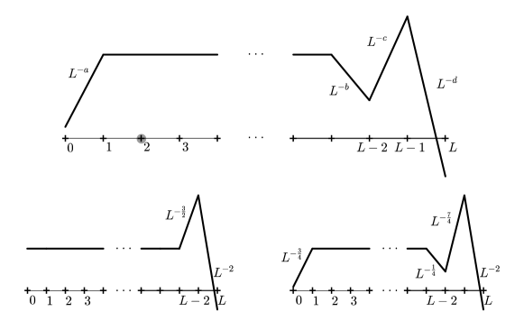
Figure 3: Transition dyagrams for the abc model in the general case and for the choices $(0,0,\frac{3}{2})$ and $(\frac{3}{4},\frac{1}{4},\frac{7}{4})$.

The unique equilibrium measure can be obtained trough reversibility condition:

$$\mu(0) =L^{a}/\mathit{\mathcal{Z}} \mu(x) =1/\mathit{\mathcal{Z}}\;\forall x\in[1,\,L-3]$$ (5.144)

$$\mu(L-2) =L^{b}/\mathit{\mathcal{Z}} \mu(L-1) =L^{b-c}/\mathit{\mathcal{Z}} \mu(L) =L^{2a+3b+c}/\mathit{\mathcal{Z}},$$

where $\mathit{\mathcal{Z}}$ is the normalization factor.

Example 1 ($\mathbf{\frac{5}{8},\frac{1}{4},\frac{7}{4}}$ model )

In this example, for the reference pair $(0,L)$, $Hp.G^{LT}$ holds whereas $Hp.A$ does not.

The state space is $[0,L]$, with all birth and death probabilities equal to $\frac{1}{2}$ except for $P_{0,1}:=\frac{1}{2}L^{-\frac{5}{8}}$, $P_{L-2,L-3}:=\frac{1}{2}L^{-\frac{1}{4}}$, $P_{L-2,L-1}:=\frac{1}{2}L^{-\frac{7}{4}}$ and $P_{L,L-1}:=\frac{1}{2}L^{-\frac{21}{2}}$.

For rigorous computations see the appendix, here we discuss the model at heuristical level.

In view of Markov inequality, in order to check $Hp.G^{LT}$ it is sufficient to show that

$$\sup_{x\in\{1,L-1\}}\frac{{\mathbb{E}}(\tau^{x}_{0,L})}{{\mathbb{E}}(\xi^{0}_{L})}\longrightarrow 0.$$ (5.145)

Since the well in $L-2$ is rather small, the maximum of the mean resistance times can be estimated as the time needed to cross the plateau (of order $L^{2}$):

$$\max_{x\in\{1,L-1\}}\mathbb{E}(\tau_{0,L}^{x})=\mathbb{E}(\tau_{0,L}^{L-2})\asymp L^{2}$$ (5.146)

(see (A.175) for a rigorous computation).

The mean local time can be estimated by using (A.162): the probability that the process starting from $0$ visits $L$ before returning to $0$ can be estimated as the probability of stepping out from $0$ (which is $P_{0,1}=\frac{1}{2}L^{-\frac{5}{8}}$) times the probability of reaching $L-2$ before returning (which is of order $L^{-1})$ times the probability that the process starting from $L-2$ visits $L$ before $0$ (which is of order $L^{\frac{5}{4}}/L^{\frac{7}{4}}$). The mean local time of $0$ (i.e. the time spent in $0$ before the visit to $L$) is therefore

$$\mathbb{E}(\xi_{L}^{0}) = \mathbb{P}\left(\tilde{\tau}_{L}^{0}<\tilde{\tau}_{0}^{0}\right)^{-1}$$ (5.147)

$$= \left(P_{0,1}\mathbb{P}\left(\tilde{\tau}_{L-2}^{1}<\tilde{\tau}_{0}^{1}\right)\mathbb{P}\left(\tilde{\tau}_{L}^{L-2}<\tilde{\tau}_{0}^{L-2}\right)\right)^{-1}\asymp L^{\frac{5}{8}+1+\frac{1}{2}}=L^{\frac{17}{8}}$$

(as proven in (A.162)). Thus, by (5.146), (5.147) the ratio in (5.145) goes like $\asymp L^{-\frac{1}{8}}$ and condition $Hp.G^{LT}$ holds.

On the other hand, the maximum of the mean local time before hitting $0$ or $L$ is reached in $L-2$ and it is of the order of the inverse of $P_{L-2,L-3}$ (i.e. the probability of exiting from $L-2$) times the probabily of exiting the plateau in $0$ (of order $L^{-1})$:

$$\max_{x\in[1,L-1]}\mathbb{E}(\xi_{0,L}^{x})=\mathbb{E}(\xi_{0,L}^{L-2})\asymp\left(P_{L-2,L-3}\mathbb{P}\left(\tilde{\tau}_{0}^{L-3}<\tilde{\tau}_{L-2}^{L-3}\right)\right)\asymp L^{\frac{5}{4}}$$ (5.148)

(see (A.164) for particulars). Thus, by (5.147), (5.148),

$$L\rho_{A}(L)\asymp L\frac{L^{\frac{5}{4}}}{L^{\frac{17}{8}}}=L^{\frac{1}{8}}\longrightarrow\infty$$ (5.149)

that is, condition $A$ does not hold.

Example 2 ($\mathbf{0,0,\frac{3}{2}}$ model )

This choice of parameters corresponds to a birth-and-death chain where all birth and death probabilities are set equal to $\frac{1}{2}$ except for $P_{L-2,L-1}:=\frac{1}{2}L^{-\frac{3}{2}}$ and $P_{L,L-1}:=\frac{1}{2}L^{-3}$.

We show that, for the reference pair $(0,L)$, condition $Hp.B$ holds whereas condition $Hp.G^{LT}$ does not.

Precise computations can be found in the appendix, here we discuss the model at heuristic level.

We start by estimating ${\rho}_{B}(L):=\sup_{z<L}{{\mathbb{E}}({\tau}^{z}_{0,L})/{\mathbb{E}}({\tau}^{0}_{L}})$:

Each time the process is in $L-2$, it has a probability $\frac{1}{2}L^{-\frac{3}{2}}$ of reaching $L$ in two steps, but the probability to find the process in $L-2$ before the transition is of order $L^{-1}$; hence,

$$\mathbb{E}(\tau_{L}^{0})\asymp L\times L^{\frac{3}{2}},$$

see eq. (A.166) for the exact computation.

The maximum of the mean times is dominated by a diffusive contribution:

$$\max_{x\in[1,L-1]}\mathbb{E}(\tau_{0,L}^{x})=\mathbb{E}(\tau_{0,L}^{L-2})\asymp L^{2},$$

as confirmed by (A.175).

Thus, $\rho_{B}\asymp L^{-\frac{1}{2}}$and condition $B$ holds.

Next, we show that

$${\mathbb{P}}\left({\tau}^{L/2}_{\{0,L\}}>{\mathbb{E}}(\xi^{0}_{L})\right)\longrightarrow 1,$$ (5.150)

and, therefore, that $Hp.G^{LT}$ does not hold.

Equation (A.162) allows to compute the mean local time: The probability that the process starting from $0$ visits $L$ before returning to $0$ can be estimated as the probability of reaching $L-2$ before returning (which is of order $L^{-1})$ times the probability that the process starting from $L-2$ visits $L$ before $0$ (which is of order $L/L^{\frac{3}{2}}$). The mean local time of $0$ (i.e. the time spent in $0$ before the visit to $L$) is therefore

$$\mathbb{E}(\xi_{L}^{0})=\mathbb{P}\left(\tilde{\tau}_{L}^{0}<\tilde{\tau}_{0}^{0}\right)^{-1}=\left(\mathbb{P}\left(\tilde{\tau}_{L-2}^{0}<\tilde{\tau}_{0}^{0}\right)\mathbb{P}\left(\tilde{\tau}_{L}^{L-2}<\tilde{\tau}_{0}^{L-2}\right)\right)^{-1}\asymp L^{\frac{3}{2}}$$

(see (A.162) for a rigorous derivation).

Let $M(t):=\max_{s\leq t}\left|\frac{L}{2}-X_{s}^{L/2}\right|$. Since $x=L/2$ is in the middle of the plateau, we can use the diffusive bound $M(t)\asymp\sqrt{t}$ for small $t$. By Markov inequality:

$${\mathbb{P}}\left({\tau}^{L/2}_{\{0,L\}}<L^{\frac{3}{2}}\right)<{\mathbb{P}}\left(M(L^{\frac{3}{2}})>\frac{L}{3}\right)\leq 3\frac{{\mathbb{E}}(M(L^{\frac{3}{2}}))}{L}\asymp L^{-\frac{1}{4}},$$

that implies (5.150).

Appendix A Appendix

A.1 Electric networks

A convenient language to describe the behavior of local and hitting times in the reversible case exploits the analogy with electric networks. Here we recall some useful relation between reversible Markov processes and electric networks. For a more complete discussion, see [DS] and references therein.

We associate with a given reversible Markov chain with transition matrix $P$ a resistance network in the following way:

We call We call “resistance” of an edge $(x,y)$ of the graph associated with the Markov kernel the quantity

$$r_{x,y}:=\left(\mu(x)P_{x,y}\right)^{-1}.$$ (A.151)

Given two disjoint subsets $A,\,B\;\subset\Gamma$, we denote by the capital letter $R_{B}^{A}$ the total resistance between $A$ and $B$, namely, the total electric current that flows in the network if we put all the points in $A$ to the voltage $1$ and all the points in $B$ to the voltage $0$.

It is well-known that the total resistance is related with the mean local time (see def. 2.23) of the Markov chain, i.e. with the Green function, by

$$R_{B}^{x}=\frac{\mathbb{E}(\xi_{B}^{x})}{\mu(x)}.$$ (A.152)

Resistances are reversible objects, i.e. $R_{y}^{x}=R_{x}^{y}.$

The voltage at point $y\in\Gamma$ has a probabilistic interpretation given by

$$V_{B}^{x}(y)=\mathbb{P}\left(\tilde{\tau}_{x}^{y}<\tilde{\tau}_{B}^{y}\right).$$

A.2 h model

A.2.1 Computation of resistances

By reversibility, from (5.141), we easily get

$$\mu(0)=\frac{1}{Z}\qquad\mu(1)=\frac{p^{h}}{Z}\qquad\mu(2)=\frac{p}{Z}\qquad\mu(G)=\frac{p^{-1}}{Z}\qquad$$ (A.153)

Where $Z$ is the renormalization factor. (A.153) can be seen as the Gibbs measure of the system once taken ${\beta}=-\log p$.

By (A.151), (5.141) and (A.153), we get

$$r_{k}:=r_{k,k+1}=\frac{\mathcal{Z}}{2}\times\begin{cases}p^{-h}&\text{ for }k=0\\ p^{-1}&\text{ for }k=1,2\end{cases}$$ (A.154)

A.2.2 Local times

In order to compute $\rho_{A}$, we need to estimate the local time spent in the metastable point $1$ before the transition to $G$ and the maximum among the local times of the points $\left\{0,2\right\}$ before the transition to $1$ or to $G$.

By (A.152), the computation of mean local times is the analogous of the computation of the total resistance of a series of resistances:

$${\mathbb{E}}\left(\xi^{0}_{G}\right) = {\mathbb{E}}\left(\xi^{2}_{1,G}\right)=\mu(0)(r_{0}+r_{1}+r_{2})\asymp p^{-1}$$

$${\mathbb{E}}\left(\xi^{1}_{G}\right) = \mu(1)(r_{1}+r_{2})\asymp p^{-1+h}$$

$${\mathbb{E}}\left(\xi^{2}_{G}\right) = \mu(0)r_{2}\asymp 1$$

$${\mathbb{E}}\left(\xi^{2}_{1,G}\right) = \mu(2)\frac{r_{1}r_{2}}{r_{1}+r_{2}}\asymp 1$$ (A.155)

A.2.3 Hitting times

Obviously,

$${\mathbb{E}}({\tau}{{}^{0}_{1,G}})={\mathbb{E}}(\xi^{0}_{1})\asymp p^{-1+h}$$

$${\mathbb{E}}({\tau}{{}^{2}_{1,G}})={\mathbb{E}}(\xi^{2}_{,G})\asymp 1.$$ (A.156)

More generally, local times provide a useful language to describe the model. E.g. a relation between hitting times and mean times is

$$\mathbb{E}\left(\tau_{A}^{x}\right) =\mathbb{E}\left(\sum_{t=0}^{\tau_{A}^{x}}\ \sum_{y\notin A}1_{X_{t}^{x}=y}\right)$$

$$=\sum_{y\notin A}\mathbb{E}\left(\xi_{A}^{x}(y)\right)=\sum_{y\notin A}\mathbb{E}\left(\xi_{A}^{y}\right)\mathbb{P}\left(\tilde{\tau}_{y}^{x}<\tilde{\tau}_{A}^{x}\right),$$ (A.157)

where we used the strong Markov property at time $\tilde{\tau}_{k}^{0}$ in the last equality. In words, the hitting time is the sum of all local times of the points visited.

Since $\mathbb{P}\left(\tilde{\tau}_{1}^{0}<\tilde{\tau}_{1}^{G}\right)\geq P(1,0)=\frac{1}{2}\asymp 1$, by (A.157), (A.155), we see that

$$\mathbb{E}(\tau_{1}^{G})\asymp\mathbb{E}\left(\xi_{0}^{G}\right)\asymp p^{-1}.$$ (A.158)

A.3 abc model

A.3.1 Computation of resistances

By (A.151), (5.143) and (5.144), we get for $k\in\left\{0,\ldots,L-1\right\}$

$$r_{k}:=r_{k,k+1}=\mathcal{Z}\times\begin{cases}2&\text{ for }k\leq L-3\\ 2L^{c-b}&\text{ for }k>L-3\end{cases}$$ (A.159)

Interesting resistances in our one-dimensional model are the total resistance $R_{0}^{x}$ between $x$ and $0$ and the total resistance $R_{L}^{x}$ between $x$ and $L$.

$$R_{0}^{x}:=\sum_{k=0}^{x-1}r_{k}=\mathcal{Z}\times\begin{cases}2n&\text{ for }x\leq L-2\\ 2(L-2)+2L^{c-b}&\text{ for }x=L-1\end{cases}.$$ (A.160)

$$R_{L}^{x}:=\sum_{k=x}^{L-1}r_{k}=\mathcal{Z}\times\begin{cases}2(L-2-x)+4L^{c-b}&\text{ for }x\leq L-2\\ 2L^{c-b}&\text{ for }x=L-1\end{cases}.$$ (A.161)

A.3.2 Local times

In order to compute $\rho_{A}$, we need to estimate the local time spent in the metastable point $0$ before the transition to $L$ and the maximum among the local times of the points in $\left\{1,\ldots,L-1\right\}$ before the transition to $0$ or to $L$.

By (A.152), the computation of mean local times is the analogous of the computation of the total resistance of a series of resistances. By (A.161) we get

$$\mathbb{E}(\xi_{L}^{0})=\mu(0)R_{L}^{0}=2L^{a}\left((L-2)+2L^{c-b}\right)\asymp L^{a}\left(L+L^{c-b}\right)(1+o(1)).$$ (A.162)

Then, we are interested in the maximum of the local times $\mathbb{E}(\xi_{0,L}^{x})=\mu(x)$$R_{0,L}^{x}$. Depending on the equilibrium measure, we can have the maximum in the plateau $[1,\,L-3]$, in the well $L-2$ or (in principle) in the peak $L-1.$ Since the parallel between two resistances $r$ and $R$, with $r\leq R$ is between $r/2$ and $r$, we get, for the plateau and the well

$$R_{0,L}^{x}=\frac{R_{x}^{0}\left(R_{L}^{0}-R_{x}^{0}\right)}{R_{L}^{0}}\asymp\mathcal{Z}\times\begin{cases}\min\left\{x,\,L+L^{c-b}-x\right\}&\text{ for }x\leq L-2\\ L^{c-b}&\text{ for }x=L-1\end{cases}$$ (A.163)

The maximal local time in the plateau is where the resistance $R_{0,L}^{x}$, the parallel between the resistances $R_{0}^{x}$and $R_{L}^{x}$, is maximal.

• if $1>c-b$, the resistance of the plateau is larger than that of the well and of the peak. Depending on the depth of the well, the maximal resistance is acheived either in the middle of the plateau or in the well. Indeed, an upper bound for $\max_{1\leq x\leq L-3}R_{x,L}^{0}$is obtained by maximizing the r.h.s. of the first equality in (A.163); as a function of $R_{x}^{0}$, this quantity has a maximum for $R_{x}^{0}=R_{L}^{0}/2$; a lower bound for $\max_{1\leq x\leq L-3}R_{x,L}^{0}$is $R_{0,L}^{\lceil L/2\rceil}$. Thus,

  $$\max_{1\leq x\leq L-3}\mathbb{E}(\xi_{0,L}^{x})\asymp L.$$

  The well $x=L-2$ has a large invariant measure that may compensate for the small resistance. Its local time is $\mathbb{E}(\xi_{0,L}^{L-2})=\mu(L-2)\,R_{0,L}^{L-2}\asymp L^{c}$. The local time of the peak $x=L-1$ is always negligible: $\mathbb{E}(\xi_{0,L}^{L-1})=\mu(L-1)R_{0,L}^{L-1}\asymp 1$. Therefore, the maximum local time is either in the middle of the plateau or in the well and

  $$\max_{1\leq x\leq L-1}\mathbb{E}(\xi_{0,L}^{x})\asymp L+L^{c}.$$

• if $1<c-b$, the resistance of the plateau is negligible and the well always wins:

  $$R_{0,L}^{x}\asymp\begin{cases}x&\text{ for }x\leq L-3\\ L^{c-b}&\text{ for }x\geq L-2\end{cases}$$

  Thus,

$$\max_{1\leq x\leq L-3}\mathbb{E}(\xi_{0,L}^{x})\asymp\mu(L-2)R_{0,L}^{L-2}.$$

Altogether,

$$\max_{x\leq L-1}\mathbb{E}(\xi_{0,L}^{x})=\max_{x\leq L-1}\mu(x)\,R_{0,L}^{x}\asymp\begin{cases}\mathbb{E}(\xi_{0,L}^{\lceil\frac{L}{2}\rceil})\asymp L&\text{ for }c<1\\ \mathbb{E}(\xi_{0,L}^{L-2})\asymp L^{c}&\text{ for }1\leq c\leq b+1\\ \mathbb{E}(\xi_{0,L}^{L-2})\asymp L^{b+1}&\text{ for }c>b+1\end{cases}.$$ (A.164)

A.3.3 Hitting times

In the one-dimensional case, $\mathbb{P}\left(\tilde{\tau}_{k}^{0}<\tilde{\tau}_{L}^{0}\right)=1$ for all $k\in[1,L-1]$. By (A.157), (A.159), we see that

$$\mathbb{E}(\tau_{L}^{0})=\sum_{k=0}^{L-1}\mathbb{E}\left(\xi_{L}^{k}\right)\mathbb{P}\left(\tilde{\tau}_{k}^{0}<\tilde{\tau}_{L}^{0}\right)=\sum_{k=0}^{L-1}\mu(k)R_{L}^{k}$$

$$\mathbb{=E}(\xi_{L}^{0})+\sum_{k=1}^{L-3}\left(2(L-2-k)+2L^{c-b}\right)+\pi(L-2)4L^{c-b}+\pi(L-1)2L^{c-b}$$ (A.165)

by (LABEL:eq:LT), (5.144)

$$\mathbb{E}(\tau_{L}^{0})\asymp \left(L^{a}\left(L+L^{c-b}\right)+L^{2}+L^{c-b+1}+L^{c}+1\right)(1+o(1))=$$

$$\left(L^{a}+L\right)\left(L^{c-b}+L\right)(1+o(1)),$$ (A.166)

where we used $a>b.$

The computation of $\mathbb{E}(\tau_{0,L}^{x})$ is slightly more intricate:

In one dimension, $\mathbb{P}\left(\tilde{\tau}_{k}^{x}<\tilde{\tau}_{0,L}^{x}\right)$ is equal to $\mathbb{P}\left(\tilde{\tau}_{k}^{x}<\tilde{\tau}_{L}^{x}\right)$ if $k\leq x$ and to $\mathbb{P}\left(\tilde{\tau}_{k}^{x}<\tilde{\tau}_{0}^{x}\right)$ if $k>x$.

$$\mathbb{P}\left(\tilde{\tau}_{k}^{x}<\tilde{\tau}_{0,L}^{x}\right)=\begin{cases}\mathbb{P}\left(\tilde{\tau}_{k}^{x}<\tilde{\tau}_{L}^{x}\right)=\frac{R_{L}^{k}}{R_{L}^{x}}&\text{ if }k\leq x\\ \mathbb{P}\left(\tilde{\tau}_{k}^{x}<\tilde{\tau}_{L}^{x}\right)=\frac{R_{0}^{k}}{R_{L}^{x}}&\text{ if }k>x\end{cases}$$

By (A.157), for $x\in[1,\,L-1]$,

$$\mathbb{E}(\tau_{0,L}^{x}) = \sum_{k=1}^{x-1}\mathbb{E}(\xi_{0,L}^{k})\mathbb{P}\left(\tilde{\tau}_{k}^{x}<\tilde{\tau}_{L}^{x}\right)+\mathbb{E}(\xi_{0,L}^{x})+\sum_{k=x+1}^{L-1}\mathbb{E}(\xi_{0,L}^{k})\mathbb{P}\left(\tilde{\tau}_{k}^{x}<\tilde{\tau}_{0}^{x}\right)$$ (A.167)

$$= \displaystyle\frac{R^{x}_{L}\sum_{k=1}^{x-1}\mu(k)R^{k}_{0}+\mu(x)R^{0}_{x}R^{x}_{L}+R^{0}_{x}\sum_{k=x+1}^{L-1}\mu(k)R^{k}_{L}}{R^{0}_{L}}$$

• Let us consider first the plateau $x\leq L-3.$ By (A.160)

  $$\sum_{k=1}^{x-1}\mu(k)R^{k}_{0}\asymp x^{2},$$ (A.168)

  and by (A.161)

  $$\sum_{k=x+1}^{L-1}\mu(k)R^{k}_{L} = \sum_{k=x+1}^{L-3}\left(2(L-2-k)+4L^{c-b}\right)+2L^{c}+2$$ (A.169)

  $$\asymp (L-x)^{2}+L^{c-b+1}+L^{c}.$$

  Plugging (A.160,A.161,A.168,A.169) into (A.167), we get

  $$\mathbb{E}(\tau_{0,L}^{x})\asymp x\frac{\left(L-x+L^{c-b}\right)x++(L-x)^{2}+L^{c-b+1}}{L+L^{c-b}},$$ (A.170)

  where we used $\mu(L-2)R_{L}^{L-2}\asymp L^{b}L^{c-b}$. A little algebra shows that

  $$\mathbb{E}(\tau_{0,L}^{x})\asymp xL-\frac{L^{c-b}-L}{L^{c-b}+L}x^{2}\asymp\begin{cases}xL-x^{2}&\text{ for }1\geq c-b\\ xL+x^{2}&\text{ for }1<c-b\end{cases}$$

  In both cases,

  $$\max_{1\leq x\leq L-3}\mathbb{E}(\tau_{0,L}^{x})\asymp L^{2}$$

• if $x=L-2$, the three terms in the numerator of l.s.h. of (A.167) become:

  $$R^{L-2}_{L}\sum_{k=1}^{L-3}\mu(k)R^{k}_{0}\asymp\mathcal{Z}L^{2+c-b}$$ (A.171)

  $$\mu(L-2)R^{0}_{L-2}R^{L-2}_{L}\asymp\mathcal{Z}L^{b}LL^{c-b}=\mathcal{Z}L^{c+1}$$ (A.172)

  $$R^{0}_{L-2}\mu(L-1)R^{L-1}_{L}\asymp\mathcal{Z}L^{b-c}LL^{c-b}=\mathcal{Z}L,$$ (A.173)

  where we used A.161.

  By using (A.167) and A.161, we estimate

  $$\mathbb{E}(\tau_{0,L}^{L-2})\asymp \frac{L^{c-b+2}+L^{c+1}}{L^{c-b}+L}x^{2}\asymp\begin{cases}L^{c-b+1}+L^{c}&\text{ for }1\geq c-b\\ L^{2}+L^{b+1}&\text{ for }1<c-b\end{cases}$$ (A.174)

• if $x=L-1$, it is easy to see that

  $$\mathbb{E}(\tau_{0,L}^{L-1})\leq\mathbb{E}(\tau_{0,L}^{L-2}).$$

Putting together the three cases, we get

$$\max_{x\in\{1,L-1\}}\mathbb{E}(\tau_{0,L}^{x})\asymp\begin{cases}L^{b+1}&\text{ for }b>1\text{ and }c>b+1\\ L^{2}&\text{ otherwise. }\end{cases}$$ (A.175)

References

- [1] D. Aldous, “Markov chains with almost exponential hitting times” Sto.Proc.Appl 13, 305–310 (1982).
- [2] D. Aldous, M. Brown, “Inequalities for rare events in time reversible Markov chains I”, in Stochastic Inequalities, M. Shaked and Y.L. Tong eds., pp. 1–16, Lecture Notes of the Institute of Mathematical Statistics, vol. 22 (1992).
- [3] D. Aldous, M. Brown, “ Inequalities for rare events in time reversible Markov chains II”, Sto.Proc.Appl 44, 15-25 (1993).
- [4] G. Ben Arous, R. Cerf, “Metastability of the three-dimensional Ising model on a torus at very low temperature”, Electron. J Probab. 1, 10 (1996).
- [5] J. Beltran, C. Landim, “Tunneling and metastability of continuous time Markov chains”, J. Stat. Phys. 140 no. 6, 1065–1114 (2010).
- [6] A. Bianchi, A. Gaudilliere, “Metastable states, quasi-stationary and soft masures, mixing time asymptotics via variational principles”, arXiv:1103.1143, (2011).
- [7] O. Benois, C. Landim, C. Mourragui, “Hitting Times of Rare Events in Markov Chains”, J. Stat. Phys. 153, 967–990 (2013).
- [8] S. Bigelis, E.N.M. Cirillo, J.L. Lebowitz, and E.R. Speer, “Critical droplets in metastable probabilistic cellular automata”, Phys. Rev. E 59, 3935 (1999).
- [9] A. Bovier, “Metastability: a potential-theoretic approach”, In International Congress of Mathematicians, vol. III, pp. 499–518, Eur. Math. Soc., Zürich (2006).
- [10] A. Bovier, M. Eckhoff, V. Gayrard, and M. Klein, “Metastability and small eigenvalues in Markov chains”, J. Phys. A 33(46), L447–L451 (2000).
- [11] A. Bovier, M. Eckhoff, V. Gayrard, M. Klein, “Metastability in stochastic dynamics of disordered mean-field models”, Probab. Theory Related Fields 119(1), 99–161 (2001).
- [12] A. Bovier, M. Eckhoff, V. Gayrard, M. Klein, “Metastability and low lying spectra in reversible Markov chains”, Comm. Math. Phys. 228, 219–255 (2002).
- [13] A. Bovier, M. Eckhoff, V. Gayrard, M. Klein, “Metastability in reversible diffusion processes. I. Sharp asymptotics for capacities and exit times”, J. Eur. Math. Soc. (JEMS) 6(4), 399–424 (2004).
- [14] A. Bovier, F. den Hollander, F.R. Nardi, “Sharp asymptotics for Kawasaki dynamics on a finite box with open boundary”, Probability Theory and Related Fields 135, 265–310 (2006).
- [15] A. Bovier, F. den Hollander, C. Spitoni, “Homogeneous nucleation for Glauber and Kawasaki dynamics in large volumes at low temperature”, Ann. Probab. 38, (2010).
- [16] A. Bovier, F. Manzo, “Metastability in Glauber dynamics in the low temperature limit: beyond exponential asymptotic”, Journ. Stat. Phys. 107, 757–779 (2002).
- [17] M. Brown, “Consequences of monotonicity for Markov transition functions”, City College, CUNY report MB89-03 (1990).
- [18] M. Brown, “Error bounds for exponential approximations of geometric convolution”, Ann. Probab. 18 , 1388-1402 (1990).
- [19] M. Brown, “Interlacing eigenvalues in time reversible Markov chains”, Math. Oper. Res.24 , 847-864 (1999).
- [20] M. Cassandro, A. Galves, E. Olivieri, and M.E. Vares, “Metastable behavior of stochastic dynamics: A pathwise approach.”, Journ. Stat. Phys. 35, 603–634 (1984).
- [21] O. Catoni, R. Cerf, “The exit path of a Markov chain with rare transitions”, ESAIM Probab. Statist. 1, 95–144 (1995/97).
- [22] O. Catoni, “Simulated annealing algorithms and Markov chains with rare transitions”, Séminaire de Probabilités, XXXIII 1709, 69–119 (1999).
- [23] O. Catoni, A. Trouvé, “Parallel annealing by multiple trials: a mathematical study.” Simulated annealing 129–143, Wiley-Intersci. Ser. Discrete Math., (1992).
- [24] R. Cerf, F. Manzo, “Nucleation and growth for the Ising model in d dimensions at very low temperatures” Ann. of Prob. 41, 3697–3785 (2013).
- [25] E.N.M. Cirillo, J.L. Lebowitz, “Metastability in the two-dimensional Ising model with free boundary conditions”, Journ. Stat. Phys. 90, 211–226 (1998).
- [26] E.N.M. Cirillo and F.R. Nardi, “Metastability for a stochastic dynamics with a parallel heath bath updating rule”, Journ. Stat. Phys. 110, 183–217 (2003).
- [27] Cirillo E.N.M. and F.R. Nardi, “Relaxation height in energy landscapes: an application to multiple metastable states”, Journ. Stat. Phys., 150, 1080-1114, (2013).
- [28] E.N.M. Cirillo, F.R. Nardi, and C. Spitoni, “Metastability for reversible probabilistic cellular automata with self-interaction”, Journ. Stat. Phys. 132, 431–471 (2008).
- [29] E.N.M. Cirillo, E. Olivieri, “ Metastability and nucleation for the Blume-Capel model: different mechanisms of transition.”, Journ. Stat. Phys. 83, 473–554 (1996).
- [30] Dehghanpour P., R. Schonmann, “ A nucleation and growth model”, Probab. Theory Relat. Fields, 107, 123–135, (1997).
- [31] P. Dehghanpour, R. Schonmann, “ Metropolis dynamics relaxation via nucleation and growth”, Commun. Math. Phys. 188, 89–119 (1997).
- [32] R. Fernández, F. Manzo, F.R. Nardi, E. Scoppola, J. Sohier, “title” work in progress.
- [33] J.A. Fill, V. Lyzinski, “Hitting times and interlacing eigenvalues: a stochastic appoach using intertwining”, Journal of Theoretical Probability, bf 28, Springer Science+Business Media New York 201210.1007/s10959-012-0457-9 (2012).
- [34] M.I. Freidlin, A.D. Wentzell, “Random perturbations of dynamical systems”, Grundlehren der Mathematischen Wissenschaften [Fundamental Principles of Mathematical Sciences], vol. 260. Springer–Verlag, New York (1984).
- [35] A. Gaudillière, W.Th.F. den Hollander, F.R. Nardi, E. Olivieri, and E. Scoppola, “Ideal gas approximation for a two–dimensional rarefied gas under Kawasaki dynamics”, Stochastic Processes and their Applications 119, 737–774 (2009).
- [36] A. Gaudillière and F.R. Nardi, “An upper bound for front propagation velocities inside moving populations”, online on the website and in printing on Brazilian Journal of Probability and Statistics 24, 256–278 (2010).
- [37] A. Gaudillière, E. Olivieri, E. Scoppola, “Nucleation pattern at low temperature for local kawasaki dynamics in two-dimensions”, Markov Processes Relat. Fields, 11, 553-628, (2005).
- [38] F. den Hollander, F.R. Nardi, E. Olivieri, E. Scoppola, “Droplet growth for three-dimensional Kawasaki dynamics”, Probability Theory and Related Fields 125, 153–194 (2003).
- [39] F. den Hollander, F.R. Nardi, and A. Troiani, “Metastability for low – temperature Kawasaki dynamics with two types of particles”, Electronic Journ. of Probability 17, 1-26 (2012).
- [40] F. den Hollander, F.R. Nardi, and A. Troiani, “Kawasaki dynamics with two types of particles: stable/metastable configurations and communication heights”, Journ. Stat. Phys. 145(6), 1423–1457 (2011).
- [41] F. den Hollander, F.R. Nardi, and A. Troiani, “Kawasaki dynamics with two types of particles : critical droplets.”, Journ. Stat. Phys. 149(6), 1013–1057 (2012).
- [42] F. den Hollander, E. Olivieri, and E. Scoppola, “Metastability and nucleation for conservative dynamics”, J. Math. Phys. 41, 1424–1498 (2000).
- [43] J. Keilson, Markov Chain Models–Rarity and Exponentiality, Springer-Verlag (1979).
- [44] Kotecky R. E. Olivieri, “Droplet Dynamics for asymmetric Ising model”, Journ. Stat. Phys., 70, 1121-1148, (1993).
- [45] R. Kotecky, E. Olivieri, “Shapes of growing droplets - a model of escape from the metastable phase”, Journ. Stat. Phys. 75, 409-506 (1994).
- [46] F. Manzo, F.R. Nardi, E. Olivieri, and E. Scoppola, “On the essential features of metastability: tunnelling time and critical configurations”, Journ. Stat. Phys. 115, 591–642 (2004).
- [47] F. Manzo E. Olivieri, “Relaxation patterns for competing metastable states a nucleation and growth model”, Markov Process. Relat. Fields 4, 549–570 (1998).
- [48] F. Manzo, E. Olivieri, “Dynamical Blume-Capel model: competing metastable states at infinite volume”, Journ. Stat. Phys. 115, 591–641 (2001).
- [49] F.R. Nardi and E. Olivieri, “Low temperature stochastic dynamics for an Ising model with alternating field”, Markov Processes fields 2, 117–166 (1996).
- [50] F.R. Nardi, E. Olivieri, and E. Scoppola, “Anisotropy effects in nucleation for conservative dynamics”, Journ. Stat. Phys. 119, 539–595 (2005).
- [51] F.R. Nardi and C. Spitoni, “Sharp Asymptotics for Stochastic Dynamics with Parallel Updating Rule with self-interaction”, Journal of Statistical Physics 146, 701–718 (2012).
- [52] E.J. Neves and R.H. Schonmann, “Critical droplets and metastability for a GLauber dynamics at very low temperature”, Comm. Math. Phys. 137, 209–230 (1991).
- [53] E.J. Neves and R.H. Schonmann, “Behavior of droplets for a class of Glauber dynamics at very low temperature”, Probab. Theory Related Fields 91(3-4), 331–354 (1992)
- [54] E. Olivieri and E. Scoppola, “Markov chains with exponentially small transition probabilities: First exit problem from general domain I. The reversible case”, Journ. Stat. Phys. 79, 613–647 (1995).
- [55] E. Olivieri and E. Scoppola, “Markov chains with exponentially small transition probabilities: First exit problem from general domain II. The general case”, Journ. Stat. Phys. 84, 987–1041 (1996).
- [56] E. Olivieri and M.E. Vares, “Large deviations and metastability”. Encyclopedia of Mathematics and its Applications, 100. Cambridge University Press, Cambridge, (2005).
- [57] R.H. Schonmann, “The pattern of escape from metastability of a stochastic Ising model phase coexistence region”, Commun. Math. Phys. 147, 231–240 (1992).
- [58] R.H. Schonmann, “Slow droplets driven relaxation of stochastic Ising models in the vicinity of phase coexistence region”, Commun. Math. Phys. 161, 1–49 (1994).
- [59] R.H. Schonmann and S. Shlosman, “Wulff droplets and metastable relaxation of Kinetic Ising models”, Commun. Math. Phys. 194, 389–462 (1998).
- [60] E. Scoppola, “Renormalization group for Markov chains and application to metastability”. J. Statist. Phys. vol. 73, pp. 83–121, (1993).
- [61] E. Scoppola, “Metastability for Markov chains: a general procedure based on renormalization group ideas”, Probability and phase transition (Cambridge, 1993), NATO Adv. Sci. Inst. Ser. C Math. Phys. Sci., vol. 420, pp. 303–322, (1994).
- [62] A. Trouvé, “Partially parallel simulated annealing: low and high temperature approach of the invariant measure”, Applied stochastic analysis (New Brunswick, NJ, 1991), 262–278, Lecture Notes in Control and Inform. Sci. 177, Springer, Berlin, (1992).
- [63] , A. Trouvé, ”Rough Large Deviation Estimates for the Optimal Convergence Speed Exponent of Generalized Simulated Annealing Algorithms” Ann. Inst. H. Poincare Prob. Stat. 32, 299–348 (1994)