PlanIt: A Crowdsourcing Approach for Learning to Plan Paths
from Large Scale Preference Feedback

Abstract

We consider the problem of learning user preferences over robot trajectories for environments rich in objects and humans. This is challenging because the criterion defining a good trajectory varies with users, tasks and interactions in the environment. We represent trajectory preferences using a cost function that the robot learns and uses it to generate good trajectories in new environments. We design a crowdsourcing system - PlanIt, where non-expert users label segments of the robot’s trajectory. PlanIt allows us to collect a large amount of user feedback, and using the weak and noisy labels from PlanIt we learn the parameters of our model. We test our approach on 122 different environments for robotic navigation and manipulation tasks. Our extensive experiments show that the learned cost function generates preferred trajectories in human environments. Our crowdsourcing system is publicly available for the visualization of the learned costs and for providing preference feedback: http://planit.cs.cornell.edu

I Introduction

One key problem robots face in performing tasks in human environments is identifying trajectories desirable to the users. In this work we present a crowdsourcing system PlanIt that learns user preferences by taking their feedback over the Internet. In previous works, user preferences are usually encoded as a cost over trajectories, and then optimized using planners such as RRT* [1], CHOMP [2], TrajOpt [3]. However, most of these works optimize expert-designed cost functions based on different geometric and safety criteria [4, 5, 6]. While satisfying safety criteria is necessary, they alone ignore the contextual interactions in human environments [7]. We take a data driven approach and learn a context-rich cost over the trajectories from the preferences shown by non-expert users.

Figure 1: Various human activities with the objects in the environment affect how a robot should navigate in the environment. The figure shows an environment with multiple human activities: (1) two humans interacting, (2) watching, (3) walking, (4) working, (5) sitting, and (6) reaching for a lamp. We learn a spatial distribution for each activity, and use it to build a cost map (aka planning affordance map) for the complete environment. Using the cost map, the robot plans a preferred trajectory in the environment.

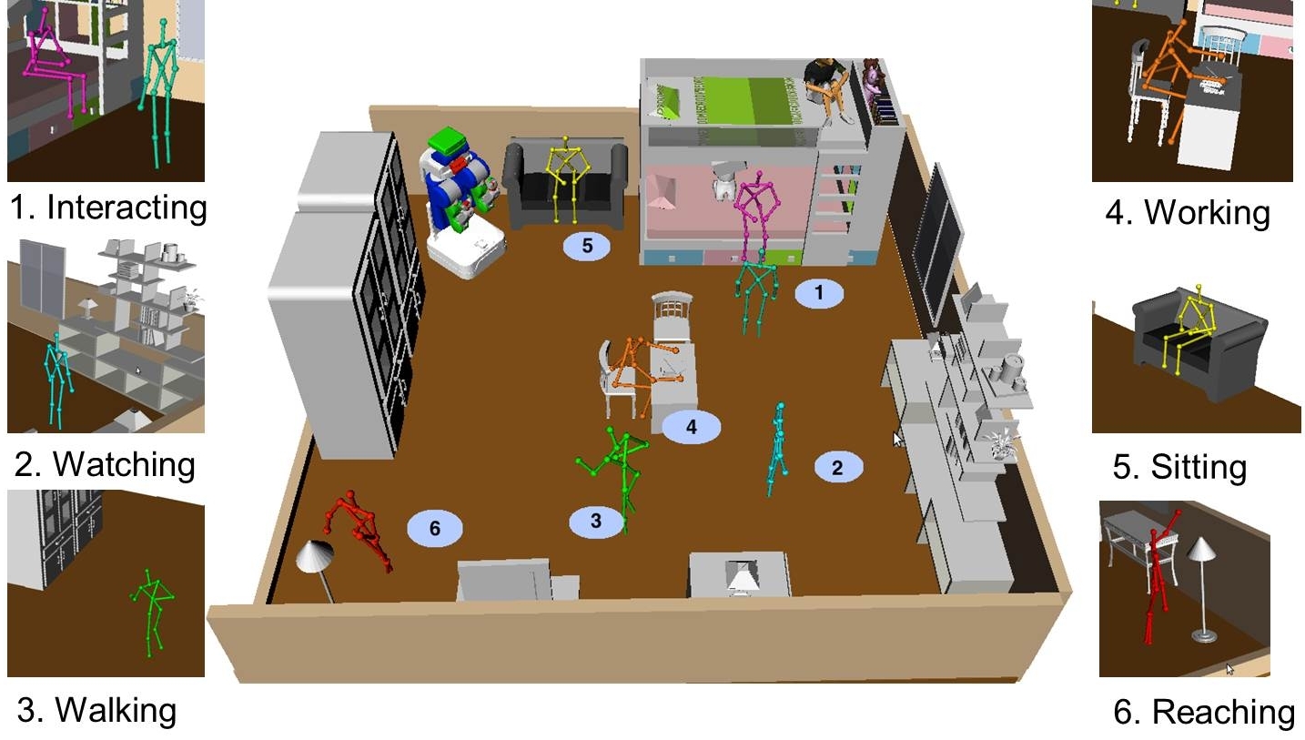
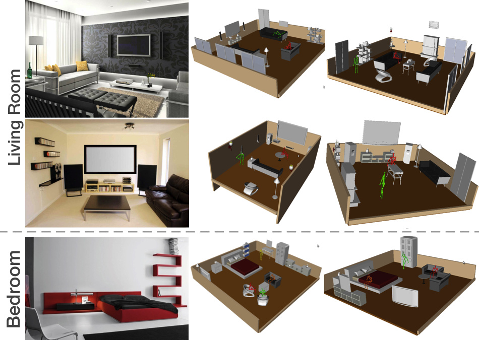
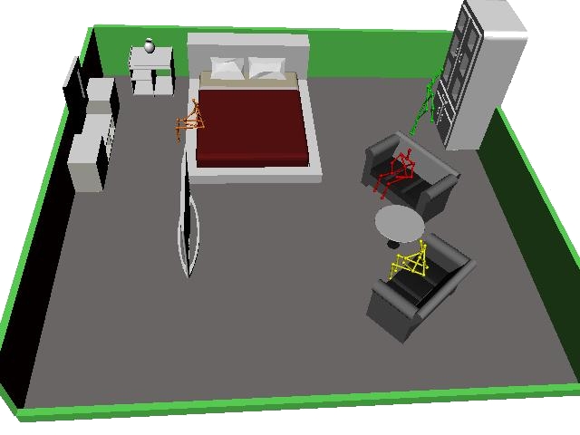
In this work we model user preferences arising during human activities. Humans constantly engage in activities with their surroundings – watching TV or listening to music, etc. – during which they prefer minimal interruption from external agents that share their environment. For example, a robot that blocks the view of a human watching TV is not a desirable social agent. How can a robot learn such preferences and context? This problem is further challenging because human environments are unstructured, and as shown in Fig. 1 an environment can have multiple human activities happening simultaneously. Therefore generalizing the learned model to new environments is a key challenge.

We formulate the problem as learning to ground each human activity to a spatial distribution signifying regions crucial to the activity. We refer to these spatial distributions as planning affordances and parameterize the cost function using these distributions. Our affordance representation is different by relating to the object’s functionality, unlike previous works which have an object centric view. The commonly studied discrete representation of affordances [9, 10, 11, 12] are of limited use in planning trajectories. For example, a TV has a watchable affordance and undergoes a watching activity, however these labels themselves are not informative enough to convey to the robot that it should not move between the user and the TV. The grounded representation we propose in this work is more useful for planning tasks than the discrete representations.

To generalize well across diverse environments we develop a crowdsourcing web-service PlanIt to collect large-scale preference data. On PlanIt we show short videos (mostly $<$ 15 sec) to non-expert users of the robot navigating in context-rich environments with humans performing activities. As feedback users label segments of the videos as good, bad or neutral. While previous methods of eliciting feedback required expensive expert demonstrations in limited environments, PlanIt is usable by non-expert users and scales to a large number of environments. This simplicity comes at the cost of weak and noisy feedback. We present a generative model of the preference data obtained.

We evaluate our approach on a total of 122 bedroom and living room environments. We use OpenRave [13] to generate trajectories in these environments and upload them to PlanIt database for user feedback. We quantitatively evaluate our learned model and compare it to previous works on human-aware planning. Further, we validate our model on the PR2 robot to navigate in human environments. The results show that our learned model generalizes well to the environments not seen before.

In the following sections, we formally state the planning problem, give an overview of the PlanIt engine in Section IV, discuss the cost parametrization through affordance in Section V-A, describe the learning algorithm in Section V-B, and show the experimental evaluation in Section VI.

II Related Work

Learning from demonstration (LfD). One approach to learning preferences is to mimic an expert’s demonstrations. Several works have built on this idea such as the autonomous helicopter flights [14], the ball-in-a-cup experiment [15], planning 2-D paths [16], etc. These approaches are applicable in our setting. However, they are expensive in that they require an expert to demonstrate the optimal trajectory. Such demonstrations are difficult to elicit on a large scale and over many environments. Instead we learn with preference data from non-expert users across a wide variety of environments.

Planning from a cost function. In many applications, the goal is to find a trajectory that optimizes a cost function. Several works build upon the sampling based planner RRT [17, 1] to optimize various cost heuristics [18, 19]. Some approaches introduce sampling bias [20] to guide the planner. Alternative approaches include recent trajectory optimizers CHOMP [2] and TrajOpt [3]. We are complementary to these works in that we learn a cost function while the above approaches optimize cost functions.

Modeling human motion for navigation path. Sharing environment with humans requires robots to model and predict human navigation patterns and generate socially compliant paths [21, 22, 23]. Recent works [24, 25, 26] model human motion to anticipate their actions for better human-robot collaboration. Instead we model the spatial distribution of human activities and the preferences associated with those activities.

Affordances in robotics. Many works in robotics have studied affordances. Most of the works study affordance as cause-effect relations, i.e. the effects of robot’s actions on objects [9, 27, 28, 10]. We differ from these works in the representation of affordance and in its application to planning user preferred trajectories. Further, we consider context-rich environments where humans interact with various objects, while such context was not important to previous works. Similar to Jiang et al. [29], our affordances are also distributions, but they used them for scene arrangement while we use them for planning.

User preferences in path planning. User preferences have been studied in human-robot interaction literature. Sisbot et al. [4, 30] and Mainprice et al. [6] planned trajectories satisfying user specified preferences such as the distance of the robot from humans, visibility of the robot and human arm comfort. Dragan et al. [31] used functional gradients [2] to optimize for legibility of robot trajectories. We differ from these in that we learn the cost function capturing preferences arising during human-object interactions. Jain et al. [32, 7] learned a context-rich cost via iterative feedback from non-expert users. Similarly, we also learn from the preference data of non-expert users. However, we use crowdsourcing like Chung et al. [33] for eliciting user feedback which allows us to learn from large amount of preference data. In experiments, we compare against Jain’s trajectory preference perceptron algorithm.

III Context-aware planning problem

Figure 2: Preference-based Cost calculation of a trajectory. The trajectory $\mathcal{T}_{A}$ is preferred over $\mathcal{T}_{B}$ because it does not interfere with the human activities. The cost of a trajectory decomposes over the waypoints $t_{i}$, and the cost depends on the location of the objects and humans associated with an activity.

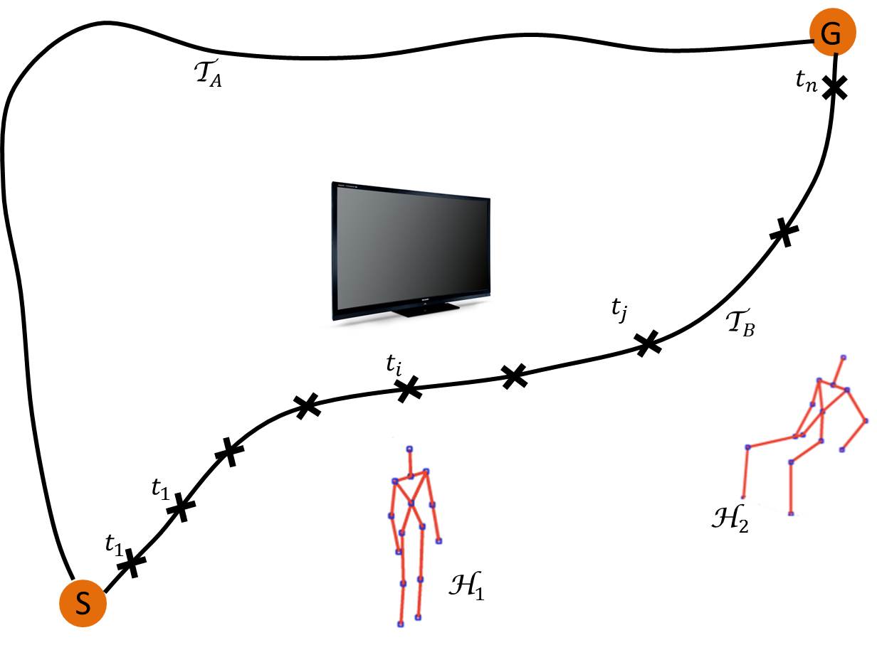
The planning problem we address is: given a goal configuration $G$ and a context-rich environment $E$ (containing objects, humans and activities), the algorithm should output a desirable trajectory $\hat{\mathcal{T}}$. We consider navigation trajectories and represent them as a sequence of discrete 2D waypoints, i.e., $\mathcal{T}=\{t_{1},\ldots,t_{n}\}$. Our model is easily extendable to higher dimensional manipulation trajectories, we demonstrate this in Section VI-G.

In order to encode the user’s desirability we use a positive cost function $\mathbf{\Psi}(\cdot)$ that maps trajectories to a scalar value. Trajectories with lower cost indicate greater desirability. We denote the cost of trajectory $\mathcal{T}$ in environment $E$ as $\mathbf{\Psi}(\mathcal{T}|E)$ where $\mathbf{\Psi}$ is defined as:

$$\mathbf{\Psi}|E:\mathcal{T}\longrightarrow\mathbb{R}$$

The context-rich environment $E$ comprises humans, objects and activities. Specifically, it models the human-human and human-object interactions. The robot’s goal is to learn the spatial distribution of these interactions in order to plan good trajectories that minimally interrupt human activities. The key challenge here lies in designing an expressive cost function that accurately reflects user preferences, captures the rich environment context, and can be learned from data.

Fig. 2 illustrates how the cost of a trajectory is the cumulative effect of the environment at each waypoint. We thus define a trajectory’s cost as a product of the costs over each waypoint:

$$\mathbf{\Psi}(\mathcal{T}=\{t_{1},..,t_{n}\}|E)=\prod_{i}\Psi_{a_{i}}(t_{i}|E)\,\,$$ (1)

In the above equation, $\Psi_{a_{i}}(t_{i}|E)$ is the cost of waypoint $t_{i}$ and its always positive. Because user preferences vary over activities, we learn a separate cost for each activity. $\Psi_{a}(\cdot)$ denotes the cost associated with an activity $a\in E$. The robot navigating along a trajectory often interferes with multiple human activities e.g., trajectory $\mathcal{T}_{\mathcal{B}}$ in Fig. 2. Thus we associate with each waypoint $t_{i}$ an activity $a_{i}$ it interacts with, as illustrated in Eq. (1).

Figure 3: An illustration of our PlanIt system. Our learning system has three main components (i) cost parameterization through affordance; (ii) The PlanIt engine for receiving user preference feedback; and (iii) Learning algorithm. (Best viewed in color)

The cost function changes with the activities happening in the environment. As illustrated in Fig. 2, the robot prefers the trajectory $\mathcal{T}_{A}$ over the otherwise preferred shorter trajectory $\mathcal{T}_{B}$ because the latter interferes with human interactions (e.g., $H_{2}$ is watching TV).

IV PlanIt: A crowdsourcing engine

Rich data along with principled learning algorithms have achieved much success in robotics problems such as grasping [34, 35, 36], manipulation [37], trajectory modeling [38] etc. Inspired by such previous works, we design PlanIt: a scalable approach for learning user preferences over robot trajectories across a wide-variety of environments: http://planit.cs.cornell.edu

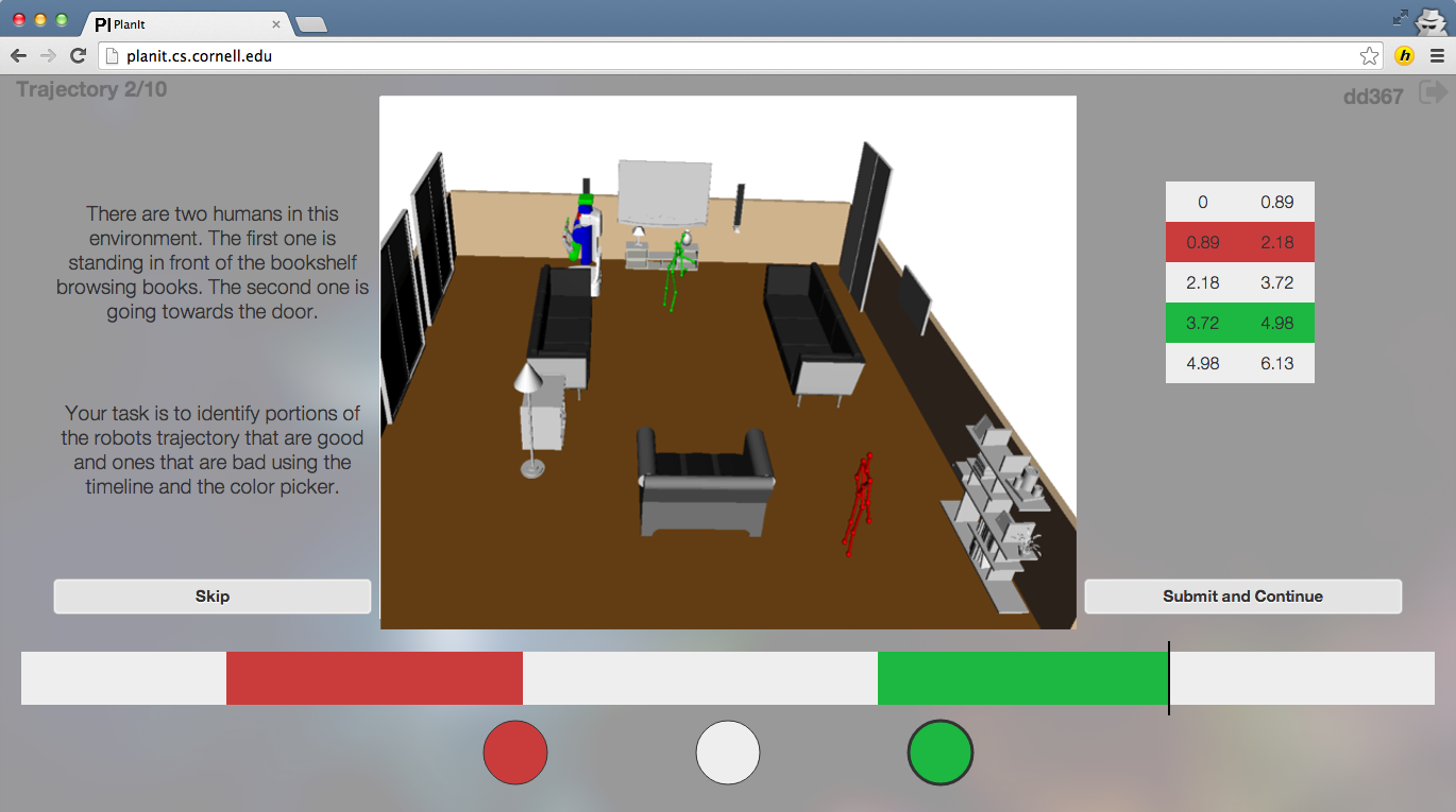
On PlanIt’s webpage users watch videos of robot navigating in contextually-rich environments and reveal their preferences by labeling video segments (Fig. 4). We keep the process simple for users by providing three label choices {bad, neutral, good}. For example, the trajectory segments where the robot passes between a human and TV can be labeled as bad, and segments where it navigates in open space as neutral. We now discuss three aspects of PlanIt.

A. Weak labels from PlanIt: In PlanIt’s feedback process, users only label parts of a trajectory (i.e. sub-trajectory) as good, bad or neutral. For the ease of usability and to reduce the labeling effort, users only provide the labels and do not reveal the (latent) reason for the labels. We capture the user’s intention as a latent variable in the learning algorithm (discussed in Section V-B).

The user feedback in PlanIt is in contrast to other learning-based approaches such as learning from the expert’s demonstrations (LfD) [14, 15, 16, 39] or the co-active feedback [32, 7]. In both LfD and co-active learning approaches it is time consuming and expensive to collect the preference data on a robotic platform and across many environments. Hence these approaches learn using limited preference data from users. On the other hand, PlanIt’s main objective is to leverage the crowd and learn from the non-expert users across a large number of environments.

B. Generating robot trajectory videos: We sample many trajectories (using RRT [17]) for the PR2 robot in human environments using OpenRAVE [13]. We video record these trajectories and add them to PlanIt’s trajectory database. The users watch the short videos of the PR2 interacting with human activities, and reveal their preferences. We also ensure that trajectories in the database are diverse by following the ideas presented in [40, 32]. As of now the PlantIt’s database has 2500 trajectories over 122 environments. In Section VI we describe the data set.

Figure 4: PlanIt Interface. Screenshot of the PlanIt video labeling interface. The video shows a human walking towards the door while other human is browsing books, with text describing the environment on left. As feedback the user labels the time interval where the robot crosses the human browsing books as red, and the interval where the robot carefully avoids the walking human as green. (Best viewed in color)

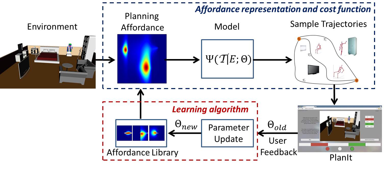
C. Learning system: In our learning system, illustrated in Fig. 3, the learned model improves as more preference data from users become available. We maintain an affordance library with spatial distributions for each human activity. When the robot observes an environment, it uses the distributions from the library and builds a planning affordance map (aka cost function) for the environment. The robot then samples trajectories from the cost function and presents them on the PlanIt engine for feedback.

V Learning Algorithm

We first discuss our parameterization of the cost function and then the procedure for learning the model parameters.

V-A Cost Parameterization through Affordance

In order to plan trajectories in human environments we model the human-object relationships. These relationships are called ‘object affordances’. In this work we model the affordances such that they are relevant to path planning and we refer to them as ‘planning affordances’.

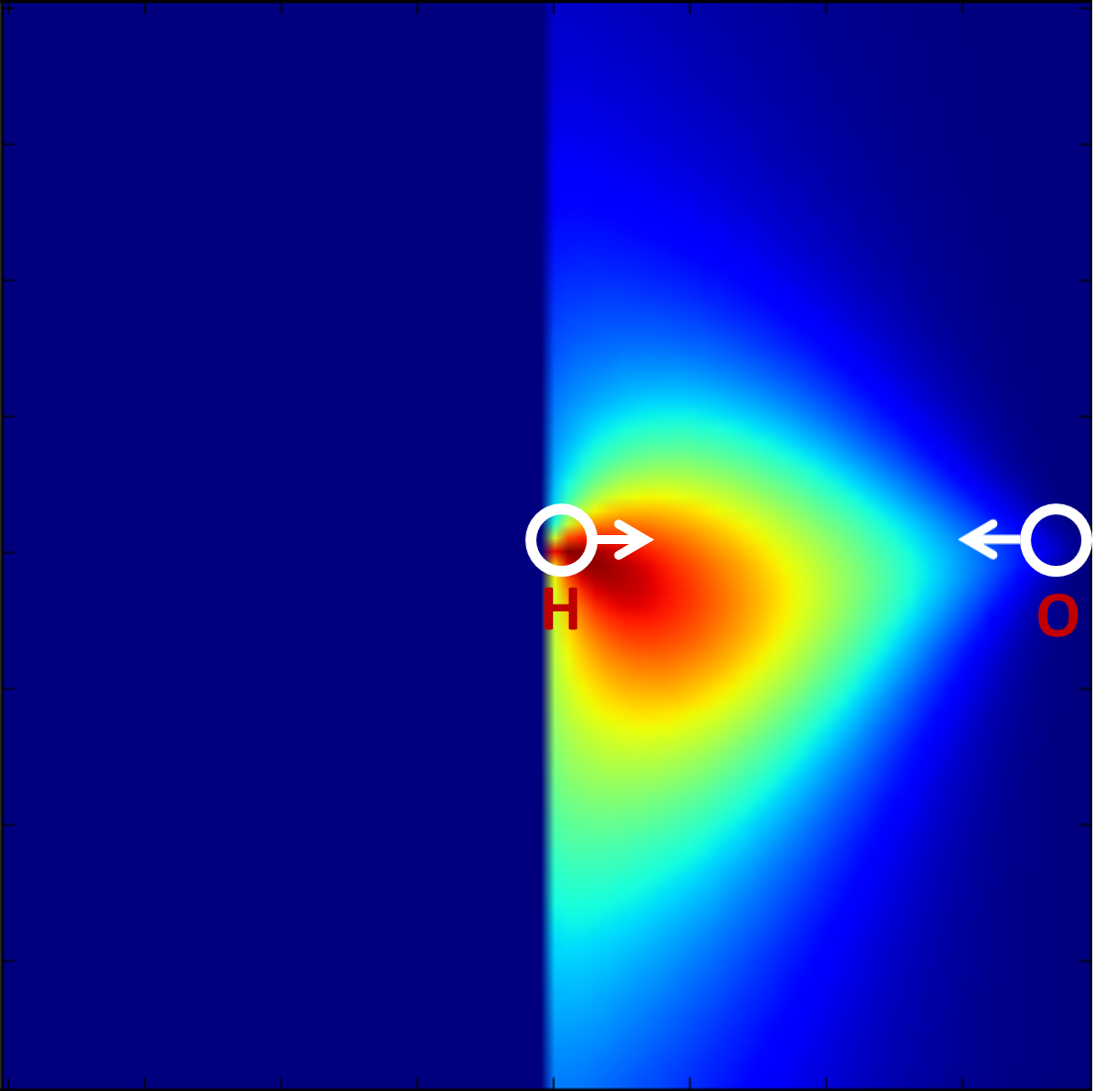
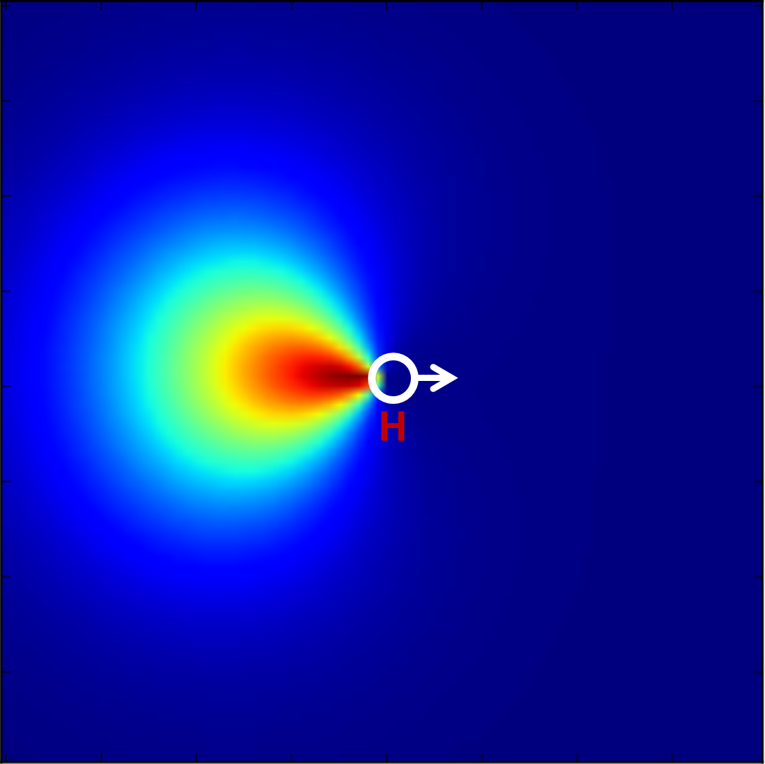
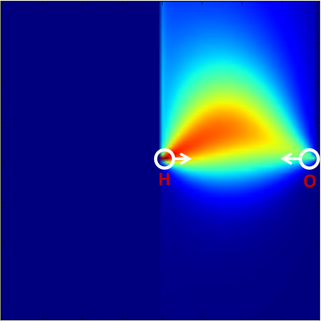
Specifically, we learn the spatial distribution of the human-object interactions. For example, a TV has a watchable affordance and therefore the space between the human and the TV is relevant for the watching activity. Since a watchable label by itself is not informative enough to help in planning we ground it to a spatial distribution. Fig. 6(a) illustrates the learned spatial distribution when the human watches TV. Similarly, a chair is sittable and moveable, but when in use the space behind the chair is critical (because the human sitting on it might move back).

(a) Interacting

(b) Watching

Figure 5: Result of learned edge preference. Distance between human and object is normalized to 1. Human is at 0 and object at 1. For interacting activity, edge preference is symmetric between two humans, but for watching activity humans do not prefer the robot passing very close to them.

(a) Watching

(b) Interacting

(c) Working

Figure 6: An example the learned planning affordance. In the top-view, the human is at the center and facing the object on the right (1m away). Dimension is 2m$\times$2m. (Best viewed in color)

We consider the planning affordance for several activities (e.g., watching, interacting, working, sitting, etc.). For each activity we model a separate cost function $\Psi_{a}$ and evaluate trajectories using Eq. (1). We consider two classes of activities: in the first, the human and object are in close proximity (sitting, working, reaching etc.) and in the second, they are at a distance (walking, watching, interacting etc.). The affordance varies with the distance and angle between the human and the object. We parameterize the cost as follows:

$$\Psi_{a}(t_{i}|E)=\begin{cases}\Psi_{a,ang,h}\;\Psi_{a,ang,o}\;\Psi_{a,\beta}\\ \text{if }a\in\text{activities with human and}\\ \text{\;\;\;\;\;\;\;\;\;\;object at distance.}\\ \\ \Psi_{a,ang,h}\;\Psi_{a,dist,h}\\ \text{if }a\in\text{activities with human and}\\ \text{\;\;\;\;\;\;\;\;\;\;object in close proximity.}\end{cases}$$ (2)

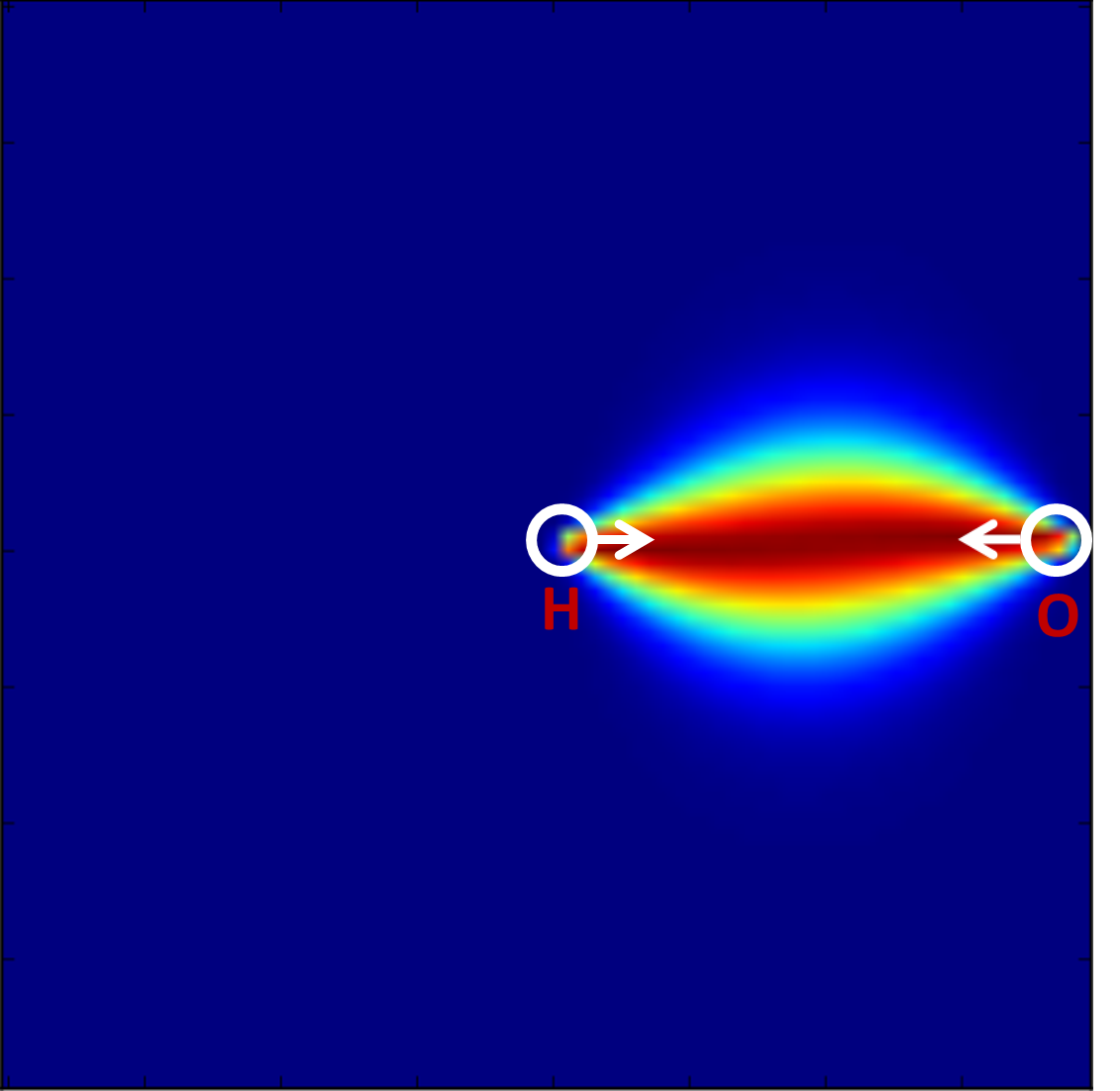
Angular preference $\Psi_{a,ang}(\cdot)$: Certain angular positions w.r.t. the human and the object are more relevant for certain activities. For example, the spatial distribution for the watching activity is spread over a wider angle than the interacting activity (see Fig. 6). We capture the angular distribution of the activity in the space separating the human and the object with two cost functions $\Psi_{a,ang,h}$ and $\Psi_{a,ang,o}$, centered at human and object respectively. For activities with close-proximity between the human and the object we define a single cost centered at human. We parameterize the angular preference cost using the von-Mises distribution as:

$$\Psi_{a,ang,(\cdot)}(\mathbf{x}_{t_{i}};\mu,\kappa)=\frac{1}{2\pi I_{0}(\kappa)}\exp(\kappa\mu^{T}\mathbf{x}_{t_{i}})$$ (3)

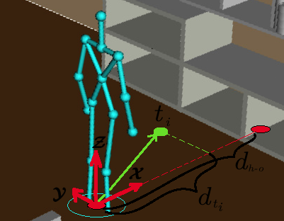
In the above equation, $\mu$ and $\kappa$ are parameters that we will learn from the data, and $\mathbf{x}_{t_{i}}$ is a two-dimensional unit vector. As illustrated in Fig. 7, we obtain $\mathbf{x}_{t_{i}}$ by projecting the waypoint $t_{i}$ onto the co-ordinate frame ($x$ and $y$ axis) defined locally for the human-object activity.

Figure 7: Human side of local co-ordinate system for watching activity. Similar co-ordinates are defined for the object human interacts with. Unit vector $\mathbf{x}_{t_{i}}$ is the projection of waypoint $t_{i}$ on $x$-$y$ axis and normalized it by its length. Distance between human and object is $d_{h-o}$, and $t_{i}$ projected on $x$-axis is of length $d_{t_{i}}$.

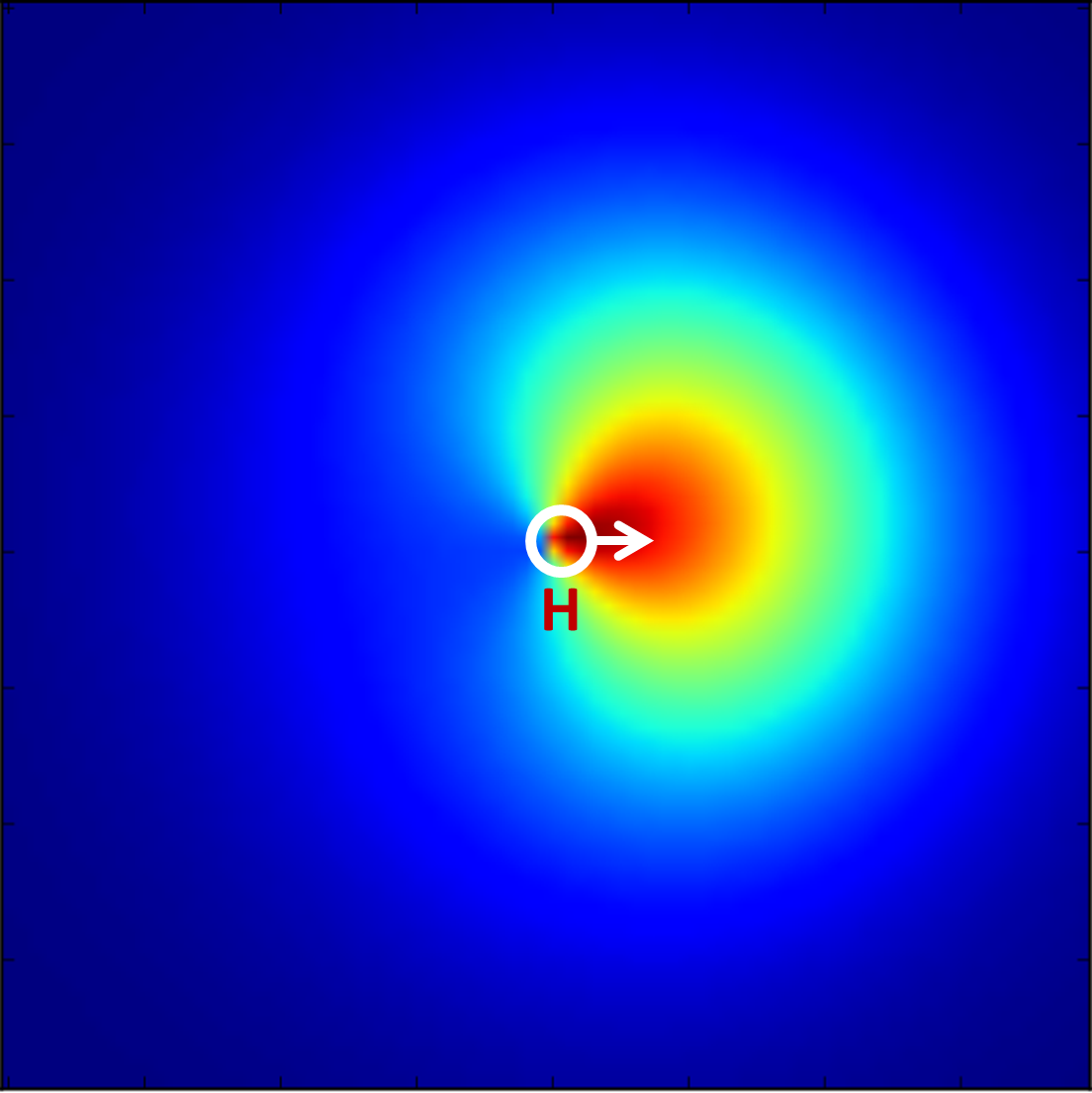
Distance preference $\Psi_{a,dist}$: The preferences vary with the robot distance from the human and the object. Humans do not prefer robots very close to them, especially when the robot is right-in-front or passes from behind [4]. Fig. 6c shows the cost function learned by PlanIt. It illustrates that working humans do not prefer robots passing them from behind. We capture this by adding a 1D-Gaussian parameterized by a mean and variance, and centered at human.
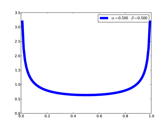
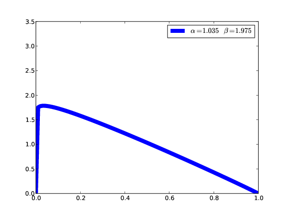
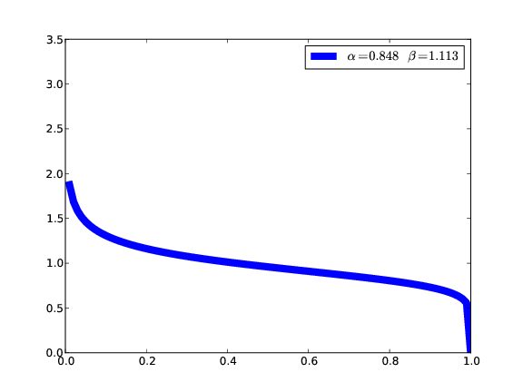
  Edge preference $\Psi_{a,\beta}$: For activities where the human and the object are separated by a distance, the preferences vary along the line connecting human and object. We parameterize this cost using a beta distribution which captures the relevance of the activity along the human-object edge. Fig. 5 illustrates that in the watching activity users prefer robots to cross farther away from them, whereas for the interacting activity the preference is symmetric w.r.t. the humans. To calculate this cost for the waypoint $t_{i}$, we first take its distance from the human and project it along the line joining the human and the object $d_{t_{i}}$, and then normalize it by the distance $d_{h-o}$ between the human and the object. The normalized distance is $\bar{d}_{t_{i}}=d_{t_{i}}/d_{h-o}$. In the equation below, we learn the parameters $\alpha$ and $\beta$.

$$\Psi_{a,\beta}(\bar{d}_{t_{i}};\alpha,\beta)=\frac{\bar{d}_{t_{i}}^{\alpha-1}(1-\bar{d}_{t_{i}})^{\beta-1}}{\text{B}(\alpha,\beta)};\;\;\bar{d}_{t_{i}}\in[0,1]$$ (4)

The functions used in Eq. (1) thus define our cost function. This, however, has many parameters (30) that need to be learned from data.

V-B Generative Model: Learning the Parameters

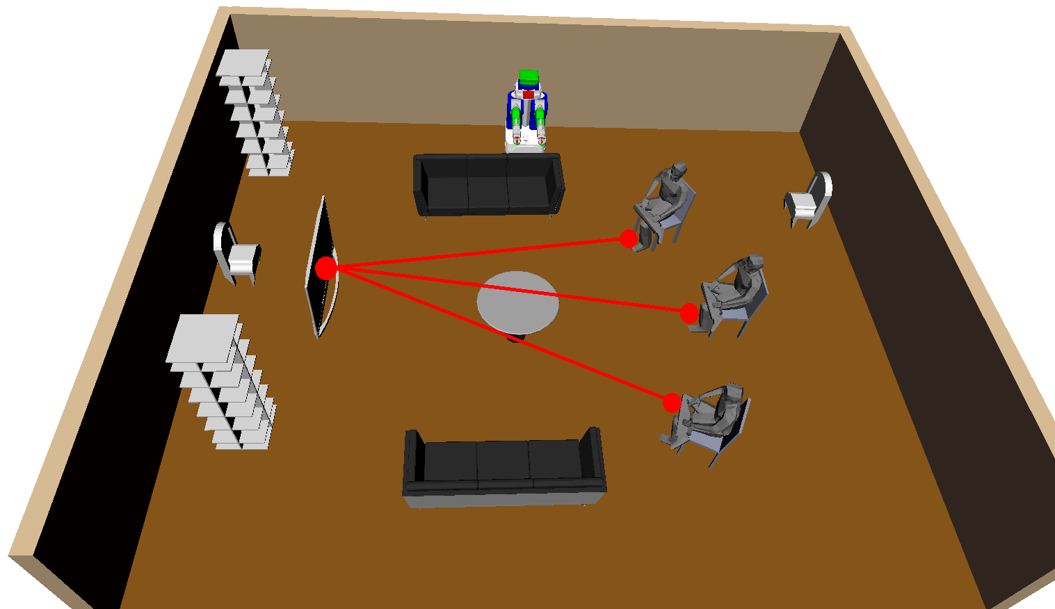
Given the user preference data from PlanIt we learn the parameters of Eq. (1). In order to keep the data collection easy we only elicit labels (bad, neutral or good) on the segments of the videos. The users do not reveal the human activity they think is being affected by the trajectory waypoint they labeled. In fact a waypoint can influence multiple activities. As illustrated in Fig. 8 a waypoint between the humans and the TV can affect multiple watching activities.

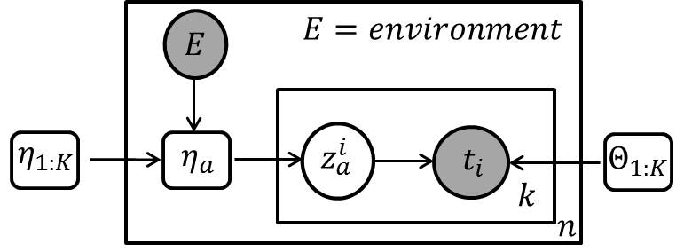
We define a latent random variable $z_{a}^{i}\in\{0,1\}$ for the waypoint $t_{i}$; which is $1$ when the waypoint $t_{i}$ affects the activity $a$ and $0$ otherwise. From the user preference data we learn the following cost function:

$$\mathbf{\Psi}(\{t_{1},..,t_{k}\}|E)=\prod_{i=1}^{k}\underbrace{\sum_{a\in\mathcal{A}_{E}}p(z_{a}^{i}|E)\;\Psi_{a}(t_{i}|E)}_{\text{Marginalizing latent variable $z_{a}^{i}$}}$$ (5)

In the above equation, $p(z_{a}^{i}|E)$ (denoted with $\eta_{a}$) is the (prior) probability of user data arising from activity $a$, and $\mathcal{A}_{E}$ is the set of activities in environment $E$. Fig. 9 shows the generative process for preference data.

Figure 8: Watching activity. Three humans watching a TV.

Figure 9: Feedback model. Generative model of the user preference data.

Training data: We obtain users preferences over $n$ environments $E_{1},..,E_{n}$. For each environment $E$ we consider $m$ trajectory segments $\mathcal{T}_{E,1},..,\mathcal{T}_{E,m}$ labeled as bad by users. For each segment $\mathcal{T}$ we sample $k$ waypoints $\{t_{\mathcal{T},1},..,t_{\mathcal{T},k}\}$. We use $\Theta\in\mathbb{R}^{30}$ to denote the model parameters and solve the following maximum likelihood problem:

$$\Theta^{*} =\arg\max_{\Theta}\prod_{i=1}^{n}\prod_{j=1}^{m}\mathbf{\Psi}(\mathcal{T}_{E_{i},j}|E_{i};\Theta)$$

$$=\begin{multlined}\arg\max_{\Theta}\prod_{i=1}^{n}\prod_{j=1}^{m}\prod_{l=1}^{k}\sum_{a\in\mathcal{A}_{E_{i}}}\;p(z_{a}^{l}|E_{i};\Theta)\\ \Psi_{a}(t_{\mathcal{T}_{E_{i},j},l}|E_{i};\Theta)\end{multlined}\arg\max_{\Theta}\prod_{i=1}^{n}\prod_{j=1}^{m}\prod_{l=1}^{k}\sum_{a\in\mathcal{A}_{E_{i}}}\;p(z_{a}^{l}|E_{i};\Theta)\\ \Psi_{a}(t_{\mathcal{T}_{E_{i},j},l}|E_{i};\Theta)$$ (8)

Eq. (8) does not have a closed form solution. We follow the Expectation-Maximization (EM) procedure to learn the model parameters. In the E-step we calculate the posterior activity assignment $p(z_{a}^{l}|t_{\mathcal{T}_{E_{i},j},l},E_{i})$ for all the waypoints, and in the M-step we update the parameters.

E-step: In this step, with fixed model parameters, we calculate the posterior probability of an activity being affected by a waypoint, as follows:

$$p(z_{a}|t,E;\Theta)=\frac{p(z_{a}|E;\Theta)\Psi_{a}(t|E;\Theta)}{\sum_{a\in\mathcal{A}_{E}}p(z_{a}|E;\Theta)\Psi_{a}(t|E;\Theta)}$$ (9)

We calculate the above probability for every activity $a$ and the waypoint $t$ labeled by users in our data set.

M-step: Using the probabilities calculated in the E-step we update the model parameters in the M-step. Our affordance representation consists of three distributions, namely: Gaussian, von-Mises and Beta. We update the parameters of the Gaussian, and the mean ($\mu$) of the von-Mises in closed form. To update the variance ($\kappa$) of the von-Mises we follow the first order approximation proposed by Sra [41]. Finally the parameters of the beta distribution ($\alpha$ and $\beta$) are updated approximately by using the first and the second order moments of the data. As an example below we give the M-step update of the mean $\mu_{a}$ of the von-Mises.

$$\mu_{a}=\frac{\sum_{i=1}^{n}\sum_{j=1}^{m}\sum_{l=1}^{k}p(z_{a}^{l}|\{t_{\mathcal{T}_{E_{i},j},l}\},E_{i})\mathbf{x}_{\{t_{\mathcal{T}_{E_{i},j},l}\}}}{\|\sum_{i=1}^{n}\sum_{j=1}^{m}\sum_{l=1}^{k}p(z_{a}^{l}|\{t_{\mathcal{T}_{E_{i},j},l}\},E_{i})\mathbf{x}_{\{t_{\mathcal{T}_{E_{i},j},l}\}}\|}$$ (10)

We provide the detailed derivation of the E and M-step in the supplementary material.

VI Experiments and Results

Our data set consists of 122 context-rich 3D-environments that resemble real living rooms or bedrooms. We create them by downloading 2D-images of real environments from the Google images and reconstructing their corresponding 3D models using OpenRAVE [13]. We depict human activities by adding to the 3D models different human poses obtained from the Kinect (refer Fig. 3 in [29] for the human poses). In our experiments we consider six activities: walking, watching, interacting, reaching, sitting and working as shown in Fig. 1.

For these environments we generate trajectory videos and add them to the PlanIt database. We crowdsource 2500 trajectory videos through PlanIt and for each trajectory a user labeled segments of it as bad, neutral or good, corresponding to the scores 1, 3 and 5 respectively.

Figure 10: Examples from our dataset: four living room and two bedroom environments. On left is the 2D image we download from Google images. On right are the 3D reconstructed environments in OpenRAVE. All environments are rich in the types and number of objects and often have multiple humans perform different activities. (Best view: Zoom and view in color)

VI-A Baseline algorithms

We consider the following baseline cost functions:

• Chance: Uniformly randomly assigns a cost in interval [0,1] to a trajectory.

• Maximum Clearance Planning (MCP): Inspired by Sisbot et al. [4], this heuristic favors trajectories which stay farther away from objects. The MCP cost of a trajectory is the (negated) root mean square distance from the nearest object across the trajectory waypoints.

• Human Interference Count (HIC): HIC cost of a trajectory is the number of times it interferes with human activities. Interfering rules were hand designed on expert’s opinion.

• Metropolis Criterion Costmap (MCC): Similar to Mainprice et al. [6], a trajectory’s cost exponentially increases with its closeness to surrounding objects. The MCC cost of a trajectory is defined as follows: $c_{t_{i}}=\min_{o\in\mathcal{O}}dist(t_{i},o)$

  $$\Psi_{mc}(t_{i}) =\begin{cases}e^{-c_{t_{i}}}&c_{t_{i}}<1m\\ 0&\text{otherwise}\end{cases}$$

  $$MCC(\mathcal{T}=\{t_{1},..,t_{n}\}) =\frac{\sum_{i=1}^{n}\Psi_{mc}(t_{i})}{n}$$

  $dist(t_{i},o)$ is the euclidean distance between the waypoint $t_{i}$ and the object $o$.

• HIC scaled with MCC: We design this heuristic by combining the HIC and the MCC costs. The HICMCC cost of a trajectory is $HICMCC(\mathcal{T})=MCC(\mathcal{T})*HIC(\mathcal{T})$

• Trajectory Preference Perceptron (TPP): Jain et al. [32] learns a cost function from co-active user feedback in an online setting. We compare against the TPP using trajectory features from [32].

The above described baselines assign cost to trajectories and lower cost is preferred. For quantitative evaluation each trajectory is also assigned a ground truth score based on the user feedback from PlanIt. The ground truth score of a trajectory is the minimum score given by a user. For example if two segments of a trajectory are labeled with scores 3 (neutral) and 5 (good), then the ground truth score is 3. We denote the ground truth score of trajectory $\mathcal{T}$ as $score(\mathcal{T})$.

VI-B Evaluation Metric

Given the ground truth scores we evaluate algorithms based on the following metrics.

• Misclassification rate: For a trajectory $\mathcal{T}_{i}$ we consider the set of trajectories $\mathbf{T}_{i}$ with higher ground truth score: $\mathbf{T}_{i}=\{\mathcal{T}|score(T)>score(\mathcal{T}_{i})\}$. The misclassification rate of an algorithm is the number of trajectories in $\mathbf{T}_{i}$ which it assigns a higher cost than $\mathcal{T}_{i}$. We normalize this count by the number of trajectories in $\mathbf{T}_{i}$ and average it over all the trajectories $\mathcal{T}_{i}$ in the data set. Lower misclassification rate is desirable.

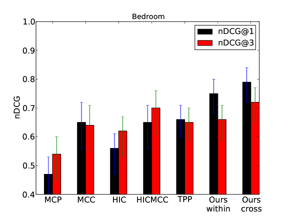
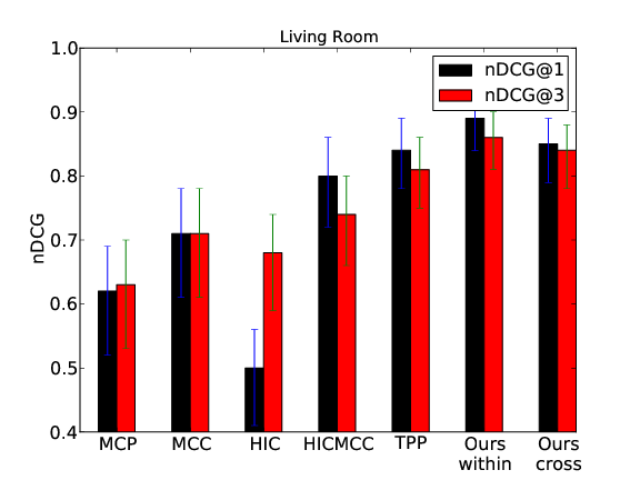
• Normalized discounted cumulative gain (nDCG) [42]: This metric quantifies how well an algorithm rank trajectories. It is a relevant metric because autonomous robots can rank trajectories and execute the top ranked trajectory [43, 32]. Obtaining a rank list simply amounts to sorting the trajectories based on their costs.

VI-C Results

We evaluate the trained model for its:

• Discriminative power: How well can the model distinguish good/bad trajectories?

• Interpretability: How well does the qualitative visualization of the cost function heatmaps match our intuition?

VI-D Discriminative power of learned cost function

Figure 11: Crowdsourcing improves performance: Misclassification rate decreases as more users provide feedback via PlanIt.

A model trained on users preferences should reliably distinguish good from bad trajectories i.e. if we evaluate two trajectories under the learned model then it should assign a lower cost to the better trajectory. We compare algorithms under two training settings: (i) within-env: we test and train on the same category of environment using 5-fold cross validation, e.g. training on bedrooms and testing on new bedrooms; and (ii) cross-env: we train on bedrooms and test on living rooms, and vice-versa. In both settings the algorithms were tested on environments not seen before.

Table I: Misclassification rate: chances that an algorithm presented with two trajectories (one good and other bad) orders them incorrectly. Lower rate is better. The number inside bracket is standard error.

Algorithms	Bedroom	Living room
Chance	.52 (-)	.48 (-)
MCP based on Sisbot et al. [4]	.46 (.04)	.42 (.06)
MCC based on Mainprice et al. [6]	.44 (.03)	.42 (.06)
HIC	.30 (.04)	.23 (.06)
HICMCC	.32 (.04)	.29 (.05)
TPP based on Jain et al. [32]	.33 (.03)	.34 (.05)
Ours within scenario evaluation	.32 (.05)	.19 (.03)
Ours cross scenario evaluation	.27 (.04)	.17 (.05)

Figure 12: nDCG plots comparing algorithms on bedroom (left) and living room (right) environments. Error bar indicates standard error.

How well algorithms discriminate between trajectories? We compare algorithms on the evaluation metrics described above. As shown in Table I our algorithm gives the lowest misclassification rate in comparison to the baseline algorithms. We also observe that the misclassification rate on bedrooms is lower with cross-env training than within-env. We conjecture this is because of a harder learning problem (on average) when training on bedrooms than living rooms. In our data set, on average a bedroom have 3 human activities while a living room have 2.06. Therefore the model parameters converge to better optima when trained on living rooms. As illustrated in Fig. 12, our algorithm also ranks trajectories better than other baseline algorithms.
 
  Crowdsourcing helps and so does learning preferences! We compare our approach to TPP learning algorithm by Jain et al. [32]. TPP learns with co-active feedback which requires the user to iteratively improve the trajectory proposed by the system. This feedback is time consuming to elicit and therefore difficult to scale to many environments. On both evaluation metrics our crowdsourcing approach outperforms TPP, which is trained on fewer environments. 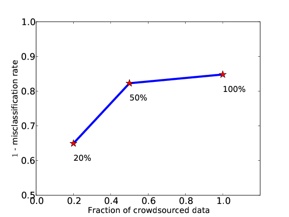Fig. 11 shows our model improves as users provide more feedback through PlanIt. Our data-driven approach is also a better alternative to hand-designed cost functions.

Figure 13: Robotic experiment: A screen-shot of our algorithm running on PR2. Without learning robot blocks view of human watching football. http://planit.cs.cornell.edu/video

(a) Edge preference for walking

(b) Walking

(c) Sitting

Figure 14: Learned affordance heatmaps. (a) Edge preference for walking activity. Human is at 0 and object at 1. (b,c) Top view of heatmaps. Human is at the center and facing right.

(a) Bedroom

(b) Planning affordance

Figure 15: Planning affordance map for an environment. Bedroom with sitting, reaching and watching activities. A robot uses the affordance map as a cost for planning good trajectories.

VI-E Interpretability: Qualitative visualization of learned cost

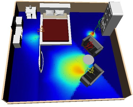
Visualizing the learned heatmaps is useful for understanding the spatial distribution of human-object activities. We discussed the learned heatmaps for watching, interacting and working activities in Section V-A (see Fig. 6). Fig. 14 illustrates the heatmap for the walking, and sitting activities.
 
  How does crowd preferences change with the nature of activity? For the same distance between the human and the object, the spatial preference learned from the crowd is less-spread for interacting activity than watching and walking activities, as shown in Fig. 6. This empirical evidence implies that while interacting humans do not mind the robot in vicinity unless it blocks their eye contact.

The preferences also vary along the line joining the human and object. As shown in Fig. 5, while watching TV the space right in front of the human is critical, and the edge-preference rapidly decays as we move towards the TV. On the other hand, when human is walking towards an object the decay in edge-preference is slower, Fig. 14(a).
 
  Using the PlanIt system and the cost map of individual activities, a.k.a. affordance library, we generate the planning map of environments with multiple activities. Some examples of the planning map are shown in Fig. 15.

VI-F Robotic Experiment: Planning via PlanIt

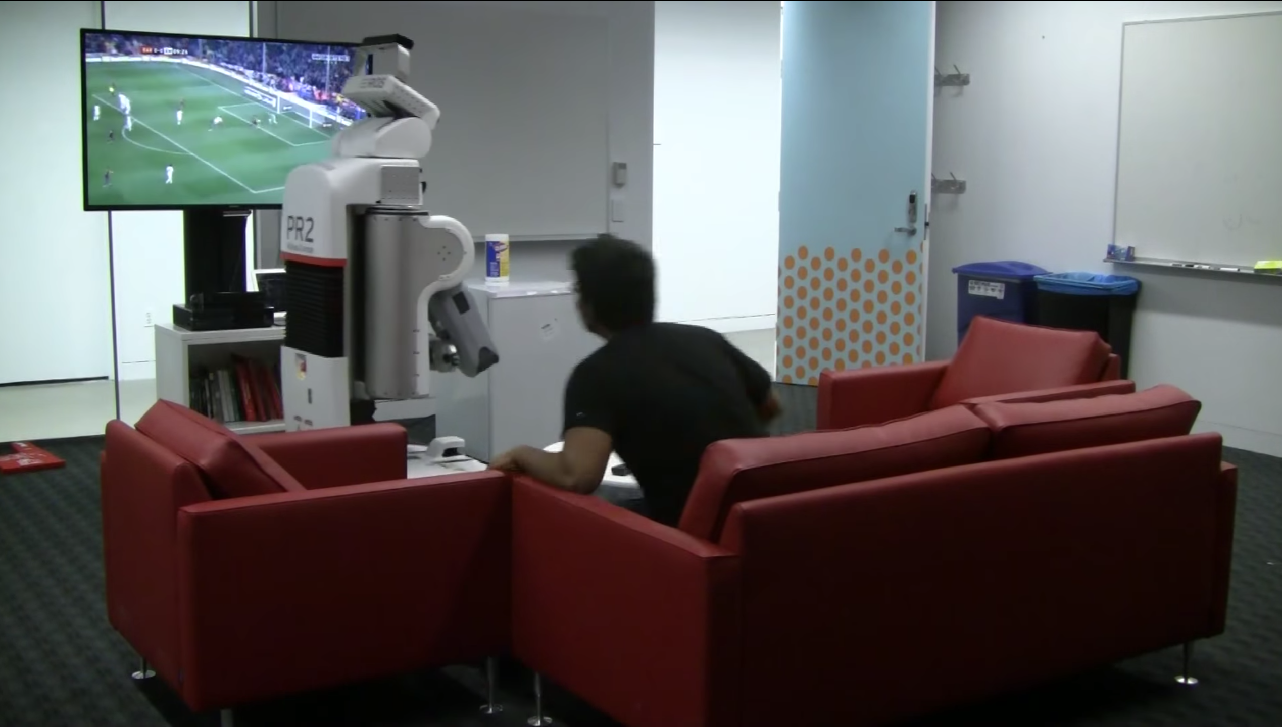
In order to plan trajectories in an unseen environment we generate its planning map and use it as an input cost to the RRT [17] planner. Given the cost function, RRT plans trajectories with low cost. We implement our learned model on PR2 robot for the purpose of navigation when the human is watching a football match on the TV (Fig. 13). Without learning the preferences, the robot plans the shortest path to the goal and obstructs the human’s view of TV. Demonstration: http://planit.cs.cornell.edu/video

VI-G Application to manipulation tasks

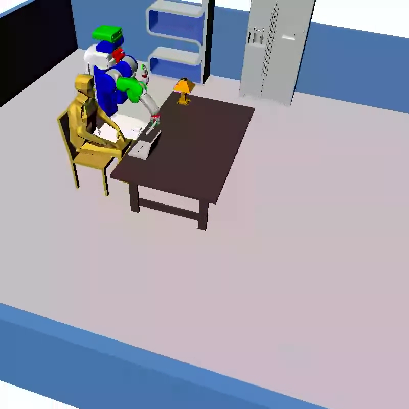
We also apply our model to manipulation tasks which requires modeling higher dimensional state space involving object and robot-arm configurations. We consider tasks involving object-object interactions such as, manipulating sharp objects in human vicinity or moving a glass of water near electronic devices. For such tasks one has to model both the object’s distance from its surrounding and its orientation.

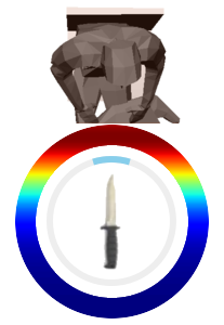
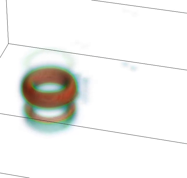
Similar to navigation, we show videos on PlanIt of robot manipulating objects such as a knife in the vicinity of humans and other objects. As feedback users label segments of videos as good/bad/neutral, we model the feedback as a generative process shown in Fig. 9. We parametrize the cost function using Gaussian, von-Mises and Beta distributions. More details on parameterization and EM updates are in the supplementary material. Fig. 16 shows learned preference for manipulating a knife in human vicinity. We learn that humans prefer the knife pointing away from them. The learned heatmap is dense near the face implying humans strongly prefer the knife far away from their face.

Figure 16: Learned heatmap for manipulation. (Left) Robot manipulating knife in presence of human and laptop. (Middle) Learned heatmap showing preferred orientation of knife w.r.t. human – red being the most unpreferred orientation. (Right) 3D heat cloud of the same room showing undesirable positions of knife when its orientation is fixed to always point at the human. Heatmap has higher density near the face. (Best viewed in color. See interactive version at the PlanIt website.)

VI-H Sharing the learned concepts

In order to make the knowledge from PlanIt useful to robots, we have partnered with RoboBrain [44] – an ongoing open-source research effort. The RoboBrain represents the information relevant for robots in form of a knowledge graph. The concepts learned by PlanIt are connected to its knowledge graph. The planning affordances learned by PlanIt are represented as nodes in the graph and they are connected (with edges) to their associated human activity node. This way PlanIt enables RoboBrain to connect different types of affordances associated with an activity. For example, the planning affordance when moving a knife and its grasping affordance [24] are related through cutting activity.

VII Conclusion

In this paper we proposed a crowdsourcing approach for learning user preferences over trajectories. Our PlanIt system is user-friendly and easy-to-use for eliciting large scale preference data from non-expert users. The simplicity of PlanIt comes at the expense of weak and noisy labels with latent annotator intentions. We presented a generative approach with latent nodes to model the preference data. Through PlanIt we learn spatial distribution of activities involving humans and objects. We experimented on many context-rich living and bedroom environments. Our results validate the advantages of crowdsourcing and learning the cost over hand encoded heuristics. We also implemented our learned model on the PR2 robot. PlanIt is publicly available for visualizing learned cost function heatmaps, viewing robotic demonstration, and providing preference feedback http://planit.cs.cornell.edu.
 
  Acknowledgement This work was supported in part by ARO and by NSF Career Award to Saxena.

References

- [1] S. Karaman and E. Frazzoli, “Incremental sampling-based algorithms for optimal motion planning,” in RSS, 2010.
- [2] N. Ratliff, M. Zucker, J. A. Bagnell, and S. Srinivasa, “Chomp: Gradient optimization techniques for efficient motion planning,” in ICRA, 2009.
- [3] J. Schulman, J. Ho, A. Lee, I. Awwal, H. Bradlow, and P. Abbeel, “Finding locally optimal, collision-free trajectories with sequential convex optimization,” in RSS, 2013.
- [4] E. A. Sisbot, L. F. Marin-Urias, R. Alami, and T. Simeon, “A human aware mobile robot motion planner,” IEEE Transactions on Robotics, 2007.
- [5] E. A. Sisbot and R. Alami, “A human-aware manipulation planner,” Robotics, IEEE Transactions on, vol. 28, 2012.
- [6] J. Mainprice, E. A. Sisbot, L. Jaillet, J. Cortés, R. Alami, and T. Siméon, “Planning human-aware motions using a sampling-based costmap planner,” in ICRA, 2011.
- [7] A. Jain, S. Sharma, and A. Saxena, “Beyond geometric path planning: Learning context-driven user preferences via sub-optimal feedback,” in ISRR, 2013.
- [8] J. J. Gibson, The ecological approach to visual perception. Routledge, 1986.
- [9] E. Şahin, M. Çakmak, M. R. Doğar, E. Uğur, and G. Üçoluk, “To afford or not to afford: A new formalization of affordances toward affordance-based robot control,” Adaptive Behavior, vol. 15, no. 4, pp. 447–472, 2007.
- [10] L. Montesano, M. Lopes, A. Bernardino, and J. S.-Victor, “Learning object affordances: from sensory–motor coordination to imitation,” IEEE Transactions on Robotics, 2008.
- [11] H. Koppula, R. Gupta, and A. Saxena, “Learning human activities and object affordances from rgb-d videos,” IJRR, vol. 32, no. 8, 2013.
- [12] D. Katz, A. Venkatraman, M. Kazemi, J. A. Bagnell, and A. Stentz, “Perceiving, learning, and exploiting object affordances for autonomous pile manipulation,” in RSS, 2013.
- [13] R. Diankov, “Automated construction of robotic manipulation programs,” Ph.D. dissertation, CMU, RI, August 2010.
- [14] P. Abbeel, A. Coates, and A. Y. Ng, “Autonomous helicopter aerobatics through apprenticeship learning,” IJRR, vol. 29, no. 13, 2010.
- [15] J. Kober and J. Peters, “Policy search for motor primitives in robotics,” ML, vol. 84, no. 1, 2011.
- [16] N. Ratliff, J. A. Bagnell, and M. Zinkevich, “Maximum margin planning,” in ICML, 2006.
- [17] S. M. LaValle and J. J. Kuffner, “Randomized kinodynamic planning,” IJRR, vol. 20, no. 5, 2001.
- [18] D. D. Ferguson and A. Stentz, “Anytime rrts,” in IROS, 2006.
- [19] L. Jaillet, J. Cortés, and T. Siméon, “Sampling-based path planning on configuration-space costmaps,” IEEE TRO, vol. 26, no. 4, 2010.
- [20] P. Leven and S. Hutchinson, “Using manipulability to bias sampling during the construction of probabilistic roadmaps,” IEEE Trans. on Robotics and Automation, vol. 19, no. 6, 2003.
- [21] M. Bennewitz, W. Burgard, G. Cielniak, and S. Thrun, “Learning motion patterns of people for compliant robot motion,” IJRR, 2005.
- [22] M. Kuderer, H. Kretzschmar, C. Sprunk, and W. Burgard, “Feature-based prediction of trajectories for socially compliant navigation,” in RSS, 2012.
- [23] B. D. Ziebart, N. Ratliff, G. Gallagher, C. Mertz, K. Peterson, J. A. Bagnell, M. Hebert, A. K. Dey, and S. Srinivasa, “Planning-based prediction for pedestrians,” in IROS, 2009.
- [24] H. Koppula and A. Saxena, “Anticipating human activities using object affordances for reactive robotic response,” in RSS, 2013.
- [25] J. Mainprice and D. Berenson, “Human-robot collaborative manipulation planning using early prediction of human motion,” in IROS, 2013.
- [26] Z. Wang, K. Mülling, M. Deisenroth, H. Amor, D. Vogt, B. Schölkopf, and J. Peters, “Probabilistic movement modeling for intention inference in human-robot interaction,” IJRR, 2013.
- [27] E. Ugur, E. Oztop, and E. Sahin, “Goal emulation and planning in perceptual space using learned affordances,” Robotics and Autonomous Systems, 2011.
- [28] K. F. Uyanik, Y. Caliskan, A. K. Bozcuoglu, S. K. O. Yuruten, and E. Sahin, “Learning social affordances and using them for planning,” in CogSys, 2013.
- [29] Y. Jiang, M. Lim, and A. Saxena, “Learning object arrangements in 3d scenes using human context,” in ICML, 2012.
- [30] E. A. Sisbot, L. F. Marin, and R. Alami, “Spatial reasoning for human robot interaction,” in IROS, 2007.
- [31] A. Dragan, K. Lee, and S. Srinivasa, “Legibility and predictability of robot motion,” in HRI, 2013.
- [32] A. Jain, B. Wojcik, T. Joachims, and A. Saxena, “Learning trajectory preferences for manipulators via iterative improvement,” in NIPS, 2013.
- [33] M. J. Y. Chung, M. Forbes, M. Cakmak and R. P. Rao, “Accelerating imitation learning through crowdsourcing,” in ICRA, 2014.
- [34] N. Curtis and J. Xiao, “Efficient and effective grasping of novel objects through learning and adapting a knowledge base,” in IROS, 2008.
- [35] A. T. Miller and P. K. Allen, “Graspit! a versatile simulator for robotic grasping,” Robotics & Automation Magazine, IEEE, vol. 11, no. 4, 2004.
- [36] R. Paolini, A. Rodriguez, S. S. Srinivasa, and M. T. Mason, “A data-driven statistical framework for post-grasp manipulation,” in ISER, 2013.
- [37] D. Katz, Y. Pyuro, and O. Brock, “Learning to manipulate articulated objects in unstructured environments using a grounded relational representation,” in RSS, 2008.
- [38] P. Vernaza and J. A. Bagnell, “Efficient high dimensional maximum entropy modeling via symmetric partition functions,” in NIPS, 2012.
- [39] B. Akgun, M. Cakmak, K. Jiang, and A. L. Thomaz, “Keyframe-based learning from demonstration,” IJSR, vol. 4, no. 4, pp. 343–355, 2012.
- [40] J. V. D. Berg, P. Abbeel, and K. Goldberg, “Lqg-mp: Optimized path planning for robots with motion uncertainty and imperfect state information,” in RSS, 2010.
- [41] S. Sra, “A short note on parameter approximation for von mises-fisher distributions: and a fast implementation of i s (x),” Computational Statistics, vol. 27, no. 1, 2012.
- [42] C. D. Manning, P. Raghavan, and H. Schütze, Introduction to information retrieval. Cambridge University Press Cambridge, 2008, vol. 1.
- [43] D. Dey, T. Y. Liu, M. Hebert, and J. A. Bagnell, “Contextual sequence prediction with application to control library optimization,” in RSS, 2012.
- [44] A. Saxena, A. Jain, O. Sener, A. Jami, D. K. Misra, H. S. Koppula, “RoboBrain: Large-Scale Knowledge Engine for Robots,” arXiv preprint arXiv:1412.0691, 2014