Multilevel path simulation for weak approximation schemes

Denis Belomestny111This research was partially supported by the Deutsche Forschungsgemeinschaft through the SPP 1324 “Mathematical methods for extracting quantifiable information from complex systems” and by Laboratory for Structural Methods of Data Analysis in Predictive Modeling, MIPT, RF government grant, ag. 11.G34.31.0073. and Tigran Nagapetyan
Duisburg-Essen University, National Research University Higher School of Economics, Weierstrass Institute for Applied Analysis and Stochastics

In this paper we discuss the possibility of using multilevel Monte Carlo (MLMC) methods for weak approximation schemes. It turns out that by means of a simple coupling between consecutive time discretisation levels, one can achieve the same complexity gain as under the presence of a strong convergence. We exemplify this general idea in the case of weak Euler scheme for Lévy driven stochastic differential equations, and show that, given a weak convergence of order α1/2,𝛼12\alpha\geq 1/2, the complexity of the corresponding “weak” MLMC estimate is of order ε2log2(ε).superscript𝜀2superscript2𝜀\varepsilon^{-2}\log^{2}(\varepsilon). The numerical performance of the new “weak” MLMC method is illustrated by several numerical examples.

\abslabeldelim

Multilevel path simulation for weak approximation schemes

Denis Belomestny222This research was partially supported by the Deutsche Forschungsgemeinschaft through the SPP 1324 “Mathematical methods for extracting quantifiable information from complex systems” and by Laboratory for Structural Methods of Data Analysis in Predictive Modeling, MIPT, RF government grant, ag. 11.G34.31.0073. and Tigran Nagapetyan
Duisburg-Essen University, National Research University Higher School of Economics, Weierstrass Institute for Applied Analysis and Stochastics

1 Introduction

The multilevel path simulation method introduced in Giles [7] has gained huge popularity as a complexity reduction tool in recent times. The main advantage of the MLMC methodology is that it can be simply applied to various situations and requires almost no prior knowledge on the path generating process. Any multilevel Monte Carlo (MLMC) algorithm uses a number of levels of resolution, l=0,1,,L,𝑙01𝐿l=0,1,\ldots,L, with l=0𝑙0l=0 being the coarsest, and l=L𝑙𝐿l=L being the finest. In the context of a SDE simulation on the interval [0,T]0𝑇[0,T], level 00 corresponds to one timestep Δ0=T,subscriptΔ0𝑇\Delta_{0}=T, whereas the level L𝐿L has 2Lsuperscript2𝐿2^{L} uniform timesteps ΔL=2LT.subscriptΔ𝐿superscript2𝐿𝑇\Delta_{L}=2^{-L}T.

Assume that a filtered probability space (Ω,,P,(t))ΩPsubscript𝑡(\Omega,\mathcal{F},\operatorname{P},(\mathcal{F}_{t})) is given. Consider now a d𝑑d-dimensional process (Xt)subscript𝑋𝑡(X_{t}) solving the following Lévy driven SDE

Xt=X0+0ta(Xs)𝑑Ls,subscript𝑋𝑡subscript𝑋0superscriptsubscript0𝑡𝑎subscript𝑋limit-from𝑠differential-dsubscript𝐿𝑠\displaystyle X_{t}=X_{0}+\int_{0}^{t}a(X_{s-})\,dL_{s}, (1.1)

where X0subscript𝑋0X_{0} is a \mathbbRd\mathbbsuperscript𝑅𝑑\mathbb{R}^{d}-valued random variable, Lt=(Lt1,,Ltm),subscript𝐿𝑡subscriptsuperscript𝐿1𝑡subscriptsuperscript𝐿𝑚𝑡L_{t}=(L^{1}_{t},\ldots,L^{m}_{t}), t0𝑡0t\geq 0 is a m𝑚m-dimensional Lévy process and the mapping a::𝑎absenta: \mathbbRd×\mathbbRm\mathbbRdmaps-to\mathbbsuperscript𝑅𝑑\mathbbsuperscript𝑅𝑚\mathbbsuperscript𝑅𝑑\mathbb{R}^{d}\times\mathbb{R}^{m}\mapsto\mathbb{R}^{d} is Lipschitz continuous and has at most linear growth on [0,T]0𝑇[0,T] so that the solution of (1.1) is well defined. Our aim is to estimate the expectation E[f(XT)],Edelimited-[]𝑓subscript𝑋𝑇\mathrm{E}[f(X_{T})], where f𝑓f is a Lipschitz continuous function from \mathbbRd\mathbbsuperscript𝑅𝑑\mathbb{R}^{d} to \mathbbR.\mathbb𝑅\mathbb{R}. Let XTlsubscriptsuperscript𝑋𝑙𝑇X^{l}_{T} be an approximation for XTsubscript𝑋𝑇X_{T} by means of a numerical discretisation with time step ΔlsubscriptΔ𝑙\Delta_{l} (for various discretisation methods for (1.1) see, e. g. Platen and Bruti-Liberati [16] or the recent review of Jourdain and Kohatsu-Higa [11]). The main idea of the multilevel approach pioneered in Giles [7] consists in writing the expectation of the finest approximation E[f(XTL)]Edelimited-[]𝑓subscriptsuperscript𝑋𝐿𝑇\mathrm{E}[f(X^{L}_{T})] as a telescopic sum

E[f(XTL)]=E[f(XT0)]+l=1LE[f(XTl)f(XTl1)]Edelimited-[]𝑓subscriptsuperscript𝑋𝐿𝑇Edelimited-[]𝑓subscriptsuperscript𝑋0𝑇superscriptsubscript𝑙1𝐿Edelimited-[]𝑓subscriptsuperscript𝑋𝑙𝑇𝑓subscriptsuperscript𝑋𝑙1𝑇\displaystyle\mathrm{E}[f(X^{L}_{T})]=\mathrm{E}[f(X^{0}_{T})]+\sum_{l=1}^{L}\mathrm{E}[f(X^{l}_{T})-f(X^{l-1}_{T})]

and then applying Monte Carlo to estimate each expectation in the above telescopic sum. One important prerequisite for MLMC to work is that XTlsubscriptsuperscript𝑋𝑙𝑇X^{l}_{T} and XTl1subscriptsuperscript𝑋𝑙1𝑇X^{l-1}_{T} are coupled in some way and this can be achieved by using the same discretised trajectories of the underlying Lévy processes to construct the consecutive approximations XTlsubscriptsuperscript𝑋𝑙𝑇X^{l}_{T} and XTl1.subscriptsuperscript𝑋𝑙1𝑇X^{l-1}_{T}. The degree of coupling is usually measured in terms of the variance Var[f(XTl)f(XTl1)]Var𝑓subscriptsuperscript𝑋𝑙𝑇𝑓subscriptsuperscript𝑋𝑙1𝑇\operatorname{Var}[f(X^{l}_{T})-f(X^{l-1}_{T})]. It is shown in Giles [7] (see also Giles and Xia [8]), that under the assumptions

|E[f(XTL)]E[f(XT)]|c1ΔLα,Var[f(XTl)f(XTl1)]c2Δlβ,formulae-sequenceEdelimited-[]𝑓subscriptsuperscript𝑋𝐿𝑇Edelimited-[]𝑓subscript𝑋𝑇subscript𝑐1superscriptsubscriptΔ𝐿𝛼Var𝑓subscriptsuperscript𝑋𝑙𝑇𝑓subscriptsuperscript𝑋𝑙1𝑇subscript𝑐2superscriptsubscriptΔ𝑙𝛽\displaystyle\bigl{|}\mathrm{E}[f(X^{L}_{T})]-\mathrm{E}[f(X_{T})]\bigr{|}\leq c_{1}\Delta_{L}^{\alpha},\quad\operatorname{Var}\left[f(X^{l}_{T})-f(X^{l-1}_{T})\right]\leq c_{2}\Delta_{l}^{\beta}, (1.2)

with some α1/2,𝛼12\alpha\geq 1/2, β>0,𝛽0\beta>0, c1>0subscript𝑐10c_{1}>0 and c2>0,subscript𝑐20c_{2}>0, the computational complexity of the resulting multilevel estimate needed to achieve the accuracy ε𝜀\varepsilon (in terms of RMSE) is proportional to

𝒞={ε2,β>1,ε2log2(ε),β=1,ε2(1β)/α,0<β<1.𝒞casessuperscript𝜀2𝛽1superscript𝜀2superscript2𝜀𝛽1superscript𝜀21𝛽𝛼0𝛽1\displaystyle\mathcal{C}=\begin{cases}\varepsilon^{-2},&\beta>1,\\ \varepsilon^{-2}\log^{2}(\varepsilon),&\beta=1,\\ \varepsilon^{-2-(1-\beta)/\alpha},&0<\beta<1.\end{cases}

The standard way of checking the assumptions (1.2) is to prove that the underlying approximation scheme has weak convergence of order α𝛼\alpha and strong convergence of order β/2.𝛽2\beta/2. Indeed, in the latter case we have for any Lipschitz continuous function f,𝑓f,

Var[f(XTl)f(XTl1)]Var𝑓subscriptsuperscript𝑋𝑙𝑇𝑓subscriptsuperscript𝑋𝑙1𝑇\displaystyle\operatorname{Var}\left[f(X^{l}_{T})-f(X^{l-1}_{T})\right] cfE[|XTlXT|2]+cfE[|XTl1XT|2]absentsubscript𝑐𝑓Edelimited-[]superscriptsubscriptsuperscript𝑋𝑙𝑇subscript𝑋𝑇2subscript𝑐𝑓Edelimited-[]superscriptsubscriptsuperscript𝑋𝑙1𝑇subscript𝑋𝑇2\displaystyle\leq c_{f}\mathrm{E}\left[\bigl{|}X^{l}_{T}-X_{T}\bigr{|}^{2}\right]+c_{f}\mathrm{E}\left[\bigl{|}X^{l-1}_{T}-X_{T}\bigr{|}^{2}\right]
2cfΔlβabsent2subscript𝑐𝑓superscriptsubscriptΔ𝑙𝛽\displaystyle\leq 2c_{f}\Delta_{l}^{\beta}

with some constant cf>0subscript𝑐𝑓0c_{f}>0 depending on f.𝑓f. However, in recent years the so-called weak approximation schemes, i.e., schemes that, in general, fulfil only the first assumption in (1.2) became quite popular. The weak Euler scheme is a first-order scheme with α=1𝛼1\alpha=1, and has been studied by many researchers. Talay and Tubaro [19] show the first-order convergence of the weak Euler scheme. The fact that the convergence rate of the Euler scheme also holds for certain irregular functions under a Hörmander type condition has been proved by Bally and Talay [2] using Malliavin calculus. The Itô-Taylor (weak-Taylor) high-order scheme is a natural extension of the weak Euler scheme. In the continuous diffusion case, some new discretization schemes (also called Kusuoka type schemes) which are of order α2𝛼2\alpha\geq 2 without the Romberg extrapolation have been introduced by Kusuoka [12], Lyons and Victoir [13], Ninomiya and Victoir [15], and Ninomiya and Ninomiya [14]. A general class of weak approximation methods, comprising many well known discretisation schemes, was constructed in Kohatsu-Higa and Tanaka [20]. The main advantage of the weak approximation schemes is that simple discrete random variables can be used instead of the Lévy increments. Unfortunately, due to the absence of the strong convergence, the MLMC methodology can not be directly used with the weak approximation schemes. In this paper we make an attempt to overcome this difficulty and develop a kind of “weak” MLMC approach which can be applied to various weak approximation schemes.

The plan of the paper is as follows. First, we recall the Euler scheme for (1.1) and discuss its convergence properties. Next we show how to construct the corresponding MLMC algorithm, which is able to reduce the complexity of the standard MC to order ε2log2(ε)superscript𝜀2superscript2𝜀\varepsilon^{-2}\log^{2}(\varepsilon) under only requirement that the Euler scheme converges weakly. Finally, we analyse the numerical performance of the presented weak MLMC algorithms.

2 Euler scheme for Lévy driven SDE

Fix some n\mathbbN𝑛\mathbb𝑁n\in\mathbb{N} and set Δ=T/n.Δ𝑇𝑛\Delta=T/n. Denote ΔLj=LjΔL(j1)Δ,Δsubscript𝐿𝑗subscript𝐿𝑗Δsubscript𝐿𝑗1Δ\Delta L_{j}=L_{j\Delta}-L_{(j-1)\Delta}, j=1,,n.𝑗1𝑛j=1,\ldots,n. For a fixed random vector X0,subscript𝑋0X_{0}, the Euler scheme for (1.1) reads as follows

X0Δsubscriptsuperscript𝑋Δ0\displaystyle X^{\Delta}_{0} =\displaystyle= X0,subscript𝑋0\displaystyle X_{0}, (2.1)
XjΔΔsubscriptsuperscript𝑋Δ𝑗Δ\displaystyle X^{\Delta}_{j\Delta} =\displaystyle= X(j1)ΔΔ+a(X(j1)ΔΔ)ΔLj,j=1,,n.formulae-sequencesubscriptsuperscript𝑋Δ𝑗1Δ𝑎subscriptsuperscript𝑋Δ𝑗1ΔΔsubscript𝐿𝑗𝑗1𝑛\displaystyle X^{\Delta}_{(j-1)\Delta}+a\bigl{(}X^{\Delta}_{(j-1)\Delta}\bigr{)}\,\Delta L_{j},\quad j=1,\ldots,n.

The convergence of the scheme (2.1) was extensively studied in the literature. The first convergence result is due to Talay and Tubaro [19], who proved that in the case of a diffusion processes with L𝐿L being a Brownian motion plus drift, the scheme weakly converges with order 1.11. In the case of the general Lévy processes, the convergence of (2.1) was studied in Protter and Talay [17], where it is shown that, under some assumption on the function a𝑎a and the driving Lévy process L𝐿L, the weak convergence rate 1/n1𝑛1/n can be recovered. In fact, the main drawback of the scheme (2.1) is the necessity to sample from the distribution of ΔLjΔsubscript𝐿𝑗\Delta L_{j} exactly. Although such exact sampling can be possible for particular Lévy processes (see [17] for some examples), in general this turns out to be a hard numerical problem. This is why Jacod et al [10] proposed to replace the increments ΔLjΔsubscript𝐿𝑗\Delta L_{j} of the original Lévy process by simple random vectors ζjsubscript𝜁𝑗\zeta_{j} which are easy to simulate. It is shown in [10] that if the distributions of ΔLjΔsubscript𝐿𝑗\Delta L_{j} and ζjsubscript𝜁𝑗\zeta_{j} are sufficiently close, then the weak convergence rate 1/n1𝑛1/n continues to hold. These results on weak convergence should be compared with ones on pathwise or strong convergence. In fact, the strong convergence rates usually depend on the characteristics of the Lévy process L.𝐿L. For example, Rubenthaler [18] studied the strong error when neglecting small jumps. He obtains the estimate of the form

E[maxj=0,,n|XjΔΔXjΔ|2]\lesssim(n1+|z|ϵz2ν(dz))Edelimited-[]subscript𝑗0𝑛superscriptsubscriptsuperscript𝑋Δ𝑗Δsubscript𝑋𝑗Δ2\lesssimsuperscript𝑛1subscript𝑧italic-ϵsuperscript𝑧2𝜈𝑑𝑧\displaystyle\mathrm{E}\left[\max_{j=0,\ldots,n}|X^{\Delta}_{j\Delta}-X_{j\Delta}|^{2}\right]\lesssim\left(n^{-1}+\int_{|z|\leq\epsilon}z^{2}\nu(dz)\right)

with ν𝜈\nu being the Lévy measure of L.𝐿L. So the rates become quite poor if ν𝜈\nu diverges at zero like zαsuperscript𝑧𝛼z^{-\alpha} with α𝛼\alpha close to 2.22. Recently, Fournier [6] has proposed a coupling method which allows to get better rates of pathwise convergence in a one-dimensional case. He constructed an approximation Xn,ϵ,superscript𝑋𝑛italic-ϵX^{n,\epsilon}, satisfying

E[maxj=0,,n|XjΔn,ϵXjΔ|2]\lesssim(n1+nm4,ϵ(ν)m2,ϵ(ν))Edelimited-[]subscript𝑗0𝑛superscriptsubscriptsuperscript𝑋𝑛italic-ϵ𝑗Δsubscript𝑋𝑗Δ2\lesssimsuperscript𝑛1𝑛subscript𝑚4italic-ϵ𝜈subscript𝑚2italic-ϵ𝜈\displaystyle\mathrm{E}\left[\max_{j=0,\ldots,n}|X^{{n,\epsilon}}_{j\Delta}-X_{j\Delta}|^{2}\right]\lesssim\left(n^{-1}+n\,\frac{m_{4,\epsilon}(\nu)}{m_{2,\epsilon}(\nu)}\right)

with mk,ϵ(ν)=|z|ϵ|z|kν(dz).subscript𝑚𝑘italic-ϵ𝜈subscript𝑧italic-ϵsuperscript𝑧𝑘𝜈𝑑𝑧m_{k,\epsilon}(\nu)=\int_{|z|\leq\epsilon}|z|^{k}\nu(dz). The approximation Xn,ϵsuperscript𝑋𝑛italic-ϵX^{n,\epsilon} is constructed by replacing the jumps of L𝐿L smaller than ϵitalic-ϵ\epsilon by an independent Brownian motion. In order to prove a bound for the Wasserstein distance between X𝑋X and Xn,ϵ,superscript𝑋𝑛italic-ϵX^{n,\epsilon}, a suitable coupling was used. Note that since X𝑋X is unknown, such coupling is not implementable. A similar coupling idea in the multidimensional setting was used in Dereich [3] to design a multilevel path simulation approach for (1.1).

3 Multilevel path simulation for weak Euler scheme

In order to successfully apply the multilevel approach, one needs to ensure that (1.2) hold. If the scheme (2.1) has strong convergence of order β/2,𝛽2\beta/2, i.e.,

E[maxj=0,,n|XjΔΔXjΔ|2]\lesssimΔβ,Edelimited-[]subscript𝑗0𝑛superscriptsubscriptsuperscript𝑋Δ𝑗Δsubscript𝑋𝑗Δ2\lesssimsuperscriptΔ𝛽\displaystyle\mathrm{E}\left[\max_{j=0,\ldots,n}|X^{\Delta}_{j\Delta}-X_{j\Delta}|^{2}\right]\lesssim\Delta^{\beta},

then the conditions (1.2) hold with α=β/2.𝛼𝛽2\alpha=\beta/2. However, if some approximations ζj,subscript𝜁𝑗\zeta_{j}, j=1,,n,𝑗1𝑛j=1,\ldots,n, are used instead of the genuine increments ΔLj,Δsubscript𝐿𝑗\Delta L_{j}, strong convergence is not any longer guaranteed. Here we propose a general approach how to couple two consecutive approximations of X𝑋X in order to guarantee that the second condition in (1.2) still holds with β=1.𝛽1\beta=1. In fact, this would lead to a complexity estimate ε2log2(ε),superscript𝜀2superscript2𝜀\varepsilon^{-2}\log^{2}(\varepsilon), does not matter how small is α1/2.𝛼12\alpha\geq 1/2.

3.1 Coupling idea

Let us fix two natural numbers ncsubscript𝑛𝑐n_{c} (“coarse” discretisation level) and nfsubscript𝑛𝑓n_{f} (“fine” discretisation level) with nf=2ncsubscript𝑛𝑓2subscript𝑛𝑐n_{f}=2\cdot n_{c} and set Δc=T/nc,subscriptΔ𝑐𝑇subscript𝑛𝑐\Delta_{c}=T/n_{c}, Δf=T/nf.subscriptΔ𝑓𝑇subscript𝑛𝑓\Delta_{f}=T/n_{f}. In order to couple the Euler approximations XΔcsuperscript𝑋subscriptΔ𝑐X^{\Delta_{c}} and XΔf,superscript𝑋subscriptΔ𝑓X^{\Delta_{f}}, we are going to couple the random matrices 𝜻c(ζ1c,,ζncc)\mathbbRnc\mathbbRmapproaches-limitsuperscript𝜻𝑐subscriptsuperscript𝜁𝑐1subscriptsuperscript𝜁𝑐subscript𝑛𝑐tensor-product\mathbbsuperscript𝑅subscript𝑛𝑐\mathbbsuperscript𝑅𝑚\boldsymbol{\zeta}^{c}\doteq(\zeta^{c}_{1},\ldots,\zeta^{c}_{n_{c}})\in\mathbb{R}^{n_{c}}\otimes\mathbb{R}^{m} and 𝜻f(ζ1f,,ζnff)\mathbbRnf\mathbbRm.approaches-limitsuperscript𝜻𝑓subscriptsuperscript𝜁𝑓1subscriptsuperscript𝜁𝑓subscript𝑛𝑓tensor-product\mathbbsuperscript𝑅subscript𝑛𝑓\mathbbsuperscript𝑅𝑚\boldsymbol{\zeta}^{f}\doteq(\zeta^{f}_{1},\ldots,\zeta^{f}_{n_{f}})\in\mathbb{R}^{n_{f}}\otimes\mathbb{R}^{m}. We define the approximation 𝜻csuperscript𝜻𝑐\boldsymbol{\zeta}^{c} for the increments on the coarse level in such a way that the differences

ζjcζ2j1fζ2jf,j=1,,nc.formulae-sequencesubscriptsuperscript𝜁𝑐𝑗subscriptsuperscript𝜁𝑓2𝑗1subscriptsuperscript𝜁𝑓2𝑗𝑗1subscript𝑛𝑐\displaystyle\zeta^{c}_{j}-\zeta^{f}_{2j-1}-\zeta^{f}_{2j},\quad j=1,\ldots,n_{c}. (3.1)

are small. In particular, we can take ζjc=ζ2j1f+ζ2jf.subscriptsuperscript𝜁𝑐𝑗subscriptsuperscript𝜁𝑓2𝑗1subscriptsuperscript𝜁𝑓2𝑗\zeta^{c}_{j}=\zeta^{f}_{2j-1}+\zeta^{f}_{2j}. The idea behind this coupling is very simple: in the case of the genuine Lévy increments we would get

ΔfL2j1+ΔfL2j=L2jΔL2(j1)Δ=ΔcLj.superscriptΔ𝑓subscript𝐿2𝑗1superscriptΔ𝑓subscript𝐿2𝑗subscript𝐿2𝑗Δsubscript𝐿2𝑗1ΔsuperscriptΔ𝑐subscript𝐿𝑗\Delta^{f}L_{2j-1}+\Delta^{f}L_{2j}=L_{2j\Delta}-L_{2(j-1)\Delta}=\Delta^{c}L_{j}.

Suppose that ζ1f,,ζnffsubscriptsuperscript𝜁𝑓1subscriptsuperscript𝜁𝑓subscript𝑛𝑓\zeta^{f}_{1},\ldots,\zeta^{f}_{n_{f}} are i.i.d. random vectors with moments mf,1E[ζjf]approaches-limitsubscript𝑚𝑓1delimited-∥∥Edelimited-[]subscriptsuperscript𝜁𝑓𝑗m_{f,1}\doteq\bigl{\|}\mathrm{E}[\zeta^{f}_{j}]\bigr{\|} and mf,2E[ζjf2].approaches-limitsubscript𝑚𝑓2Edelimited-[]superscriptnormsubscriptsuperscript𝜁𝑓𝑗2m_{f,2}\doteq\mathrm{E}\bigl{[}\|\zeta^{f}_{j}\|^{2}\bigr{]}. The following proposition holds.

Proposition 1.

Suppose that the coefficient function a𝑎a in (1.1) is uniformly Lipschitz and has at most linear growth, i.e.,

a(x)a(x)Laxx,a(x)2Ba2(1+x2)formulae-sequencenorm𝑎𝑥𝑎superscript𝑥subscript𝐿𝑎norm𝑥superscript𝑥superscriptnorm𝑎𝑥2subscriptsuperscript𝐵2𝑎1superscriptnorm𝑥2\displaystyle\|a(x)-a(x^{\prime})\|\leq L_{a}\,\|x-x^{\prime}\|,\quad\|a(x)\|^{2}\leq B^{2}_{a}\,(1+\|x\|^{2}) (3.2)

for any x,x\mathbbRd𝑥superscript𝑥\mathbbsuperscript𝑅𝑑x,x^{\prime}\in\mathbb{R}^{d} and some positive constants Lasubscript𝐿𝑎L_{a} and Ba.subscript𝐵𝑎B_{a}. Denote jζjcζ2j1fζ2jfapproaches-limitsubscript𝑗subscriptsuperscript𝜁𝑐𝑗subscriptsuperscript𝜁𝑓2𝑗1subscriptsuperscript𝜁𝑓2𝑗\mathcal{R}_{j}\doteq\zeta^{c}_{j}-\zeta^{f}_{2j-1}-\zeta^{f}_{2j} and suppose that j,subscript𝑗\mathcal{R}_{j}, j=1,,nc,𝑗1subscript𝑛𝑐j=1,\ldots,n_{c}, are zero mean i. i. d. random vectors. Moreover, assume that E[X02]<,Edelimited-[]superscriptnormsubscript𝑋02\mathrm{E}[\|X_{0}\|^{2}]<\infty, then the following estimate holds

E[maxj=0,,nc|XjΔΔfXjΔΔc|2]c1(nfmf,22+nf2mf,12mf,2+nfE[12])×exp[c2(nfmf,2+nf2mf,12)]\mathrm{E}\left[\max_{j=0,\ldots,n_{c}}\bigl{|}X^{\Delta_{f}}_{j\Delta}-X^{\Delta_{c}}_{j\Delta}\bigr{|}^{2}\right]\leq c_{1}\left(n_{f}m_{f,2}^{2}+n^{2}_{f}m_{f,1}^{2}m_{f,2}+n_{f}\mathrm{E}\bigl{[}\|\mathcal{R}_{1}\|^{2}\bigr{]}\right)\\ \times\exp\left[c_{2}\left(n_{f}m_{f,2}+n_{f}^{2}m_{f,1}^{2}\right)\right] (3.3)

for some constants c1>0,subscript𝑐10c_{1}>0, c2>0subscript𝑐20c_{2}>0 depending on Lasubscript𝐿𝑎L_{a} and Ba.subscript𝐵𝑎B_{a}.

Corollary 2.

If mf,2=O(Δf),subscript𝑚𝑓2𝑂subscriptΔ𝑓m_{f,2}=O(\Delta_{f}), mf,1=O(Δf)subscript𝑚𝑓1𝑂subscriptΔ𝑓m_{f,1}=O(\Delta_{f}) and E[12]=O(Δf2)Edelimited-[]superscriptnormsubscript12𝑂subscriptsuperscriptΔ2𝑓\mathrm{E}\bigl{[}\|\mathcal{R}_{1}\|^{2}\bigr{]}=O(\Delta^{2}_{f}) for Δf0,subscriptΔ𝑓0\Delta_{f}\to 0, then

E[maxj=0,,nc|XjΔΔfXjΔΔc|2]=O(Δf),Δf0.\displaystyle\mathrm{E}\left[\max_{j=0,\ldots,n_{c}}\Bigl{|}X^{\Delta_{f}}_{j\Delta}-X^{\Delta_{c}}_{j\Delta}\Bigr{|}^{2}\right]=O(\Delta^{f}),\quad\Delta^{f}\to 0.
Discussion

First note that the conditions for (3.3) to hold are formulated not in terms of the original increments (ΔLj),Δsubscript𝐿𝑗(\Delta L_{j}), but rather in terms of their approximations (ζj).subscript𝜁𝑗(\zeta_{j}). For the case of the exact increments, we obviously have mf,2=O(Δf)subscript𝑚𝑓2𝑂subscriptΔ𝑓m_{f,2}=O(\Delta_{f}) and mf,1=O(Δf),subscript𝑚𝑓1𝑂subscriptΔ𝑓m_{f,1}=O(\Delta_{f}), provided

\mathbbRdz2ν(dz)<,subscript\mathbbsuperscript𝑅𝑑superscriptnorm𝑧2𝜈𝑑𝑧\displaystyle\int_{\mathbb{R}^{d}}\|z\|^{2}\,\nu(dz)<\infty,

where ν𝜈\nu is a Lévy measure of L.𝐿L. Furthermore, observe that under the assumptions of Corollary 2, the second condition in (1.2) holds with β=1𝛽1\beta=1 independently of the strong convergence order for the corresponding Euler scheme. Finally, let us stress that the assumptions on the coefficient function a𝑎a are quite weak and standard in the framework of Lévy driven SDEs. In fact, they are needed to guarantee existence and uniqueness of the solution of (1.1) (see, e.g., Ikeda and Watanabe [21]).

3.2 MLMC algorithm

Fix some L>0𝐿0L>0 and set Δl=2lT,subscriptΔ𝑙superscript2𝑙𝑇\Delta_{l}=2^{-l}T, l=0,,L.𝑙0𝐿l=0,\ldots,L. Denote

𝜻Lsubscript𝜻𝐿\displaystyle\boldsymbol{\zeta}_{L} approaches-limit\displaystyle\doteq (ζL,1,,ζL,2L)\mathbbR2L\mathbbRm,subscript𝜁𝐿1subscript𝜁𝐿superscript2𝐿tensor-product\mathbbsuperscript𝑅superscript2𝐿\mathbbsuperscript𝑅𝑚\displaystyle\bigl{(}\zeta_{L,1},\ldots,\zeta_{L,2^{L}}\bigr{)}\in\mathbb{R}^{2^{L}}\otimes\mathbb{R}^{m},

where the columns of the matrix 𝜻Lsubscript𝜻𝐿\boldsymbol{\zeta}_{L} are i.i.d. random vectors in \mathbbRm.\mathbbsuperscript𝑅𝑚\mathbb{R}^{m}. Now we define recursively the independent random matrices 𝜻L1,,𝜻0subscript𝜻𝐿1subscript𝜻0\boldsymbol{\zeta}_{L-1},\ldots,\boldsymbol{\zeta}_{0} with 𝜻l\mathbbR2l\mathbbRmsubscript𝜻𝑙tensor-product\mathbbsuperscript𝑅superscript2𝑙\mathbbsuperscript𝑅𝑚\boldsymbol{\zeta}_{l}\in\mathbb{R}^{2^{l}}\otimes\mathbb{R}^{m} via 𝜻l1𝝇(𝜻l)=(ς1(𝜻l),,ςl1(𝜻l)),similar-tosubscript𝜻𝑙1𝝇subscript𝜻𝑙subscript𝜍1subscript𝜻𝑙subscript𝜍𝑙1subscript𝜻𝑙\boldsymbol{\zeta}_{l-1}\sim\boldsymbol{\varsigma}(\boldsymbol{\zeta}_{l})=(\varsigma_{1}(\boldsymbol{\zeta}_{l}),\ldots,\varsigma_{l-1}(\boldsymbol{\zeta}_{l})), where each vector ςj(𝜻l)subscript𝜍𝑗subscript𝜻𝑙\varsigma_{j}(\boldsymbol{\zeta}_{l}) is coupled with ζl,2j1subscript𝜁𝑙2𝑗1\zeta_{l,2j-1} and ζl,2jsubscript𝜁𝑙2𝑗\zeta_{l,2j} in such a way that all differences

ςj(𝜻l)ζl,2j1ζl,2j,j=1,,2l1,formulae-sequencesubscript𝜍𝑗subscript𝜻𝑙subscript𝜁𝑙2𝑗1subscript𝜁𝑙2𝑗𝑗1superscript2𝑙1\displaystyle\varsigma_{j}(\boldsymbol{\zeta}_{l})-\zeta_{l,2j-1}-\zeta_{l,2j},\quad j=1,\ldots,2^{l-1},

are small. For example, one can simply put

ςj(𝜻l)=ζl,2j1+ζl,2j,j=1,,2l1.formulae-sequencesubscript𝜍𝑗subscript𝜻𝑙subscript𝜁𝑙2𝑗1subscript𝜁𝑙2𝑗𝑗1superscript2𝑙1\displaystyle\varsigma_{j}(\boldsymbol{\zeta}_{l})=\zeta_{l,2j-1}+\zeta_{l,2j},\quad j=1,\ldots,2^{l-1}. (3.4)

Next, for any l=1,,L,𝑙1𝐿l=1,\ldots,L, and any random matrix 𝜻\mathbbR2l\mathbbRm,𝜻tensor-product\mathbbsuperscript𝑅superscript2𝑙\mathbbsuperscript𝑅𝑚\boldsymbol{\zeta}\in\mathbb{R}^{2^{l}}\otimes\mathbb{R}^{m}, consider the approximations

X0l(𝜻)=X0,subscriptsuperscript𝑋𝑙0𝜻subscript𝑋0\displaystyle X^{l}_{0}(\boldsymbol{\zeta})=X_{0},
XjΔll(𝜻)=X(j1)Δll(𝜻)+a(X(j1)Δll(𝜻))ζjsuperscriptsubscript𝑋𝑗subscriptΔ𝑙𝑙𝜻superscriptsubscript𝑋𝑗1subscriptΔ𝑙𝑙𝜻𝑎superscriptsubscript𝑋𝑗1subscriptΔ𝑙𝑙𝜻subscript𝜁𝑗\displaystyle X_{j\Delta_{l}}^{l}(\boldsymbol{\zeta})=X_{(j-1)\Delta_{l}}^{l}(\boldsymbol{\zeta})+a\bigl{(}X_{(j-1)\Delta_{l}}^{l}(\boldsymbol{\zeta})\bigr{)}\,\zeta_{j}

with j=1,,2l,𝑗1superscript2𝑙j=1,\ldots,2^{l}, and some r. v. X0\mathbbRd.subscript𝑋0\mathbbsuperscript𝑅𝑑X_{0}\in\mathbb{R}^{d}. Finally, fix a vector of natural numbers 𝐍=(N0,,NL)𝐍subscript𝑁0subscript𝑁𝐿\mathbf{N}=(N_{0},\ldots,N_{L}) and define a weak MLMC estimate for E[f(XT)]Edelimited-[]𝑓subscript𝑋𝑇\mathrm{E}[f(X_{T})] as follows

YL,𝐍subscript𝑌𝐿𝐍\displaystyle Y_{L,\mathbf{N}} 1N0n=1N0[f(XT0(𝜻(n))]+l=1L1Nln=1Nl[f(XTl(𝜻l(n)))f(XTl1(𝜻¯l(n)))],\displaystyle\doteq\frac{1}{N_{0}}\sum_{n=1}^{N_{0}}\left[f(X_{T}^{0}(\boldsymbol{\zeta}^{(n)})\right]+\sum_{l=1}^{L}\frac{1}{N_{l}}\sum_{n=1}^{N_{l}}\left[f\bigl{(}X_{T}^{l}(\boldsymbol{\zeta}_{l}^{(n)})\bigr{)}-f\bigl{(}X_{T}^{l-1}\bigl{(}\overline{\boldsymbol{\zeta}}_{l}^{(n)}\bigr{)}\bigr{)}\right],

where 𝜻¯l(n)=𝝇(𝜻𝒍(𝒏))superscriptsubscript¯𝜻𝑙𝑛𝝇superscriptsubscript𝜻𝒍𝒏\overline{\boldsymbol{\zeta}}_{l}^{(n)}=\boldsymbol{\varsigma(\boldsymbol{\zeta}_{l}^{(n)})} and 𝜻l(n),superscriptsubscript𝜻𝑙𝑛\boldsymbol{\zeta}_{l}^{(n)}, n=1,,Nl,𝑛1subscript𝑁𝑙n=1,\ldots,N_{l}, are i.i.d. copies of 𝜻lsubscript𝜻𝑙\boldsymbol{\zeta}_{l}.

Proposition 3.

Suppose that the the function f𝑓f is Lipschitz continuous and that the distribution of 𝛇Lsubscript𝛇𝐿\boldsymbol{\zeta}_{L} is chosen in such a way that

|E[f(XTL(𝜻L))]E[f(XT)]|cΔLαEdelimited-[]𝑓superscriptsubscript𝑋𝑇𝐿subscript𝜻𝐿Edelimited-[]𝑓subscript𝑋𝑇𝑐superscriptsubscriptΔ𝐿𝛼\displaystyle\bigl{|}\mathrm{E}[f(X_{T}^{L}(\boldsymbol{\zeta}_{L}))]-\mathrm{E}[f(X_{T})]\bigr{|}\leq c\Delta_{L}^{\alpha} (3.5)

for some c>0𝑐0c>0 and α1/2.𝛼12\alpha\geq 1/2. Then under the assumptions of Proposition 1 and Corollary 2, and under a proper choice of 𝐍𝐍\mathbf{N} and L,𝐿L, the complexity of the estimate YL,𝐍subscript𝑌𝐿𝐍Y_{L,\mathbf{N}} needed to achieve the accuracy ε𝜀\varepsilon (as measured by RMSE) is of order ε2log2(ε).superscript𝜀2superscript2𝜀\varepsilon^{-2}\log^{2}(\varepsilon).

Remark 4.

The distribution of the matrix 𝜻lsubscript𝜻𝑙\boldsymbol{\zeta}_{l} under coupling (3.4), changes with l𝑙l in a rather simple way and can be found explicitly in many interesting cases (see examples below). In general, one can compute the characteristic function of each vector ζl,jsubscript𝜁𝑙𝑗\zeta_{l,j} in a closed form, provided the characteristic function of ζL,jsubscript𝜁𝐿𝑗\zeta_{L,j} is known explicitly. Using the Fourier inversion formula, one can then compute the density of each ζl,j.subscript𝜁𝑙𝑗\zeta_{l,j}. Let us also note that there is a lot of freedom in the choice of the finest approximation 𝜻Lsubscript𝜻𝐿\boldsymbol{\zeta}_{L} satisfying (3.5).

4 Examples

4.1 Diffusion processes

Consider now a d𝑑d-dimensional diffusion process (Xt)subscript𝑋𝑡(X_{t}) solving the SDE

Xt=b(Xt)dt+σ(Xt)dWt,t[0,T],formulae-sequencesubscript𝑋𝑡𝑏subscript𝑋𝑡𝑑𝑡𝜎subscript𝑋𝑡𝑑subscript𝑊𝑡𝑡0𝑇\displaystyle X_{t}=b(X_{t})\,dt+\sigma(X_{t})\,dW_{t},\quad t\in[0,T], (4.1)

where Wt=(W1,,Wm)subscript𝑊𝑡superscript𝑊1superscript𝑊𝑚W_{t}=(W^{1},\ldots,W^{m}) is a m𝑚m-dimensional Brownian motion, b::𝑏absentb: \mathbbRd\mathbbRd\mathbbsuperscript𝑅𝑑\mathbbsuperscript𝑅𝑑\mathbb{R}^{d}\to\mathbb{R}^{d} and σ::𝜎absent\sigma: \mathbbRd\mathbbRd×\mathbbRm\mathbbsuperscript𝑅𝑑\mathbbsuperscript𝑅𝑑\mathbbsuperscript𝑅𝑚\mathbb{R}^{d}\to\mathbb{R}^{d}\times\mathbb{R}^{m} are Lipschitz continuous functions. Although the increments of Wiener process can be simulated exactly, we can consider the following weak Euler scheme

X0Δsubscriptsuperscript𝑋Δ0\displaystyle X^{\Delta}_{0} =\displaystyle= X0,subscript𝑋0\displaystyle X_{0},
XjΔΔsubscriptsuperscript𝑋Δ𝑗Δ\displaystyle X^{\Delta}_{j\Delta} =\displaystyle= X(j1)ΔΔ+b(X(j1)ΔΔ)Δ+k=1mσk(X(j1)ΔΔ)ξjk,subscriptsuperscript𝑋Δ𝑗1Δ𝑏subscriptsuperscript𝑋Δ𝑗1ΔΔsuperscriptsubscript𝑘1𝑚subscript𝜎𝑘subscriptsuperscript𝑋Δ𝑗1Δsubscriptsuperscript𝜉𝑘𝑗\displaystyle X^{\Delta}_{(j-1)\Delta}+b\bigl{(}X^{\Delta}_{(j-1)\Delta}\bigr{)}\,\Delta+\sum_{k=1}^{m}\sigma_{k}\bigl{(}X^{\Delta}_{(j-1)\Delta}\bigr{)}\,\xi^{k}_{j},

where j=1,,n,𝑗1𝑛j=1,\ldots,n, and i.i.d. random variables (ξjk)subscriptsuperscript𝜉𝑘𝑗(\xi^{k}_{j}) satisfy

|E[ξj1]|+|E[(ξj1)3]|+|E[(ξj1)2]Δ|cΔ2.\displaystyle\bigr{|}\mathrm{E}[\xi^{1}_{j}]\bigl{|}+\bigl{|}\mathrm{E}\bigr{[}(\xi^{1}_{j})^{3}\bigl{]}\bigr{|}+\bigl{|}\mathrm{E}\bigr{[}(\xi^{1}_{j})^{2}\bigl{]}-\Delta\bigr{|}\leq c\Delta^{2}. (4.2)

Under some additional assumptions on the coefficient functions b𝑏b and σ,𝜎\sigma, and the output function f𝑓f spelled out in Talay and Tubaro [19] and Bally and Talay [2], it holds

|E[f(XTΔ)]E[f(XT)]|cΔEdelimited-[]𝑓subscriptsuperscript𝑋Δ𝑇Edelimited-[]𝑓subscript𝑋𝑇𝑐Δ\displaystyle\bigl{|}\mathrm{E}[f(X^{\Delta}_{T})]-\mathrm{E}[f(X_{T})]\bigr{|}\leq c\Delta

for some c>0.𝑐0c>0. The simplest way of constructing a r.v. ξ𝜉\xi with the property (4.2) is to take

P(ξji=±Δ)=12,i=1,,m.formulae-sequencePsuperscriptsubscript𝜉𝑗𝑖plus-or-minusΔ12𝑖1𝑚\displaystyle\operatorname{P}\left(\xi_{j}^{i}=\pm\sqrt{\Delta}\right)=\frac{1}{2},\quad i=1,\ldots,m. (4.3)

Observe that distribution of the components of the vector 𝝃lsubscript𝝃𝑙\boldsymbol{\xi}_{l} under coupling (3.4) in the ML algorithm, is closely related to the Binomial distribution, namely

ξl,ji2ΔL+2Ll1Bi(2Ll,12).similar-tosubscriptsuperscript𝜉𝑖𝑙𝑗2subscriptΔ𝐿superscript2𝐿𝑙1Bisuperscript2𝐿𝑙12\displaystyle\dfrac{\xi^{i}_{l,j}}{2\sqrt{\Delta_{L}}}+2^{L-l-1}\sim\mathrm{Bi}\left(2^{L-l},\dfrac{1}{2}\right). (4.4)

Hence the generation of variates ξl,jisubscriptsuperscript𝜉𝑖𝑙𝑗\xi^{i}_{l,j} is straightforward when a generator of binomially distributed random variates is available. For a fixed L,𝐿L, the weak MLMC algorithm implies generation of 𝝃lsubscript𝝃𝑙\boldsymbol{\xi}_{l} for l𝑙l starting from 00 up to L𝐿L. Since all probabilities of distributions Bi(2Ll,12)Bisuperscript2𝐿𝑙12\mathrm{Bi}\left(2^{L-l},\dfrac{1}{2}\right) for l{0,1,,L}𝑙01𝐿l\in\{0,1,\ldots,L\} are rational numbers, table look-up or alias methods (see [4]) can be used to achieve fast single random number generation. Since the distributions of 𝝃lsubscript𝝃𝑙\boldsymbol{\xi}_{l} do not change between different runs of the MLMC method, all the preprocessing required can be done only once and the resulting tables can be stored. In problem-specific hardware (FPGA or ASIC) these tables can be kept in permanent shared constant storage, which is often cheap, fast and abundant. With table lookup methods this would provide O(L)𝑂𝐿O(L) worst-case single random variate generation time at the price of storing O(2L+1)𝑂superscript2𝐿1O(2^{L+1}) items of preprocessing data, and with alias methods it is possible to attain O(1)𝑂1O(1) worst-case single random variate generation time at the price of storing O(2L+1)𝑂superscript2𝐿1O(2^{L+1}) items of preprocessing data. Note that the whole procedure of binomial increments generation can be implemented with the use of integer numbers only. Therefore, a good MLMC implementation for binomial increments can possibly outperform its counterpart for Normal increments.

4.2 Jump diffusion processes

Consider now a d𝑑d-dimensional jump diffusion process (Xt)subscript𝑋𝑡(X_{t}) solving the SDE

Xt=X0+0tb(Xs)𝑑s+0tσ(Xs)𝑑Ws+0t𝒵ρ(Xs,z)N(ds,dz),subscript𝑋𝑡subscript𝑋0superscriptsubscript0𝑡𝑏subscript𝑋𝑠differential-d𝑠superscriptsubscript0𝑡𝜎subscript𝑋𝑠differential-dsubscript𝑊𝑠superscriptsubscript0𝑡subscript𝒵𝜌subscript𝑋limit-from𝑠𝑧𝑁𝑑𝑠𝑑𝑧\displaystyle X_{t}=X_{0}+\int_{0}^{t}b(X_{s})\,ds+\int_{0}^{t}\sigma(X_{s})\,dW_{s}+\int_{0}^{t}\int_{\mathcal{Z}}\rho(X_{s-},z)\,N(ds,dz), (4.5)

where Wt=(Wt1,,Wtm)subscript𝑊𝑡subscriptsuperscript𝑊1𝑡subscriptsuperscript𝑊𝑚𝑡W_{t}=(W^{1}_{t},\ldots,W^{m}_{t}) is a standard m𝑚m-dimensional tsubscript𝑡\mathcal{F}_{t}-adapted Brownian motion and N(ds,dz)𝑁𝑑𝑠𝑑𝑧N(ds,dz) is a Poisson counting measure on \mathbbR+×𝒵\mathbbsuperscript𝑅𝒵\mathbb{R}^{+}\times\mathcal{Z} with a finite intensity measure ν(dz).𝜈𝑑𝑧\nu(dz). We assume W𝑊W and N𝑁N are independent, and that the mappings b::𝑏absentb: \mathbbRd\mathbbRd,maps-to\mathbbsuperscript𝑅𝑑\mathbbsuperscript𝑅𝑑\mathbb{R}^{d}\mapsto\mathbb{R}^{d}, σ::𝜎absent\sigma: \mathbbRd\mathbbRd\mathbbRmmaps-to\mathbbsuperscript𝑅𝑑tensor-product\mathbbsuperscript𝑅𝑑\mathbbsuperscript𝑅𝑚\mathbb{R}^{d}\mapsto\mathbb{R}^{d}\otimes\mathbb{R}^{m} and ρ::𝜌absent\rho: \mathbbRd×𝒵\mathbbRdmaps-to\mathbbsuperscript𝑅𝑑𝒵\mathbbsuperscript𝑅𝑑\mathbb{R}^{d}\times\mathcal{Z}\mapsto\mathbb{R}^{d} are Lipschitz continuous and have at most linear growth on [0,T]0𝑇[0,T] so that the solution of (4.5) is well defined.

Let Γ={1,0,,m},Γ10𝑚\Gamma=\{-1,0,\ldots,m\}, M={γ=(γ1,,γl):γiΓ,l0},𝑀conditional-set𝛾subscript𝛾1subscript𝛾𝑙formulae-sequencesubscript𝛾𝑖Γ𝑙0M=\{\gamma=(\gamma_{1},\ldots,\gamma_{l}):\,\gamma_{i}\in\Gamma,l\geq 0\}, and \emptyset stands for the empty set. For any nonempty γ=(γ1,,γl)M,𝛾subscript𝛾1subscript𝛾𝑙𝑀\gamma=(\gamma_{1},\ldots,\gamma_{l})\in M, denote _γ=(γ2,,γl),_𝛾subscript𝛾2subscript𝛾𝑙\_\gamma=(\gamma_{2},\ldots,\gamma_{l}), γ_=(γ1,,γl1),𝛾_subscript𝛾1subscript𝛾𝑙1\gamma\_=(\gamma_{1},\ldots,\gamma_{l-1}), |γ|=l,𝛾𝑙|\gamma|=l, γ=|γ|+norm𝛾limit-from𝛾\|\gamma\|=|\gamma|+ number of zero components of γ𝛾\gamma and γdelimited-⟨⟩𝛾\langle\gamma\rangle is the number of negative components of γ.𝛾\gamma. For any mapping ϕC2(\mathbbRd),italic-ϕsuperscript𝐶2\mathbbsuperscript𝑅𝑑\phi\in C^{2}(\mathbb{R}^{d}), define the operators associated with (4.5)

1[ϕ](x;z)subscript1delimited-[]italic-ϕ𝑥𝑧\displaystyle\mathcal{L}_{-1}[\phi](x;z) approaches-limit\displaystyle\doteq ϕ(x+ρ(x,z))ϕ(x),italic-ϕ𝑥𝜌𝑥𝑧italic-ϕ𝑥\displaystyle\phi(x+\rho(x,z))-\phi(x),
0[ϕ](x)subscript0delimited-[]italic-ϕ𝑥\displaystyle\mathcal{L}_{0}[\phi](x) approaches-limit\displaystyle\doteq i=1dbi(x)iϕ(x)+12i,j=1dςij(x)ijϕ(x),superscriptsubscript𝑖1𝑑subscript𝑏𝑖𝑥subscript𝑖italic-ϕ𝑥12superscriptsubscript𝑖𝑗1𝑑subscript𝜍𝑖𝑗𝑥subscript𝑖𝑗italic-ϕ𝑥\displaystyle\sum_{i=1}^{d}b_{i}(x)\partial_{i}\phi(x)+\frac{1}{2}\sum_{i,j=1}^{d}\varsigma_{ij}(x)\partial_{ij}\phi(x),
j[ϕ](x)subscript𝑗delimited-[]italic-ϕ𝑥\displaystyle\mathcal{L}_{j}[\phi](x) approaches-limit\displaystyle\doteq i=1dσij(x)iϕ(x),j=1,,m,formulae-sequencesuperscriptsubscript𝑖1𝑑subscript𝜎𝑖𝑗𝑥subscript𝑖italic-ϕ𝑥𝑗1𝑚\displaystyle\sum_{i=1}^{d}\sigma_{ij}(x)\partial_{i}\phi(x),\quad j=1,\ldots,m,

where

ςij(x)l=1mσil(x)σjl(x) and jxj.approaches-limitsubscript𝜍𝑖𝑗𝑥superscriptsubscript𝑙1𝑚subscript𝜎𝑖𝑙𝑥subscript𝜎𝑗𝑙𝑥 and subscript𝑗approaches-limitsuperscript𝑥𝑗\displaystyle\varsigma_{ij}(x)\doteq\sum_{l=1}^{m}\sigma_{il}(x)\sigma_{jl}(x)\text{ and }\partial_{j}\doteq\frac{\partial}{\partial x^{j}}.

The composite operator is defined recursively as

γ[ϕ](x;z1,,zγ)=γ1(γ[ϕ](x;z1,,zγ))subscript𝛾delimited-[]italic-ϕ𝑥subscript𝑧1subscript𝑧delimited-⟨⟩𝛾subscriptsubscript𝛾1subscript𝛾delimited-[]italic-ϕ𝑥subscript𝑧1subscript𝑧delimited-⟨⟩𝛾\displaystyle\mathcal{L}_{\gamma}[\phi](x;z_{1},\ldots,z_{\langle\gamma\rangle})=\mathcal{L}_{\gamma_{1}}\Bigl{(}\mathcal{L}_{-\gamma}[\phi](x;z_{1},\ldots,z_{\langle\gamma\rangle})\Bigr{)}

if γ10subscript𝛾10\gamma_{1}\geq 0 and via

γ[ϕ](x;z1,,zγ)subscript𝛾delimited-[]italic-ϕ𝑥subscript𝑧1subscript𝑧delimited-⟨⟩𝛾\displaystyle\mathcal{L}_{\gamma}[\phi](x;z_{1},\ldots,z_{\langle\gamma\rangle}) =\displaystyle= _γ[ϕ](x+ρ(x,z1);z2,,zγ)subscript_𝛾delimited-[]italic-ϕ𝑥𝜌𝑥subscript𝑧1subscript𝑧2subscript𝑧delimited-⟨⟩𝛾\displaystyle\mathcal{L}_{\_\gamma}[\phi](x+\rho(x,z_{1});z_{2},\ldots,z_{\langle\gamma\rangle})
_γ[ϕ](x;z2,,zγ)subscript_𝛾delimited-[]italic-ϕ𝑥subscript𝑧2subscript𝑧delimited-⟨⟩𝛾\displaystyle-\mathcal{L}_{\_\gamma}[\phi](x;z_{2},\ldots,z_{\langle\gamma\rangle})

otherwise. Denote ΔNj=N([(j1)Δ,jΔ],𝒵),Δsubscript𝑁𝑗𝑁𝑗1Δ𝑗Δ𝒵\Delta N_{j}=N\bigl{(}[(j-1)\Delta,j\Delta],\mathcal{Z}\bigr{)}, then the Euler scheme for (4.5) reads as follows

X0Δsubscriptsuperscript𝑋Δ0\displaystyle X^{\Delta}_{0} =\displaystyle= X0,subscript𝑋0\displaystyle X_{0},
XjΔΔsubscriptsuperscript𝑋Δ𝑗Δ\displaystyle X^{\Delta}_{j\Delta} =\displaystyle= X(j1)ΔΔ+a(X(j1)ΔΔ)Δ+k=1mbk(X(j1)ΔΔ)ΔWjksubscriptsuperscript𝑋Δ𝑗1Δ𝑎subscriptsuperscript𝑋Δ𝑗1ΔΔsuperscriptsubscript𝑘1𝑚subscript𝑏𝑘subscriptsuperscript𝑋Δ𝑗1ΔΔsubscriptsuperscript𝑊𝑘𝑗\displaystyle X^{\Delta}_{(j-1)\Delta}+a\bigl{(}X^{\Delta}_{(j-1)\Delta}\bigr{)}\,\Delta+\sum_{k=1}^{m}b_{k}\bigl{(}X^{\Delta}_{(j-1)\Delta}\bigr{)}\,\Delta W^{k}_{j}
+k=1ΔNjρ(X(j1)ΔΔ,Zjk),j=1,,n,formulae-sequencesuperscriptsubscript𝑘1Δsubscript𝑁𝑗𝜌subscriptsuperscript𝑋Δ𝑗1Δsubscript𝑍𝑗𝑘𝑗1𝑛\displaystyle+\sum_{k=1}^{\Delta N_{j}}\rho(X^{\Delta}_{(j-1)\Delta},Z_{jk}),\quad j=1,\ldots,n,

where Zjk,subscript𝑍𝑗𝑘Z_{jk}, k=1,,Nj,𝑘1subscript𝑁𝑗k=1,\ldots,N_{j}, are independent random variables with the law ν(dz)ν(𝒵).𝜈𝑑𝑧𝜈𝒵\frac{\nu(dz)}{\nu(\mathcal{Z})}. The (essentially) weak Euler scheme can be constructed by replacing the random variables ΔWjkΔsubscriptsuperscript𝑊𝑘𝑗\Delta W^{k}_{j} and ΔNjΔsubscript𝑁𝑗\Delta N_{j} by simple approximations ξjksubscriptsuperscript𝜉𝑘𝑗\xi^{k}_{j} and ηj,subscript𝜂𝑗\eta_{j}, respectively which satisfy

|E[ξjk]|+|E[(ξjk)3]|+|E[(ξjk)2]Δ|=O(Δ2),\displaystyle\bigr{|}\mathrm{E}[\xi^{k}_{j}]\bigl{|}+\bigl{|}\mathrm{E}\bigr{[}(\xi^{k}_{j})^{3}\bigl{]}\bigr{|}+\bigl{|}\mathrm{E}\bigr{[}(\xi^{k}_{j})^{2}\bigl{]}-\Delta\bigr{|}=O(\Delta^{2}),
|E[(ηj)l]ν(𝒵)Δ|=O(Δ2),l=1,2,3.\displaystyle\bigr{|}\mathrm{E}[(\eta_{j})^{l}]-\nu(\mathcal{Z})\Delta\bigl{|}=O(\Delta^{2}),\quad l=1,2,3.

for some c>0.𝑐0c>0. In particular, one can take

P(ξji=Δ)=12,P(ξji=Δ)=12,formulae-sequencePsuperscriptsubscript𝜉𝑗𝑖Δ12Psuperscriptsubscript𝜉𝑗𝑖Δ12\displaystyle\operatorname{P}\left(\xi_{j}^{i}=\sqrt{\Delta}\right)=\frac{1}{2},\quad\operatorname{P}\left(\xi_{j}^{i}=-\sqrt{\Delta}\right)=\frac{1}{2},
P(ηj=1)=p,P(ηj=0)=1p,formulae-sequencePsubscript𝜂𝑗1𝑝Psubscript𝜂𝑗01𝑝\displaystyle\operatorname{P}\left(\eta_{j}=1\right)=p,\quad\operatorname{P}\left(\eta_{j}=0\right)=1-p, (4.6)

where |pΔν(𝒵)|=O(Δ2).𝑝Δ𝜈𝒵𝑂superscriptΔ2|p-\Delta\,\nu(\mathcal{Z})|=O(\Delta^{2}). Moreover, the random variables (Zj,k)subscript𝑍𝑗𝑘(Z_{j,k}) can be replaced by i.i.d. random variables (ζj,k)subscript𝜁𝑗𝑘(\zeta_{j,k}) satisfying

E[Lγ[Φ](x,ζ1,l1,ζγ,lγ)]=E[Lγ[Φ](x,Z1,l1,Zγ,lγ)]Edelimited-[]subscript𝐿𝛾delimited-[]Φ𝑥subscript𝜁1subscript𝑙1subscript𝜁delimited-⟨⟩𝛾subscript𝑙delimited-⟨⟩𝛾Edelimited-[]subscript𝐿𝛾delimited-[]Φ𝑥subscript𝑍1subscript𝑙1subscript𝑍delimited-⟨⟩𝛾subscript𝑙delimited-⟨⟩𝛾\displaystyle\mathrm{E}\left[L_{\gamma}[\Phi](x,\zeta_{1,l_{1}}\ldots,\zeta_{\langle\gamma\rangle,l_{\langle\gamma\rangle}})\right]=\mathrm{E}\left[L_{\gamma}[\Phi](x,Z_{1,l_{1}}\ldots,Z_{\langle\gamma\rangle,l_{\langle\gamma\rangle}})\right] (4.7)

and

E[Lγ[Φ](x,ζ1,l1,ζγ,lγ)Lγ[Φ](x,ζ1,l1,ζγ,lγ)]==E[Lγ[Φ](x,Z1,l1,Zγ,lγ)Lγ[Φ](x,Z1,l1,Zγ,lγ)]Edelimited-[]subscript𝐿𝛾delimited-[]Φ𝑥subscript𝜁1subscript𝑙1subscript𝜁delimited-⟨⟩𝛾subscript𝑙delimited-⟨⟩𝛾subscriptsuperscript𝐿top𝛾delimited-[]Φ𝑥subscript𝜁1subscript𝑙1subscript𝜁delimited-⟨⟩𝛾subscript𝑙delimited-⟨⟩𝛾Edelimited-[]subscript𝐿𝛾delimited-[]Φ𝑥subscript𝑍1subscript𝑙1subscript𝑍delimited-⟨⟩𝛾subscript𝑙delimited-⟨⟩𝛾subscriptsuperscript𝐿top𝛾delimited-[]Φ𝑥subscript𝑍1subscript𝑙1subscript𝑍delimited-⟨⟩𝛾subscript𝑙delimited-⟨⟩𝛾\mathrm{E}\left[L_{\gamma}[\Phi](x,\zeta_{1,l_{1}}\ldots,\zeta_{\langle\gamma\rangle,l_{\langle\gamma\rangle}})L^{\top}_{\gamma}[\Phi](x,\zeta_{1,l_{1}}\ldots,\zeta_{\langle\gamma\rangle,l_{\langle\gamma\rangle}})\right]=\\ =\mathrm{E}\left[L_{\gamma}[\Phi](x,Z_{1,l_{1}}\ldots,Z_{\langle\gamma\rangle,l_{\langle\gamma\rangle}})L^{\top}_{\gamma}[\Phi](x,Z_{1,l_{1}}\ldots,Z_{\langle\gamma\rangle,l_{\langle\gamma\rangle}})\right] (4.8)

for Φ(x)x,Φ𝑥𝑥\Phi(x)\equiv x, all x\mathbbRd,𝑥\mathbbsuperscript𝑅𝑑x\in\mathbb{R}^{d}, |γ|2𝛾2|\gamma|\leq 2 with γ>0delimited-⟨⟩𝛾0\langle\gamma\rangle>0 and k=1,2,𝑘12k=1,2, where Z𝑍Z is distributed according to ν(dz)/ν(𝒵).𝜈𝑑𝑧𝜈𝒵\nu(dz)/\nu(\mathcal{Z}).

Remark 5.

If d=m=1,𝑑𝑚1d=m=1, then coefficients functions of order |γ|=2𝛾2|\gamma|=2 with γ>0delimited-⟨⟩𝛾0\langle\gamma\rangle>0 take the form

L(0,1)[Φ](x,ζ1,l1)subscript𝐿01delimited-[]Φ𝑥subscript𝜁1subscript𝑙1\displaystyle L_{(0,-1)}[\Phi](x,\zeta_{1,l_{1}}) =\displaystyle= b(x)xρ(x,ζ1,l1),𝑏𝑥subscript𝑥𝜌𝑥subscript𝜁1subscript𝑙1\displaystyle b(x)\,\partial_{x}\rho(x,\zeta_{1,l_{1}}),
L(1,1)[Φ](x,ζ1,l1)subscript𝐿11delimited-[]Φ𝑥subscript𝜁1subscript𝑙1\displaystyle L_{(1,-1)}[\Phi](x,\zeta_{1,l_{1}}) =\displaystyle= σ(x)xρ(x,ζ1,l1),𝜎𝑥subscript𝑥𝜌𝑥subscript𝜁1subscript𝑙1\displaystyle\sigma(x)\,\partial_{x}\rho(x,\zeta_{1,l_{1}}),
L(1,0)[Φ](x,ζ1,l1)subscript𝐿10delimited-[]Φ𝑥subscript𝜁1subscript𝑙1\displaystyle L_{(-1,0)}[\Phi](x,\zeta_{1,l_{1}}) =\displaystyle= b(x+ρ(x,ζ1,l1))a(x),𝑏𝑥𝜌𝑥subscript𝜁1subscript𝑙1𝑎𝑥\displaystyle b(x+\rho(x,\zeta_{1,l_{1}}))-a(x),
L(1,1)[Φ](x,ζ1,l1)subscript𝐿11delimited-[]Φ𝑥subscript𝜁1subscript𝑙1\displaystyle L_{(-1,1)}[\Phi](x,\zeta_{1,l_{1}}) =\displaystyle= σ(x+ρ(x,ζ1,l1))b(x),𝜎𝑥𝜌𝑥subscript𝜁1subscript𝑙1𝑏𝑥\displaystyle\sigma(x+\rho(x,\zeta_{1,l_{1}}))-b(x),
L(1,1)[Φ](x,ζ1,l1,ζ1,l2)subscript𝐿11delimited-[]Φ𝑥subscript𝜁1subscript𝑙1subscript𝜁1subscript𝑙2\displaystyle L_{(-1,-1)}[\Phi](x,\zeta_{1,l_{1}},\zeta_{1,l_{2}}) =\displaystyle= ρ(x+ρ(x,ζ1,l1),ζ1,l2)ρ(x,ζ1,l2).𝜌𝑥𝜌𝑥subscript𝜁1subscript𝑙1subscript𝜁1subscript𝑙2𝜌𝑥subscript𝜁1subscript𝑙2\displaystyle\rho(x+\rho(x,\zeta_{1,l_{1}}),\zeta_{1,l_{2}})-\rho(x,\zeta_{1,l_{2}}).

If moreover ρ(x,u)=xu𝜌𝑥𝑢𝑥𝑢\rho(x,u)=xu, a(x)=a0+a1xα,𝑎𝑥subscript𝑎0subscript𝑎1superscript𝑥𝛼a(x)=a_{0}+a_{1}x^{\alpha}, b(x)=b0+b1xβ,𝑏𝑥subscript𝑏0subscript𝑏1superscript𝑥𝛽b(x)=b_{0}+b_{1}x^{\beta}, we get

L(0,1)[Φ](x,ζ1,l1)subscript𝐿01delimited-[]Φ𝑥subscript𝜁1subscript𝑙1\displaystyle L_{(0,-1)}[\Phi](x,\zeta_{1,l_{1}}) =\displaystyle= (a0+a1xα)ζ1,l1,subscript𝑎0subscript𝑎1superscript𝑥𝛼subscript𝜁1subscript𝑙1\displaystyle(a_{0}+a_{1}x^{\alpha})\zeta_{1,l_{1}},
L(1,1)[Φ](x,ζ1,l1)subscript𝐿11delimited-[]Φ𝑥subscript𝜁1subscript𝑙1\displaystyle L_{(1,-1)}[\Phi](x,\zeta_{1,l_{1}}) =\displaystyle= (b0+b1xβ)ζ1,l1,subscript𝑏0subscript𝑏1superscript𝑥𝛽subscript𝜁1subscript𝑙1\displaystyle(b_{0}+b_{1}x^{\beta})\zeta_{1,l_{1}},
L(1,0)[Φ](x,ζ1,l1)subscript𝐿10delimited-[]Φ𝑥subscript𝜁1subscript𝑙1\displaystyle L_{(-1,0)}[\Phi](x,\zeta_{1,l_{1}}) =\displaystyle= a1xα[(1+ζ1,l1)α1],subscript𝑎1superscript𝑥𝛼delimited-[]superscript1subscript𝜁1subscript𝑙1𝛼1\displaystyle a_{1}x^{\alpha}\left[(1+\zeta_{1,l_{1}})^{\alpha}-1\right],
L(1,1)[Φ](x,ζ1,l1)subscript𝐿11delimited-[]Φ𝑥subscript𝜁1subscript𝑙1\displaystyle L_{(-1,1)}[\Phi](x,\zeta_{1,l_{1}}) =\displaystyle= b1xβ[(1+ζ1,l1)β1],subscript𝑏1superscript𝑥𝛽delimited-[]superscript1subscript𝜁1subscript𝑙1𝛽1\displaystyle b_{1}x^{\beta}\left[(1+\zeta_{1,l_{1}})^{\beta}-1\right],
L(1,1)[Φ](x,ζ1,l1,ζ1,l2)subscript𝐿11delimited-[]Φ𝑥subscript𝜁1subscript𝑙1subscript𝜁1subscript𝑙2\displaystyle L_{(-1,-1)}[\Phi](x,\zeta_{1,l_{1}},\zeta_{1,l_{2}}) =\displaystyle= xζ1,l1ζ1,l2.𝑥subscript𝜁1subscript𝑙1subscript𝜁1subscript𝑙2\displaystyle x\zeta_{1,l_{1}}\zeta_{1,l_{2}}.

Similar results hold for multidimensional case as well. Hence for a large class of stochastic processes, including affine and polynomial processes, the conditions (4.7) and (4.8) can be viewed as generalised moment conditions.

In the corresponding ML algorithm we can use the approximation ηL,jsubscript𝜂𝐿𝑗\eta_{L,j} for ΔNL,jΔsubscript𝑁𝐿𝑗\Delta N_{L,j} of the form:

P(ηL,j=1)=ΔLν(𝒵),P(ηL,j=0)=1ΔLν(𝒵).formulae-sequencePsubscript𝜂𝐿𝑗1subscriptΔ𝐿𝜈𝒵Psubscript𝜂𝐿𝑗01subscriptΔ𝐿𝜈𝒵\displaystyle\operatorname{P}\left(\eta_{L,j}=1\right)=\Delta_{L}\,\nu(\mathcal{Z}),\quad\operatorname{P}\left(\eta_{L,j}=0\right)=1-\Delta_{L}\,\nu(\mathcal{Z}).

Then the random variables ηl,jsubscript𝜂𝑙𝑗\eta_{l,j} for l<L𝑙𝐿l<L have a binomial distribution which can be easily simulated as described in Section 4.1.

4.3 General Lévy processes

Consider a one-dimensional square integrable Lévy process (Lt)t0subscriptsubscript𝐿𝑡𝑡0(L_{t})_{t\geq 0} of the form

Lt=bt+σBt+0t\mathbbRzN~(ds,dz),subscript𝐿𝑡𝑏𝑡𝜎subscript𝐵𝑡superscriptsubscript0𝑡subscript\mathbb𝑅𝑧~𝑁𝑑𝑠𝑑𝑧\displaystyle L_{t}=bt+\sigma B_{t}+\int_{0}^{t}\int_{\mathbb{R}}z\tilde{N}(ds,dz),

for some σ0,𝜎0\sigma\geq 0, where N~(ds,dz)~𝑁𝑑𝑠𝑑𝑧\tilde{N}(ds,dz) is a compensated Poisson random measure on \mathbbR+\mathbbRtensor-product\mathbbsubscript𝑅\mathbb𝑅\mathbb{R}_{+}\otimes\mathbb{R} with intensity measure dsν(dz),𝑑𝑠𝜈𝑑𝑧ds\,\nu(dz), where |z|2ν(dz)<.superscript𝑧2𝜈𝑑𝑧\int|z|^{2}\,\nu(dz)<\infty. In order to apply the Euler approximation scheme to (1.1), we need to approximate the increments ΔLj.Δsubscript𝐿𝑗\Delta L_{j}. Asmussen and Rosinski [1] (see also [10]) suggested to replace the small jumps in L𝐿L by an appropriate Gaussian random variable. So we define

ζΔ,jδΔLjδ+UΔ,jδ,approaches-limitsuperscriptsubscript𝜁Δ𝑗𝛿Δsubscriptsuperscript𝐿𝛿𝑗subscriptsuperscript𝑈𝛿Δ𝑗\zeta_{\Delta,j}^{\delta}\doteq\Delta L^{\delta}_{j}+U^{\delta}_{\Delta,j},

where Lδsuperscript𝐿𝛿L^{\delta} is the same Lévy process as L𝐿L without its (compensated) jumps smaller than δ𝛿\delta and UΔ,jδsubscriptsuperscript𝑈𝛿Δ𝑗U^{\delta}_{\Delta,j} is Gaussian random variable with the same mean and variance as the neglected jumps. The resulting Euler scheme takes the form

X0Δ,δsubscriptsuperscript𝑋Δ𝛿0\displaystyle X^{\Delta,\delta}_{0} =\displaystyle= X0,subscript𝑋0\displaystyle X_{0}, (4.9)
XjΔΔ,δsubscriptsuperscript𝑋Δ𝛿𝑗Δ\displaystyle X^{\Delta,\delta}_{j\Delta} =\displaystyle= X(j1)ΔΔ,δ+a(X(j1)ΔΔ,δ)ζΔ,jδ,j=1,,n.formulae-sequencesubscriptsuperscript𝑋Δ𝛿𝑗1Δ𝑎subscriptsuperscript𝑋Δ𝛿𝑗1Δsuperscriptsubscript𝜁Δ𝑗𝛿𝑗1𝑛\displaystyle X^{\Delta,\delta}_{(j-1)\Delta}+a\bigl{(}X^{\Delta,\delta}_{(j-1)\Delta}\bigr{)}\,\zeta_{\Delta,j}^{\delta},\quad j=1,\ldots,n.

Let us discuss the first condition in (1.2) (weak convergence). As was shown in [5] (see also[10]),

|E[f(XTΔ,δ)]E[f(XT)]|\lesssimΔδ3α,\displaystyle\Bigl{|}\mathrm{E}[f(X^{\Delta,\delta}_{T})]-\mathrm{E}[f(X_{T})]\Bigr{|}\lesssim\Delta\vee\delta^{3-\alpha}, (4.10)

provided fC2(\mathbbR)𝑓superscript𝐶2\mathbb𝑅f\in C^{2}(\mathbb{R}) and

ν({|z|>t})\lesssimtα,t+0.𝜈𝑧𝑡\lesssimsuperscript𝑡𝛼𝑡0\displaystyle\nu\bigl{(}\{|z|>t\}\bigr{)}\lesssim t^{-\alpha},\quad t\to+0. (4.11)

Note that each r. v. ζΔ,jδsuperscriptsubscript𝜁Δ𝑗𝛿\zeta_{\Delta,j}^{\delta} can be represented as

ζΔ,jδ=Δb+σΔ,δξj+i=1NΔ,jδ(Zi,jδE[Zi,jδ]),j=1,,n,formulae-sequencesuperscriptsubscript𝜁Δ𝑗𝛿Δ𝑏subscript𝜎Δ𝛿subscript𝜉𝑗superscriptsubscript𝑖1subscriptsuperscript𝑁𝛿Δ𝑗superscriptsubscript𝑍𝑖𝑗𝛿Edelimited-[]superscriptsubscript𝑍𝑖𝑗𝛿𝑗1𝑛\displaystyle\zeta_{\Delta,j}^{\delta}=\Delta b+\sigma_{\Delta,\delta}\cdot\xi_{j}+\sum_{i=1}^{N^{\delta}_{\Delta,j}}\bigl{(}Z_{i,j}^{\delta}-\mathrm{E}[Z_{i,j}^{\delta}]\bigr{)},\quad j=1,\ldots,n,

where σΔ,δ2Δ(σ2+|z|δz2ν(dz)),approaches-limitsubscriptsuperscript𝜎2Δ𝛿Δsuperscript𝜎2subscript𝑧𝛿superscript𝑧2𝜈𝑑𝑧\sigma^{2}_{\Delta,\delta}\doteq\Delta\bigl{(}\sigma^{2}+\int_{|z|\leq\delta}z^{2}\,\nu(dz)\bigr{)}, ξj𝒩(0,1),similar-tosubscript𝜉𝑗𝒩01\xi_{j}\sim\mathcal{N}(0,1), NΔ,jδPoiss(Δν({|z|>δ}))similar-tosuperscriptsubscript𝑁Δ𝑗𝛿PoissΔ𝜈𝑧𝛿N_{\Delta,j}^{\delta}\sim\operatorname{Poiss}\Bigl{(}\Delta\,\nu\bigl{(}\{|z|>\delta\}\bigr{)}\Bigr{)} and Z1,jδ,Z2,jδ,superscriptsubscript𝑍1𝑗𝛿superscriptsubscript𝑍2𝑗𝛿Z_{1,j}^{\delta},Z_{2,j}^{\delta},\ldots are i.i.d. random variables with the distribution

1|z|>δν(dz)/ν({|z|>δ}).subscript1𝑧𝛿𝜈𝑑𝑧𝜈𝑧𝛿1_{|z|>\delta}\,\nu(dz)/\nu\bigl{(}\{|z|>\delta\}\bigr{)}.

Hence the cost of generating one trajectory by means of (4.9) is of order Δ1+ν({|z|>δ}).superscriptΔ1𝜈𝑧𝛿\Delta^{-1}+\nu\bigl{(}\{|z|>\delta\}\bigr{)}. Let us now fix two natural numbers nf,subscript𝑛𝑓n_{f}, nc=2nf,subscript𝑛𝑐2subscript𝑛𝑓n_{c}=2\cdot n_{f}, two positive real numbers δf,subscript𝛿𝑓\delta_{f}, δcsubscript𝛿𝑐\delta_{c} and describe the coupling between ζΔcδcsuperscriptsubscript𝜁subscriptΔ𝑐subscript𝛿𝑐\zeta_{\Delta_{c}}^{\delta_{c}} and ζΔfδf.superscriptsubscript𝜁subscriptΔ𝑓subscript𝛿𝑓\zeta_{\Delta_{f}}^{\delta_{f}}. Set

ζΔc,jδc=2Δfb+σΔf,δf(ξ2j+ξ2j1)+i=1NΔf,2jδf(Zi,2jδf 1|Zi,2j|>δcE[Zi,2jδf 1|Zi,2j|>δc])+i=1NΔf,2j1δf(Zi,2j1δf 1|Zi,2j1|>δcE[Zi,2j1δf 1|Zi,2j1|>δc]),superscriptsubscript𝜁subscriptΔ𝑐𝑗subscript𝛿𝑐2subscriptΔ𝑓𝑏subscript𝜎subscriptΔ𝑓subscript𝛿𝑓subscript𝜉2𝑗subscript𝜉2𝑗1superscriptsubscript𝑖1subscriptsuperscript𝑁subscript𝛿𝑓subscriptΔ𝑓2𝑗superscriptsubscript𝑍𝑖2𝑗subscript𝛿𝑓subscript1subscript𝑍𝑖2𝑗subscript𝛿𝑐Edelimited-[]superscriptsubscript𝑍𝑖2𝑗subscript𝛿𝑓subscript1subscript𝑍𝑖2𝑗subscript𝛿𝑐superscriptsubscript𝑖1subscriptsuperscript𝑁subscript𝛿𝑓subscriptΔ𝑓2𝑗1superscriptsubscript𝑍𝑖2𝑗1subscript𝛿𝑓subscript1subscript𝑍𝑖2𝑗1subscript𝛿𝑐Edelimited-[]superscriptsubscript𝑍𝑖2𝑗1subscript𝛿𝑓subscript1subscript𝑍𝑖2𝑗1subscript𝛿𝑐\zeta_{\Delta_{c},j}^{\delta_{c}}=2\Delta_{f}b+\sigma_{\Delta_{f},\delta_{f}}\cdot(\xi_{2j}+\xi_{2j-1})\\ +\sum_{i=1}^{N^{\delta_{f}}_{\Delta_{f},2j}}\Bigl{(}Z_{i,2j}^{\delta_{f}}\,1_{|Z_{i,2j}|>\delta_{c}}-\mathrm{E}\Bigl{[}Z_{i,2j}^{\delta_{f}}\,1_{|Z_{i,2j}|>\delta_{c}}\Bigr{]}\Bigr{)}\\ +\sum_{i=1}^{N^{\delta_{f}}_{\Delta_{f},2j-1}}\Bigl{(}Z_{i,2j-1}^{\delta_{f}}\,1_{|Z_{i,2j-1}|>\delta_{c}}-\mathrm{E}\Bigl{[}Z_{i,2j-1}^{\delta_{f}}\,1_{|Z_{i,2j-1}|>\delta_{c}}\Bigr{]}\Bigr{)}, (4.12)

then

\displaystyle\mathcal{R} approaches-limit\displaystyle\doteq ζΔc,jδcζΔf,2jδfζΔf,2j1δfsuperscriptsubscript𝜁subscriptΔ𝑐𝑗subscript𝛿𝑐superscriptsubscript𝜁subscriptΔ𝑓2𝑗subscript𝛿𝑓superscriptsubscript𝜁subscriptΔ𝑓2𝑗1subscript𝛿𝑓\displaystyle\zeta_{\Delta_{c},j}^{\delta_{c}}-\zeta_{\Delta_{f},2j}^{\delta_{f}}-\zeta_{\Delta_{f},2j-1}^{\delta_{f}}
=\displaystyle= i=1NΔf,2jδf(Zi,2jδf 1|Zi,2j|δcE[Zi,2jδf 1|Zi,2j|δc])superscriptsubscript𝑖1subscriptsuperscript𝑁subscript𝛿𝑓subscriptΔ𝑓2𝑗superscriptsubscript𝑍𝑖2𝑗subscript𝛿𝑓subscript1subscript𝑍𝑖2𝑗subscript𝛿𝑐Edelimited-[]superscriptsubscript𝑍𝑖2𝑗subscript𝛿𝑓subscript1subscript𝑍𝑖2𝑗subscript𝛿𝑐\displaystyle\sum_{i=1}^{N^{\delta_{f}}_{\Delta_{f},2j}}\Bigl{(}Z_{i,2j}^{\delta_{f}}\,1_{|Z_{i,2j}|\leq\delta_{c}}-\mathrm{E}\Bigl{[}Z_{i,2j}^{\delta_{f}}\,1_{|Z_{i,2j}|\leq\delta_{c}}\Bigr{]}\Bigr{)}
+i=1NΔf,2j1δf(Zi,2j1δf 1|Zi,2j1|δcE[Zi,2j1δf 1|Zi,2j1|δc]).superscriptsubscript𝑖1subscriptsuperscript𝑁subscript𝛿𝑓subscriptΔ𝑓2𝑗1superscriptsubscript𝑍𝑖2𝑗1subscript𝛿𝑓subscript1subscript𝑍𝑖2𝑗1subscript𝛿𝑐Edelimited-[]superscriptsubscript𝑍𝑖2𝑗1subscript𝛿𝑓subscript1subscript𝑍𝑖2𝑗1subscript𝛿𝑐\displaystyle+\sum_{i=1}^{N^{\delta_{f}}_{\Delta_{f},2j-1}}\Bigl{(}Z_{i,2j-1}^{\delta_{f}}\,1_{|Z_{i,2j-1}|\leq\delta_{c}}-\mathrm{E}\Bigl{[}Z_{i,2j-1}^{\delta_{f}}\,1_{|Z_{i,2j-1}|\leq\delta_{c}}\Bigr{]}\Bigr{)}.

As a result, E[]=0Edelimited-[]0\mathrm{E}[\mathcal{R}]=0 and

E[||2]2Δf|z|δc|z|2ν(dz).Edelimited-[]superscript22subscriptΔ𝑓subscript𝑧subscript𝛿𝑐superscript𝑧2𝜈𝑑𝑧\displaystyle\mathrm{E}\bigl{[}|\mathcal{R}|^{2}\bigr{]}\leq 2\Delta_{f}\int_{|z|\leq\delta_{c}}|z|^{2}\,\nu(dz).

Hence the assumptions of Corollary 2 are fulfilled, provided

|z|δc|z|2ν(dz)cΔfsubscript𝑧subscript𝛿𝑐superscript𝑧2𝜈𝑑𝑧𝑐subscriptΔ𝑓\displaystyle\int_{|z|\leq\delta_{c}}|z|^{2}\,\nu(dz)\leq c\Delta_{f}

for some c>0.𝑐0c>0. Under (4.11), this is equivalent to the relation δc\lesssimΔf1/(2α).subscript𝛿𝑐\lesssimsubscriptsuperscriptΔ12𝛼𝑓\delta_{c}\lesssim\Delta^{1/(2-\alpha)}_{f}. Using the estimate (4.10), we derive the complexity of the resulting coupled multilevel scheme.

Proposition 6.

If α33𝛼33\alpha\leq 3-\sqrt{3} in (4.11), then the complexity of the coupled multilevel algorithm presented in Section 3.2 with the coupling (4.12) is of order

{ε2(logε)2,α1,ε22α,1<α33,casessuperscript𝜀2superscript𝜀2𝛼1superscript𝜀22𝛼1𝛼33\begin{cases}\varepsilon^{-2}\cdot\left(\log{\varepsilon}\right)^{2},&\alpha\leq 1,\\ \varepsilon^{-\frac{2}{2-\alpha}},&1<\alpha\leq 3-\sqrt{3},\\ \end{cases}

provided δl=Δl1/(2α).subscript𝛿𝑙subscriptsuperscriptΔ12𝛼𝑙\delta_{l}=\Delta^{1/(2-\alpha)}_{l}. For α>33𝛼33\alpha>3-\sqrt{3} we can use the simplest coupling ζΔc,jδc=ζΔf,2jδf+ζΔf,2j1δfsuperscriptsubscript𝜁subscriptΔ𝑐𝑗subscript𝛿𝑐superscriptsubscript𝜁subscriptΔ𝑓2𝑗subscript𝛿𝑓superscriptsubscript𝜁subscriptΔ𝑓2𝑗1subscript𝛿𝑓\zeta_{\Delta_{c},j}^{\delta_{c}}=\zeta_{\Delta_{f},2j}^{\delta_{f}}+\zeta_{\Delta_{f},2j-1}^{\delta_{f}} and constant δl=ε1/(3α)subscript𝛿𝑙superscript𝜀13𝛼\delta_{l}=\varepsilon^{1/(3-\alpha)} to get upper estimate ε(6α)/(3α)superscript𝜀6𝛼3𝛼\varepsilon^{-(6-\alpha)/(3-\alpha)} for the complexity of the corresponding coupled multilevel algorithm.

Discussion

Observe that the complexity of the standard MC algorithm for estimating E[f(XT)]Edelimited-[]𝑓subscript𝑋𝑇\mathrm{E}[f(X_{T})] is bounded above via

{ε3,α3/2,ε(6α)/(3α),3/2<α2.casessuperscript𝜀3𝛼32superscript𝜀6𝛼3𝛼32𝛼2\begin{cases}\varepsilon^{-3},&\alpha\leq 3/2,\\ \varepsilon^{-(6-\alpha)/(3-\alpha)},&3/2<\alpha\leq 2.\end{cases}

So the coupled MLMC approach is superior to the standard MC algorithm as long as α33.𝛼33\alpha\leq 3-\sqrt{3}. A similar behaviour can be observed in Dereich [3] (at least for α1𝛼1\alpha\leq 1). We can further replace the restricted Lévy jump sizes (Zi,jδf)superscriptsubscript𝑍𝑖𝑗subscript𝛿𝑓(Z_{i,j}^{\delta_{f}}) by some simple random variables using the approach presented in Section 4.2. Note that in the latter case the above complexity bounds continue to hold.

5 Numerical experiments

In this section we present numerical examples corresponding to process classes discussed in Section 4.

The MLMC algorithm is implemented according to the [7], with some changes, due to the specific structure of the simulated process. Recall, that the MLMC estimator has the form:

YL,𝐍subscript𝑌𝐿𝐍\displaystyle Y_{L,\mathbf{N}} =1N0n=1N0[f(XT0(𝜻(n))]+l=1L1Nln=1Nl[f(XTl(𝜻l(n)))f(XTl1(𝜻¯l(n)))],\displaystyle=\frac{1}{N_{0}}\sum_{n=1}^{N_{0}}\left[f(X_{T}^{0}(\boldsymbol{\zeta}^{(n)})\right]+\sum_{l=1}^{L}\frac{1}{N_{l}}\sum_{n=1}^{N_{l}}\left[f\bigl{(}X_{T}^{l}(\boldsymbol{\zeta}_{l}^{(n)})\bigr{)}-f\bigl{(}X_{T}^{l-1}\bigl{(}\overline{\boldsymbol{\zeta}}_{l}^{(n)}\bigr{)}\bigr{)}\right],
=Y^0+l=0LY^labsentsubscript^𝑌0superscriptsubscript𝑙0𝐿subscript^𝑌𝑙\displaystyle=\hat{Y}_{0}+\sum_{l=0}^{L}\hat{Y}_{l}

But the general scheme is the same for all considered problems and can be summarized in the following algorithm:

  1. Input:

    Requested accuracy ϵitalic-ϵ\epsilon and set the final level L^^𝐿\hat{L}.

  2. 1.

    Set L:=2assign𝐿2L:=2

  3. 2.

    Compute Nl:=100assignsubscript𝑁𝑙100N_{l}:=100 samples on levels l=0,1,2𝑙012l=0,1,2

  4. 3.

    Estimate Var(Y^l)Varsubscript^𝑌𝑙\operatorname{Var}(\hat{Y}_{l}) and update Nlsubscript𝑁𝑙N_{l} for each level l=0,,L𝑙0𝐿l=0,\dots,L:

    Nl:=max{Nl,2ϵ2Var(Y^l)2lk=0LVar(Y^k)2k}assignsubscript𝑁𝑙subscript𝑁𝑙2superscriptitalic-ϵ2Varsubscript^𝑌𝑙superscript2𝑙superscriptsubscript𝑘0𝐿Varsubscript^𝑌𝑘superscript2𝑘N_{l}:=\max\left\{N_{l},\left\lceil 2\cdot\epsilon^{-2}\cdot\sqrt{\operatorname{Var}(\hat{Y}_{l})2^{-l}}\cdot\sum_{k=0}^{L}\sqrt{\operatorname{Var}(\hat{Y}_{k})\cdot 2^{k}}\right\rceil\right\}

    If the update Nlsubscript𝑁𝑙N_{l} is increased less than 1% on the levels, then go to step 5.

  5. 4.

    Compute the additional number of samples and Go to step 3.

  6. 5.

    If L<2𝐿2L<2 or max{|Y^L1|/2,|Y^L|}ϵ/2subscript^𝑌𝐿12subscript^𝑌𝐿italic-ϵ2\max\{|\hat{Y}_{L-1}|/2,|\hat{Y}_{L}|\}\geq\epsilon/\sqrt{2}:
    L:=L+1assign𝐿𝐿1\hphantom{mm}L:=L+1 , Var(Y^L)=Var(Y^L1)/2Varsubscript^𝑌𝐿Varsubscript^𝑌𝐿12\operatorname{Var}(\hat{Y}_{L})=\operatorname{Var}(\hat{Y}_{L-1})/2
    Else: Return l=0LY^lsuperscriptsubscript𝑙0𝐿subscript^𝑌𝑙\sum_{l=0}^{L}\hat{Y}_{l}.

  7. 6.

    If L>L^𝐿^𝐿L>\hat{L}, then
    Display error: The final level L^^𝐿\hat{L} is insufficient for the convergence.
    Return l=0LY^lsuperscriptsubscript𝑙0𝐿subscript^𝑌𝑙\sum_{l=0}^{L}\hat{Y}_{l}.

  8. 7.

    Goto step 3.

In all of our numerical experiments we have chosen L^^𝐿\hat{L} to be sufficiently large, so that L^L^𝐿𝐿\hat{L}\geq L was always satisfied.

5.1 Diffusion process

5.1.1 European max-call option

Consider a three dimensional process Xt=(Xt1,Xt2,Xt3),subscript𝑋𝑡superscriptsubscript𝑋𝑡1subscriptsuperscript𝑋2𝑡superscriptsubscript𝑋𝑡3X_{t}=(X_{t}^{1},X^{2}_{t},X_{t}^{3}), t[0,T],𝑡0𝑇t\in[0,T], with independent components where each process Xtisubscriptsuperscript𝑋𝑖𝑡X^{i}_{t} solves one-dimensional SDE of the form (4.1) with b(x)=rx𝑏𝑥𝑟𝑥b(x)=r\cdot x and σ(x)=σx𝜎𝑥𝜎𝑥\sigma(x)=\sigma\cdot x for some r,σ\mathbbR𝑟𝜎\mathbb𝑅r,\,\sigma\in\mathbb{R}. We are interested in computing the expectation of

f(XT)=erTmax(max(XT1,XT2,XT3)K,0).𝑓subscript𝑋𝑇superscript𝑒𝑟𝑇subscriptsuperscript𝑋1𝑇subscriptsuperscript𝑋2𝑇subscriptsuperscript𝑋3𝑇𝐾0\displaystyle f(X_{T})=e^{-r\cdot T}\max\left(\max(X^{1}_{T},\,X^{2}_{T},\,X^{3}_{T})-K,0\right).

We chose the following parameters:

r=0.05,σ=0.2,T=1,K=1,X0i=1,i=1,2,3,formulae-sequence𝑟0.05formulae-sequence𝜎0.2formulae-sequence𝑇1formulae-sequence𝐾1formulae-sequencesuperscriptsubscript𝑋0𝑖1𝑖123\displaystyle r=0.05,\quad\sigma=0.2,\quad T=1,\quad K=1,\quad X_{0}^{i}=1,\quad i=1,2,3,

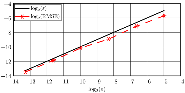
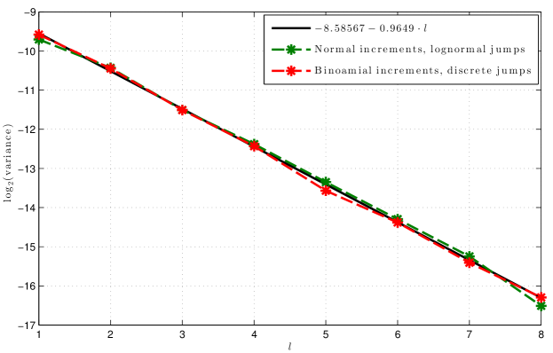
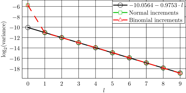
and L^=9^𝐿9\hat{L}=9. In fact in this case the exact solution is available and for above parameter values, we have E[f(XT)]0.2276799594Edelimited-[]𝑓subscript𝑋𝑇0.2276799594\mathrm{E}[f(X_{T})]\approx 0.2276799594. The variance decay is presented on Figure 5.1. In particular, the line α1α2lsubscript𝛼1subscript𝛼2𝑙\alpha_{1}-\alpha_{2}\cdot l with α2=0.9753subscript𝛼20.9753\alpha_{2}=0.9753 fits the estimated log-variances best and this is in agreement with Corollary 2. The corresponding RMSE is presented in Figure 5.2.
Refer to caption

Figure 5.1: Three dimensional European max-call option: level variances for schemes with binomial and normal increments.

Refer to caption

Figure 5.2: Three dimensional European max-call option: estimated RMSE against the required precision ε𝜀\varepsilon for different values of ε𝜀\varepsilon.

5.1.2 Geometric Asian option

Consider a one dimensional process Xt,subscript𝑋𝑡X_{t}, t[0,T],𝑡0𝑇t\in[0,T], where each coordinate process Xtisubscriptsuperscript𝑋𝑖𝑡X^{i}_{t} solves one-dimensional SDE of the form (4.1) with b(x)=rx𝑏𝑥𝑟𝑥b(x)=r\cdot x and σ(x)=σx𝜎𝑥𝜎𝑥\sigma(x)=\sigma\cdot x for some r,σ\mathbbR𝑟𝜎\mathbb𝑅r,\,\sigma\in\mathbb{R}. We are interested in computing the expectation of the functional

f(X)=erTmax(exp(1T0Tlog(Xt)𝑑t)K,0).𝑓subscript𝑋superscript𝑒𝑟𝑇1𝑇superscriptsubscript0𝑇subscript𝑋𝑡differential-d𝑡𝐾0\displaystyle f(X_{\cdot})=e^{-r\cdot T}\max\left(\exp\left(\frac{1}{T}\int\limits_{0}^{T}\log(X_{t})dt\right)-K,0\right).

The parameter values are

r=0.05,σ=0.2,T=1,K=1.formulae-sequence𝑟0.05formulae-sequence𝜎0.2formulae-sequence𝑇1𝐾1\displaystyle r=0.05,\ \sigma=0.2,\ \ T=1,\ K=1.

In this case the exact value of the expectation is given by

E[f(X)]0.05546818634.Edelimited-[]𝑓subscript𝑋0.05546818634\mathrm{E}[f(X_{\cdot})]\approx 0.05546818634.

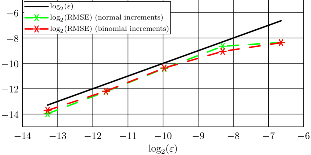
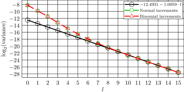
The variance decay is presented on Figure 5.3. Due the fact, that at first levels the variance decays faster than predicted, we have fitted the variance decay only on the last 6 levels with the line α1α2lsubscript𝛼1subscript𝛼2𝑙\alpha_{1}-\alpha_{2}\cdot l and got α2=1.0059subscript𝛼21.0059\alpha_{2}=1.0059. The corresponding RMSE is presented in Figure 5.4.
Refer to caption

Figure 5.3: Geometric Asian option: level log-variances for binomial and normal increments.

Refer to caption

Figure 5.4: Geometric Asian option: RMSE for binomial and normal increments.

5.2 Jump diffusions

Consider a jump SDE

dXt=(rλ(em+0.5θ21))Xtdt+σXtWt+XtdJ(t),𝑑subscript𝑋𝑡𝑟𝜆superscript𝑒𝑚0.5superscript𝜃21subscript𝑋𝑡𝑑𝑡𝜎subscript𝑋𝑡subscript𝑊𝑡subscript𝑋𝑡𝑑𝐽𝑡dX_{t}=\left(r-\lambda\cdot\left(e^{m+0.5\cdot\theta^{2}}-1\right)\right)\cdot X_{t}\cdot dt+\sigma\cdot X_{t}\cdot W_{t}+X_{t}\cdot dJ(t),

where

J(t)=j=1N(t)(Yj1),log(Yj)𝒩(m,θ2)formulae-sequence𝐽𝑡superscriptsubscript𝑗1𝑁𝑡subscript𝑌𝑗1similar-tosubscript𝑌𝑗𝒩𝑚superscript𝜃2J(t)=\sum\limits_{j=1}^{N(t)}(Y_{j}-1),\quad\log(Y_{j})\sim\mathcal{N}(m,\theta^{2})

and N(t)𝑁𝑡N(t) is a Poisson process with rate λ𝜆\lambda. We are interested in computing the expectation of

f(XT)=erTmax(X(T)K,0).𝑓subscript𝑋𝑇superscript𝑒𝑟𝑇𝑋𝑇𝐾0\displaystyle f(X_{T})=e^{-r\cdot T}\max\left(X(T)-K,0\right).

The parameters’ values are

r=0.05,σ=0.2,λ=0.5,m=0.05,θ=0.25,T=1,K=1.formulae-sequence𝑟0.05formulae-sequence𝜎0.2formulae-sequence𝜆0.5formulae-sequence𝑚0.05formulae-sequence𝜃0.25formulae-sequence𝑇1𝐾1\displaystyle r=0.05,\ \sigma=0.2,\ \lambda=0.5,\ m=0.05,\ \theta=0.25,\ T=1,\ K=1.

It follows from [9] (Section 3.5) that, for above parameter values E[f(XT)]0.153065585Edelimited-[]𝑓subscript𝑋𝑇0.153065585\mathrm{E}[f(X_{T})]\approx 0.153065585. We have performed two types of simulations with the fixed top level L^=8^𝐿8\hat{L}=8:

  • Y𝑌Y was sampled from the lognormal distribution, while the increments of the Brownian motion were modelled as normal random variables

  • Y𝑌Y was sampled as a discrete random variable Y^^𝑌\hat{Y} according to the Remark 4.8, with moments matching first 666 moments of the lognormal distribution, while the increments of the Brownian motion were modelled as discrete random variable defined by (4.4).

In both of those cases, the number of jumps ηl,jsubscript𝜂𝑙𝑗\eta_{l,j} at the level l𝑙l and step j𝑗j is generated via

ηl,jBi(2L^l,2L^λ).similar-tosubscript𝜂𝑙𝑗Bisuperscript2^𝐿𝑙superscript2^𝐿𝜆\displaystyle\eta_{l,j}\sim\mathrm{Bi}\left(2^{\hat{L}-l},2^{-\hat{L}}\cdot\lambda\right). (5.1)

One can see, that (5.1) can be implemented in the same spirit as (4.4). On the finest level L,𝐿L, we allow only for two jumps 00 or 1.11. Let us denote by μisubscript𝜇𝑖\mu_{i} the i𝑖ith moment of the lognormal distribution with parameters m𝑚m and θ𝜃\theta. The random variable Y^^𝑌\hat{Y} takes 444 values with probabilities p1,,p4subscript𝑝1subscript𝑝4p_{1},\ldots,p_{4}. The values and probabilities are obtained by solving the optimization problem:

Minimize
(k=14pkxk7μ7)2superscriptsuperscriptsubscript𝑘14subscript𝑝𝑘superscriptsubscript𝑥𝑘7subscript𝜇72\displaystyle\left(\sum_{k=1}^{4}p_{k}\cdot x_{k}^{7}-\mu_{7}\right)^{2}
Subject to
k=14pkxki=μi,i=1,,6formulae-sequencesuperscriptsubscript𝑘14subscript𝑝𝑘superscriptsubscript𝑥𝑘𝑖subscript𝜇𝑖𝑖16\displaystyle\sum_{k=1}^{4}p_{k}\cdot x_{k}^{i}=\mu_{i},\qquad i=1,\ldots,6

The solution is

p1=0.608176614910593,subscript𝑝10.608176614910593\displaystyle p_{1}=0.608176614910593, x1=1.081500568717563subscript𝑥11.081500568717563\displaystyle\quad x_{1}=1.081500568717563
p2=0.003503326771883,subscript𝑝20.003503326771883\displaystyle p_{2}=0.003503326771883, x2=2.376117006693613subscript𝑥22.376117006693613\displaystyle\quad x_{2}=2.376117006693613
p3=0.226782660300013,subscript𝑝30.226782660300013\displaystyle p_{3}=0.226782660300013, x3=0.719559222085786subscript𝑥30.719559222085786\displaystyle\quad x_{3}=0.719559222085786
p4=0.161537398017512,subscript𝑝40.161537398017512\displaystyle p_{4}=0.161537398017512, x4=1.581001071314797subscript𝑥41.581001071314797\displaystyle\quad x_{4}=1.581001071314797

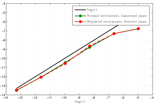
The variance decay is shown in Figure 5.5 for both types of simulations. We estimated RMSE of the ML estimate based on the weak Euler scheme based on 505050 independent runs, see Figure 5.6.

Refer to caption


Figure 5.5: European option: level log-variances for binomial increments and discrete jumps, normal increments and lognormal jumps.

Refer to caption


Figure 5.6: European option: RMSE for binomial increments and discrete jumps, normal increments and lognormal jumps.
Acknowledgments

Authors are thankful to Prof. Mike Giles, Dr. Lukasz Szpruch and Dr. Sonja Cox for their helpful comments and remarks. Authors are very grateful to Vladimir Shiryaev for his assistance with the numerical experiments.

6 Proofs

Lemma 7.

Suppose that the coefficient function a𝑎a in (1.1) is uniformly Lipschitz and has at most linear growth, i.e.,

a(x)a(x)Laxx,a(x)2Ba2(1+x2)formulae-sequencenorm𝑎𝑥𝑎superscript𝑥subscript𝐿𝑎norm𝑥superscript𝑥superscriptnorm𝑎𝑥2subscriptsuperscript𝐵2𝑎1superscriptnorm𝑥2\displaystyle\|a(x)-a(x^{\prime})\|\leq L_{a}\,\|x-x^{\prime}\|,\quad\|a(x)\|^{2}\leq B^{2}_{a}\,(1+\|x\|^{2}) (6.1)

for any x,x\mathbbRd𝑥superscript𝑥\mathbbsuperscript𝑅𝑑x,x^{\prime}\in\mathbb{R}^{d} and some positive constants Lasubscript𝐿𝑎L_{a} and Ba.subscript𝐵𝑎B_{a}. Moreover, assume that E[X02]<,Edelimited-[]superscriptnormsubscript𝑋02\mathrm{E}[\|X_{0}\|^{2}]<\infty, then the following estimates hold

E[XnΔff2]3Ba2(nmf,2+n2mf,12)exp(3Ba2(nmf,2+n2mf,12)),Edelimited-[]superscriptdelimited-∥∥superscriptsubscript𝑋𝑛subscriptΔ𝑓𝑓23superscriptsubscript𝐵𝑎2𝑛subscript𝑚𝑓2superscript𝑛2subscriptsuperscript𝑚2𝑓13superscriptsubscript𝐵𝑎2𝑛subscript𝑚𝑓2superscript𝑛2subscriptsuperscript𝑚2𝑓1\mathrm{E}\left[\bigl{\|}X_{n\Delta_{f}}^{f}\bigr{\|}^{2}\right]\leq 3B_{a}^{2}\cdot(n\cdot m_{f,2}+n^{2}\cdot m^{2}_{f,1})\cdot\exp\left(3B_{a}^{2}\cdot(n\cdot m_{f,2}+n^{2}\cdot m^{2}_{f,1})\right),
E[XnΔcc2]3Ba2(nmf,2+n2mf,12)exp(3Ba2(nmf,2+n2mf,12)),Edelimited-[]superscriptdelimited-∥∥superscriptsubscript𝑋𝑛subscriptΔ𝑐𝑐23superscriptsubscript𝐵𝑎2𝑛subscript𝑚𝑓2superscript𝑛2subscriptsuperscript𝑚2𝑓13superscriptsubscript𝐵𝑎2𝑛subscript𝑚𝑓2superscript𝑛2subscriptsuperscript𝑚2𝑓1\mathrm{E}\left[\bigl{\|}X_{n\Delta_{c}}^{c}\bigr{\|}^{2}\right]\leq 3B_{a}^{2}\cdot(n\cdot m_{f,2}+n^{2}\cdot m^{2}_{f,1})\cdot\exp\left(3B_{a}^{2}\cdot(n\cdot m_{f,2}+n^{2}\cdot m^{2}_{f,1})\right),

for n=1,,nc.𝑛1subscript𝑛𝑐n=1,\ldots,n_{c}.

Proof.

Since

XnΔffsuperscriptsubscript𝑋𝑛subscriptΔ𝑓𝑓\displaystyle X_{n\Delta_{f}}^{f} =X0+i=1n(XiΔffX(i1)Δff),absentsubscript𝑋0superscriptsubscript𝑖1𝑛superscriptsubscript𝑋𝑖subscriptΔ𝑓𝑓superscriptsubscript𝑋𝑖1subscriptΔ𝑓𝑓\displaystyle=X_{0}+\sum\limits_{i=1}^{n}\left(X_{i\Delta_{f}}^{f}-X_{(i-1)\Delta_{f}}^{f}\right),

we have, due to independence of the increments

E[XnΔff2]Edelimited-[]superscriptdelimited-∥∥superscriptsubscript𝑋𝑛subscriptΔ𝑓𝑓2\displaystyle\mathrm{E}\left[\bigl{\|}X_{n\Delta_{f}}^{f}\bigr{\|}^{2}\right] =E[X0+i=1na(X(i1)Δff)(ζifE[ζif])+i=1na(X(i1)Δff)E[ζif]2]absentEdelimited-[]superscriptdelimited-∥∥subscript𝑋0superscriptsubscript𝑖1𝑛𝑎superscriptsubscript𝑋𝑖1subscriptΔ𝑓𝑓superscriptsubscript𝜁𝑖𝑓Edelimited-[]superscriptsubscript𝜁𝑖𝑓superscriptsubscript𝑖1𝑛𝑎superscriptsubscript𝑋𝑖1subscriptΔ𝑓𝑓Edelimited-[]superscriptsubscript𝜁𝑖𝑓2\displaystyle=\mathrm{E}\left[\Bigl{\|}X_{0}+\sum\limits_{i=1}^{n}a\bigl{(}X_{(i-1)\Delta_{f}}^{f}\bigr{)}\cdot(\zeta_{i}^{f}-\mathrm{E}[\zeta_{i}^{f}]\bigr{)}+\sum\limits_{i=1}^{n}a\bigl{(}X_{(i-1)\Delta_{f}}^{f}\bigr{)}\cdot\mathrm{E}[\zeta_{i}^{f}]\Bigr{\|}^{2}\right]
3E[X02]+3i=1nE[a(X(i1)Δff)2]mf,2absent3Edelimited-[]superscriptnormsubscript𝑋023superscriptsubscript𝑖1𝑛Edelimited-[]superscriptdelimited-∥∥𝑎superscriptsubscript𝑋𝑖1subscriptΔ𝑓𝑓2subscript𝑚𝑓2\displaystyle\leq 3\,\mathrm{E}[\|X_{0}\|^{2}]+3\,\sum\limits_{i=1}^{n}\mathrm{E}\left[\bigl{\|}a\bigl{(}X_{(i-1)\Delta_{f}}^{f}\bigr{)}\bigr{\|}^{2}\right]\,m_{f,2}
+3ni=1nE[a(X(i1)Δff)2]mf,123𝑛superscriptsubscript𝑖1𝑛Edelimited-[]superscriptdelimited-∥∥𝑎superscriptsubscript𝑋𝑖1subscriptΔ𝑓𝑓2subscriptsuperscript𝑚2𝑓1\displaystyle\quad+3n\,\sum\limits_{i=1}^{n}\mathrm{E}\Bigl{[}\bigl{\|}a\bigl{(}X_{(i-1)\Delta_{f}}^{f}\bigr{)}\bigr{\|}^{2}\Bigr{]}\,m^{2}_{f,1}
3E[X02]+3Ba2mf,2(n+i=1nE[Xi1f2])absent3Edelimited-[]superscriptnormsubscript𝑋023superscriptsubscript𝐵𝑎2subscript𝑚𝑓2𝑛superscriptsubscript𝑖1𝑛Edelimited-[]superscriptdelimited-∥∥subscriptsuperscript𝑋𝑓𝑖12\displaystyle\leq 3\mathrm{E}[\|X_{0}\|^{2}]+3B_{a}^{2}\cdot m_{f,2}\cdot\Bigl{(}n+\sum\limits_{i=1}^{n}\mathrm{E}\Bigl{[}\bigl{\|}X^{f}_{i-1}\bigr{\|}^{2}\Bigr{]}\Bigr{)}
+3Ba2nmf,12(n+i=1nE[Xi1f2])3superscriptsubscript𝐵𝑎2𝑛subscriptsuperscript𝑚2𝑓1𝑛superscriptsubscript𝑖1𝑛Edelimited-[]superscriptdelimited-∥∥subscriptsuperscript𝑋𝑓𝑖12\displaystyle\quad+3B_{a}^{2}\cdot n\cdot m^{2}_{f,1}\cdot\Bigl{(}n+\sum\limits_{i=1}^{n}\mathrm{E}\Bigl{[}\bigl{\|}X^{f}_{i-1}\bigr{\|}^{2}\Bigr{]}\Bigr{)}

Using the discrete version of the Gronwall inequality (see Appendix), we get

E[XnΔff2]3Ba2(nmf,2+n2mf,12)exp(3Ba2(nmf,2+n2mf,12)).Edelimited-[]superscriptdelimited-∥∥superscriptsubscript𝑋𝑛subscriptΔ𝑓𝑓23superscriptsubscript𝐵𝑎2𝑛subscript𝑚𝑓2superscript𝑛2subscriptsuperscript𝑚2𝑓13superscriptsubscript𝐵𝑎2𝑛subscript𝑚𝑓2superscript𝑛2subscriptsuperscript𝑚2𝑓1\mathrm{E}\left[\bigl{\|}X_{n\Delta_{f}}^{f}\bigr{\|}^{2}\right]\leq 3B_{a}^{2}\cdot(n\cdot m_{f,2}+n^{2}\cdot m^{2}_{f,1})\cdot\exp\left(3B_{a}^{2}\cdot(n\cdot m_{f,2}+n^{2}\cdot m^{2}_{f,1})\right).

The second inequality of the lemma is proved in the same way. ∎

6.1 Proof of Proposition  1

Due to the Lemma 7 we have

E[XnΔff2]<A1,E[XnΔcc2]<A2formulae-sequenceEdelimited-[]superscriptdelimited-∥∥superscriptsubscript𝑋𝑛subscriptΔ𝑓𝑓2subscript𝐴1Edelimited-[]superscriptdelimited-∥∥superscriptsubscript𝑋𝑛subscriptΔ𝑐𝑐2subscript𝐴2\displaystyle\mathrm{E}\Bigl{[}\bigl{\|}X_{n\Delta_{f}}^{f}\bigr{\|}^{2}\Bigr{]}<A_{1},\quad\mathrm{E}\Bigl{[}\bigl{\|}{X}_{n\Delta_{c}}^{c}\bigr{\|}^{2}\Bigr{]}<A_{2} (6.2)

for n=1,,nc,𝑛1subscript𝑛𝑐n=1,\ldots,n_{c}, and constants A1,subscript𝐴1A_{1}, A2subscript𝐴2A_{2} not depending on n.𝑛n. We have

XrΔcfXrΔccsuperscriptsubscript𝑋𝑟subscriptΔ𝑐𝑓superscriptsubscript𝑋𝑟subscriptΔ𝑐𝑐\displaystyle X_{r\Delta_{c}}^{f}-{X}_{r\Delta_{c}}^{c} =\displaystyle= X(r1)ΔcfX(r1)Δcc+[a(X(2r1)Δff)a(X(r1)Δcc)]ζ2rf+superscriptsubscript𝑋𝑟1subscriptΔ𝑐𝑓superscriptsubscript𝑋𝑟1subscriptΔ𝑐𝑐limit-fromdelimited-[]𝑎superscriptsubscript𝑋2𝑟1subscriptΔ𝑓𝑓𝑎superscriptsubscript𝑋𝑟1subscriptΔ𝑐𝑐superscriptsubscript𝜁2𝑟𝑓\displaystyle X_{(r-1)\Delta_{c}}^{f}-{X}_{(r-1)\Delta_{c}}^{c}+\left[a(X_{(2r-1)\Delta_{f}}^{f})-a({X}_{(r-1)\Delta_{c}}^{c})\right]\zeta_{2r}^{f}+
+[a(X(r1)Δcf)a(X(r1)Δcc)]ζ2r1fa(X(r1)Δcc)[ζrcζ2rfζ2r1f]delimited-[]𝑎superscriptsubscript𝑋𝑟1subscriptΔ𝑐𝑓𝑎superscriptsubscript𝑋𝑟1subscriptΔ𝑐𝑐superscriptsubscript𝜁2𝑟1𝑓𝑎superscriptsubscript𝑋𝑟1subscriptΔ𝑐𝑐delimited-[]superscriptsubscript𝜁𝑟𝑐superscriptsubscript𝜁2𝑟𝑓superscriptsubscript𝜁2𝑟1𝑓\displaystyle+\left[a(X_{(r-1)\Delta_{c}}^{f})-a({X}_{(r-1)\Delta_{c}}^{c})\right]\zeta_{2r-1}^{f}-a(X_{(r-1)\Delta_{c}}^{c})\left[{\zeta}_{r}^{c}-\zeta_{2r}^{f}-\zeta_{2r-1}^{f}\right]

Denote DrXrΔcfXrΔcc,approaches-limitsubscript𝐷𝑟superscriptsubscript𝑋𝑟subscriptΔ𝑐𝑓superscriptsubscript𝑋𝑟subscriptΔ𝑐𝑐D_{r}\doteq X_{r\Delta_{c}}^{f}-{X}_{r\Delta_{c}}^{c}, then we have the representation

Dr=Dr1+δr+εrsubscript𝐷𝑟subscript𝐷𝑟1subscript𝛿𝑟subscript𝜀𝑟D_{r}=D_{r-1}+\delta_{r}+\varepsilon_{r}

with

εrsubscript𝜀𝑟\displaystyle\varepsilon_{r} =\displaystyle= [a(X(2r1)Δff)a(X(r1)Δcc)](ζ2rfE[ζ2rf])delimited-[]𝑎superscriptsubscript𝑋2𝑟1subscriptΔ𝑓𝑓𝑎superscriptsubscript𝑋𝑟1subscriptΔ𝑐𝑐superscriptsubscript𝜁2𝑟𝑓Edelimited-[]superscriptsubscript𝜁2𝑟𝑓\displaystyle\left[a(X_{(2r-1)\Delta_{f}}^{f})-a({X}_{(r-1)\Delta_{c}}^{c})\right]\left(\zeta_{2r}^{f}-\mathrm{E}\bigl{[}\zeta_{2r}^{f}\bigr{]}\right)
+[a(X(r1)Δcf)a(X(r1)Δcc)](ζ2r1fE[ζ2r1f])delimited-[]𝑎superscriptsubscript𝑋𝑟1subscriptΔ𝑐𝑓𝑎superscriptsubscript𝑋𝑟1subscriptΔ𝑐𝑐superscriptsubscript𝜁2𝑟1𝑓Edelimited-[]superscriptsubscript𝜁2𝑟1𝑓\displaystyle+\left[a(X_{(r-1)\Delta_{c}}^{f})-a({X}_{(r-1)\Delta_{c}}^{c})\right]\left(\zeta_{2r-1}^{f}-\mathrm{E}\bigl{[}\zeta_{2r-1}^{f}\bigr{]}\right)
a(X(r1)Δcc)[ζrcζ2rfζ2r1f]𝑎superscriptsubscript𝑋𝑟1subscriptΔ𝑐𝑐delimited-[]superscriptsubscript𝜁𝑟𝑐superscriptsubscript𝜁2𝑟𝑓superscriptsubscript𝜁2𝑟1𝑓\displaystyle-a({X}_{(r-1)\Delta_{c}}^{c})\left[{\zeta}_{r}^{c}-\zeta_{2r}^{f}-\zeta_{2r-1}^{f}\right]

and

δrsubscript𝛿𝑟\displaystyle\delta_{r} =\displaystyle= [a(X(2r1)Δff)a(X(r1)Δcc)]E[ζ2rf]+[a(X(r1)Δcf)a(X(r1)Δcc)]E[ζ2r1f].delimited-[]𝑎superscriptsubscript𝑋2𝑟1subscriptΔ𝑓𝑓𝑎superscriptsubscript𝑋𝑟1subscriptΔ𝑐𝑐Edelimited-[]superscriptsubscript𝜁2𝑟𝑓delimited-[]𝑎superscriptsubscript𝑋𝑟1subscriptΔ𝑐𝑓𝑎superscriptsubscript𝑋𝑟1subscriptΔ𝑐𝑐Edelimited-[]superscriptsubscript𝜁2𝑟1𝑓\displaystyle\left[a(X_{(2r-1)\Delta_{f}}^{f})-a({X}_{(r-1)\Delta_{c}}^{c})\right]\mathrm{E}\bigl{[}\zeta_{2r}^{f}\bigr{]}+\left[a(X_{(r-1)\Delta_{c}}^{f})-a({X}_{(r-1)\Delta_{c}}^{c})\right]\mathrm{E}\bigl{[}\zeta_{2r-1}^{f}\bigr{]}.

The Lipschitz continuity of the function a𝑎a implies

E[a(X(2r1)Δff)a(X(r1)Δcc)2]Edelimited-[]superscriptdelimited-∥∥𝑎superscriptsubscript𝑋2𝑟1subscriptΔ𝑓𝑓𝑎superscriptsubscript𝑋𝑟1subscriptΔ𝑐𝑐2\displaystyle\mathrm{E}\left[\bigl{\|}a(X_{(2r-1)\Delta_{f}}^{f})-a({X}_{(r-1)\Delta_{c}}^{c})\bigr{\|}^{2}\right] \displaystyle\leq La2E[X(2r1)ΔffX(r1)Δcc2]superscriptsubscript𝐿𝑎2Edelimited-[]superscriptdelimited-∥∥superscriptsubscript𝑋2𝑟1subscriptΔ𝑓𝑓superscriptsubscript𝑋𝑟1subscriptΔ𝑐𝑐2\displaystyle L_{a}^{2}\,\mathrm{E}\left[\bigl{\|}X_{(2r-1)\Delta_{f}}^{f}-{X}_{(r-1)\Delta_{c}}^{c}\bigr{\|}^{2}\right]
\displaystyle\leq 2La2E[Dr12]2superscriptsubscript𝐿𝑎2Edelimited-[]superscriptdelimited-∥∥subscript𝐷𝑟12\displaystyle 2\,L_{a}^{2}\,\mathrm{E}\left[\bigl{\|}D_{r-1}\bigr{\|}^{2}\right]
+2La2Ba2(1+EX(r1)Δcf2)E[ζ2r1f2]2superscriptsubscript𝐿𝑎2superscriptsubscript𝐵𝑎21Esuperscriptdelimited-∥∥superscriptsubscript𝑋𝑟1subscriptΔ𝑐𝑓2Edelimited-[]superscriptdelimited-∥∥superscriptsubscript𝜁2𝑟1𝑓2\displaystyle+2\,L_{a}^{2}\,B_{a}^{2}\,\left(1+\mathrm{E}\bigl{\|}X_{(r-1)\Delta_{c}}^{f}\bigr{\|}^{2}\right)\mathrm{E}\left[\bigl{\|}\zeta_{2r-1}^{f}\bigr{\|}^{2}\right]

and

E[a(X(r1)Δcf)a(X(r1)Δcc)2]La2E[Dr12].Edelimited-[]superscriptdelimited-∥∥𝑎superscriptsubscript𝑋𝑟1subscriptΔ𝑐𝑓𝑎superscriptsubscript𝑋𝑟1subscriptΔ𝑐𝑐2superscriptsubscript𝐿𝑎2Edelimited-[]superscriptdelimited-∥∥subscript𝐷𝑟12\mathrm{E}\left[\bigl{\|}a(X_{(r-1)\Delta_{c}}^{f})-a({X}_{(r-1)\Delta_{c}}^{c})\bigr{\|}^{2}\right]\leq L_{a}^{2}\,\mathrm{E}\left[\bigl{\|}D_{r-1}\bigr{\|}^{2}\right].

As a result

E[εr2]Edelimited-[]superscriptdelimited-∥∥subscript𝜀𝑟2\displaystyle\mathrm{E}\left[\bigl{\|}\varepsilon_{r}\bigr{\|}^{2}\right] \displaystyle\leq 3E[a(X(2r1)Δff)a(X(r1)Δcc)2]E[ξ2rf2]+limit-from3Edelimited-[]superscriptdelimited-∥∥𝑎superscriptsubscript𝑋2𝑟1subscriptΔ𝑓𝑓𝑎superscriptsubscript𝑋𝑟1subscriptΔ𝑐𝑐2Edelimited-[]superscriptdelimited-∥∥superscriptsubscript𝜉2𝑟𝑓2\displaystyle 3\mathrm{E}\left[\bigl{\|}a(X_{(2r-1)\Delta_{f}}^{f})-a({X}_{(r-1)\Delta_{c}}^{c})\bigr{\|}^{2}\right]\mathrm{E}\left[\bigl{\|}\xi_{2r}^{f}\bigr{\|}^{2}\right]+
+3E[a(X(r1)Δcf)a(X(r1)Δcc)2]E[ξ2r1f2]3Edelimited-[]superscriptdelimited-∥∥𝑎superscriptsubscript𝑋𝑟1subscriptΔ𝑐𝑓𝑎superscriptsubscript𝑋𝑟1subscriptΔ𝑐𝑐2Edelimited-[]superscriptdelimited-∥∥superscriptsubscript𝜉2𝑟1𝑓2\displaystyle+3\mathrm{E}\left[\bigl{\|}a(X_{(r-1)\Delta_{c}}^{f})-a({X}_{(r-1)\Delta_{c}}^{c})\bigr{\|}^{2}\right]\mathrm{E}\left[\bigl{\|}\xi_{2r-1}^{f}\bigr{\|}^{2}\right]
+3E[a(X(r1)Δcc)2]E[ζrcζ2rfζ2r1f2]3Edelimited-[]superscriptdelimited-∥∥𝑎superscriptsubscript𝑋𝑟1subscriptΔ𝑐𝑐2Edelimited-[]superscriptdelimited-∥∥superscriptsubscript𝜁𝑟𝑐superscriptsubscript𝜁2𝑟𝑓superscriptsubscript𝜁2𝑟1𝑓2\displaystyle+3\mathrm{E}\left[\bigl{\|}a({X}_{(r-1)\Delta_{c}}^{c})\bigr{\|}^{2}\right]\mathrm{E}\left[\bigl{\|}{\zeta}_{r}^{c}-\zeta_{2r}^{f}-\zeta_{2r-1}^{f}\bigr{\|}^{2}\right]
\displaystyle\leq c1(1+EX(r1)Δcf2)E[ξ2r1f2]E[ξ2rf2]+limit-fromsubscript𝑐11Esuperscriptdelimited-∥∥superscriptsubscript𝑋𝑟1subscriptΔ𝑐𝑓2Edelimited-[]superscriptdelimited-∥∥superscriptsubscript𝜉2𝑟1𝑓2Edelimited-[]superscriptdelimited-∥∥superscriptsubscript𝜉2𝑟𝑓2\displaystyle c_{1}\left(1+\mathrm{E}\bigl{\|}X_{(r-1)\Delta_{c}}^{f}\bigr{\|}^{2}\right)\mathrm{E}\left[\bigl{\|}\xi_{2r-1}^{f}\bigr{\|}^{2}\right]\mathrm{E}\left[\bigl{\|}\xi_{2r}^{f}\bigr{\|}^{2}\right]+
+c2E[Dr12](E[ξ2rf2]+E[ξ2r1f2])subscript𝑐2Edelimited-[]superscriptdelimited-∥∥subscript𝐷𝑟12Edelimited-[]superscriptdelimited-∥∥superscriptsubscript𝜉2𝑟𝑓2Edelimited-[]superscriptdelimited-∥∥superscriptsubscript𝜉2𝑟1𝑓2\displaystyle+c_{2}\mathrm{E}\left[\bigl{\|}D_{r-1}\bigr{\|}^{2}\right]\left(\mathrm{E}\left[\bigl{\|}\xi_{2r}^{f}\bigr{\|}^{2}\right]+\mathrm{E}\left[\bigl{\|}\xi_{2r-1}^{f}\bigr{\|}^{2}\right]\right)
+c3(1+E[X(r1)Δcc2])subscript𝑐31Edelimited-[]superscriptdelimited-∥∥superscriptsubscript𝑋𝑟1subscriptΔ𝑐𝑐2\displaystyle+c_{3}\left(1+\mathrm{E}\left[\bigl{\|}X_{(r-1)\Delta_{c}}^{c}\bigr{\|}^{2}\right]\right)\mathcal{R}
\displaystyle\leq c4[mf,2E[Dr12]+mf,22+]subscript𝑐4delimited-[]subscript𝑚𝑓2Edelimited-[]superscriptdelimited-∥∥subscript𝐷𝑟12superscriptsubscript𝑚𝑓22\displaystyle c_{4}\left[m_{f,2}\mathrm{E}\left[\bigl{\|}D_{r-1}\bigr{\|}^{2}\right]+m_{f,2}^{2}+\mathcal{R}\right]

for some constants c1,c2,subscript𝑐1subscript𝑐2c_{1},c_{2}, c3,subscript𝑐3c_{3}, c4subscript𝑐4c_{4} and E[ζrcζ2rf+ζ2r1f2].approaches-limitEdelimited-[]superscriptdelimited-∥∥superscriptsubscript𝜁𝑟𝑐superscriptsubscript𝜁2𝑟𝑓superscriptsubscript𝜁2𝑟1𝑓2\mathcal{R}\doteq\mathrm{E}\left[\bigl{\|}{\zeta}_{r}^{c}-\zeta_{2r}^{f}+\zeta_{2r-1}^{f}\bigr{\|}^{2}\right]. Analogously

E[δr2]c5[mf,12E[Dr12]+mf,12mf,2]Edelimited-[]superscriptdelimited-∥∥subscript𝛿𝑟2subscript𝑐5delimited-[]superscriptsubscript𝑚𝑓12Edelimited-[]superscriptdelimited-∥∥subscript𝐷𝑟12superscriptsubscript𝑚𝑓12subscript𝑚𝑓2\mathrm{E}\left[\bigl{\|}\delta_{r}\bigr{\|}^{2}\right]\leq c_{5}\left[m_{f,1}^{2}\mathrm{E}\left[\bigl{\|}D_{r-1}\bigr{\|}^{2}\right]+m_{f,1}^{2}m_{f,2}\right]

for some c5>0.subscript𝑐50c_{5}>0. Define

Mr=j=1rεjsubscript𝑀𝑟superscriptsubscript𝑗1𝑟subscript𝜀𝑗M_{r}=\sum_{j=1}^{r}\varepsilon_{j}

and note that Mrsubscript𝑀𝑟M_{r} is martingale with respect to the filtration

rσ(X(2j1)Δff,X(j1)Δcc,X(j1)Δcf,jr),r=1,,nc+1.formulae-sequenceapproaches-limitsubscript𝑟𝜎superscriptsubscript𝑋2𝑗1subscriptΔ𝑓𝑓superscriptsubscript𝑋𝑗1subscriptΔ𝑐𝑐superscriptsubscript𝑋𝑗1subscriptΔ𝑐𝑓𝑗𝑟𝑟1subscript𝑛𝑐1\mathcal{F}_{r}\doteq\sigma\left(X_{(2j-1)\Delta_{f}}^{f},{X}_{(j-1)\Delta_{c}}^{c},X_{(j-1)\Delta_{c}}^{f},\,j\leq r\right),\quad r=1,\ldots,n_{c}+1.

Hence the Doob inequality implies for any nnc::𝑛subscript𝑛𝑐absentn\leq n_{c}:

E[supr=1,,nMr2]Edelimited-[]superscriptdelimited-∥∥subscriptsupremum𝑟1𝑛subscript𝑀𝑟2\displaystyle\mathrm{E}\left[\bigl{\|}\sup_{r=1,\ldots,n}M_{r}\bigr{\|}^{2}\right] \displaystyle\leq E[Mn2]Edelimited-[]superscriptdelimited-∥∥subscript𝑀𝑛2\displaystyle\mathrm{E}\left[\bigl{\|}M_{n}\bigr{\|}^{2}\right]
\displaystyle\leq c6mf,2j=1nE[Dj12]+c6nmf,22+c6n.subscript𝑐6subscript𝑚𝑓2superscriptsubscript𝑗1𝑛Edelimited-[]superscriptdelimited-∥∥subscript𝐷𝑗12subscript𝑐6𝑛superscriptsubscript𝑚𝑓22subscript𝑐6𝑛\displaystyle c_{6}m_{f,2}\sum_{j=1}^{n}\mathrm{E}\left[\bigl{\|}D_{j-1}\bigr{\|}^{2}\right]+c_{6}nm_{f,2}^{2}+c_{6}n\,\mathcal{R}.

So we have for D¯nmaxj=1,,nDjapproaches-limitsubscript¯𝐷𝑛subscript𝑗1𝑛subscript𝐷𝑗\overline{D}_{n}\doteq\max_{j=1,\ldots,n}D_{j}

E[D¯n2]Edelimited-[]superscriptdelimited-∥∥subscript¯𝐷𝑛2\displaystyle\mathrm{E}\left[\bigl{\|}\overline{D}_{n}\bigr{\|}^{2}\right] \displaystyle\leq 2nj=1nE[δj2]+2E[Mn2]2𝑛superscriptsubscript𝑗1𝑛Edelimited-[]superscriptdelimited-∥∥subscript𝛿𝑗22Edelimited-[]superscriptdelimited-∥∥subscript𝑀𝑛2\displaystyle 2\cdot n\sum_{j=1}^{n}\mathrm{E}\left[\bigl{\|}\delta_{j}\bigr{\|}^{2}\right]+2\cdot\mathrm{E}\left[\bigl{\|}M_{n}\bigr{\|}^{2}\right]
\displaystyle\leq c7(mf,2+nmf,12)j=1nE[D¯j12]+c7n(mf,22+nmf,12mf,2+)subscript𝑐7subscript𝑚𝑓2𝑛superscriptsubscript𝑚𝑓12superscriptsubscript𝑗1𝑛Edelimited-[]superscriptdelimited-∥∥subscript¯𝐷𝑗12subscript𝑐7𝑛superscriptsubscript𝑚𝑓22𝑛superscriptsubscript𝑚𝑓12subscript𝑚𝑓2\displaystyle c_{7}\left(m_{f,2}+nm_{f,1}^{2}\right)\sum_{j=1}^{n}\mathrm{E}\left[\bigl{\|}\overline{D}_{j-1}\bigr{\|}^{2}\right]+c_{7}n\left(m_{f,2}^{2}+nm_{f,1}^{2}m_{f,2}+\mathcal{R}\right)

Finally a discrete version of Gronwall lemma (see Appendix) implies

E[D¯n2]c8n(mf,22+mf,12mf,2+)exp(c7(nmf,2+n2mf,12)).Edelimited-[]superscriptdelimited-∥∥subscript¯𝐷𝑛2subscript𝑐8𝑛superscriptsubscript𝑚𝑓22superscriptsubscript𝑚𝑓12subscript𝑚𝑓2subscript𝑐7𝑛subscript𝑚𝑓2superscript𝑛2superscriptsubscript𝑚𝑓12\mathrm{E}\left[\bigl{\|}\overline{D}_{n}\bigr{\|}^{2}\right]\leq c_{8}n\left(m_{f,2}^{2}+m_{f,1}^{2}m_{f,2}+\mathcal{R}\right)\exp\left(c_{7}\left(nm_{f,2}+n^{2}m_{f,1}^{2}\right)\right).

6.2 Proof of Proposition 6

We aim to minimize

l=0LNl(δlα+Δl1)superscriptsubscript𝑙0𝐿subscript𝑁𝑙superscriptsubscript𝛿𝑙𝛼superscriptsubscriptΔ𝑙1\sum_{l=0}^{L}N_{l}\cdot(\delta_{l}^{-\alpha}+\Delta_{l}^{-1})

subject to

min(ΔL,δL3α)ε,l=0LΔlNlε2.formulae-sequencesubscriptΔ𝐿superscriptsubscript𝛿𝐿3𝛼𝜀superscriptsubscript𝑙0𝐿subscriptΔ𝑙subscript𝑁𝑙superscript𝜀2\min(\Delta_{L},\,\delta_{L}^{3-\alpha})\leq\varepsilon,\quad\sum_{l=0}^{L}\frac{\Delta_{l}}{N_{l}}\leq\varepsilon^{2}.

We denote

al=(δlα+Δl1),l=0,,L.formulae-sequencesubscript𝑎𝑙superscriptsubscript𝛿𝑙𝛼superscriptsubscriptΔ𝑙1𝑙0𝐿a_{l}=(\delta_{l}^{-\alpha}+\Delta_{l}^{-1}),\quad l=0,\ldots,L.

From Lagrange principle we get

al=λNl2ΔlNl=(λ)Δlal1subscript𝑎𝑙𝜆superscriptsubscript𝑁𝑙2subscriptΔ𝑙subscript𝑁𝑙𝜆subscriptΔ𝑙superscriptsubscript𝑎𝑙1absent\displaystyle a_{l}=-\lambda\cdot N_{l}^{-2}\cdot\Delta_{l}\ \Rightarrow\ N_{l}=\sqrt{(-\lambda)\cdot\Delta_{l}\cdot a_{l}^{-1}}\ \Rightarrow\
l=0LΔlNl=1λl=0LΔlΔlal1=ε2λ=ε2l=0LΔlalsuperscriptsubscript𝑙0𝐿subscriptΔ𝑙subscript𝑁𝑙1𝜆superscriptsubscript𝑙0𝐿subscriptΔ𝑙subscriptΔ𝑙superscriptsubscript𝑎𝑙1superscript𝜀2𝜆superscript𝜀2superscriptsubscript𝑙0𝐿subscriptΔ𝑙subscript𝑎𝑙absent\displaystyle\sum_{l=0}^{L}\frac{\Delta_{l}}{N_{l}}=\frac{1}{\sqrt{-\lambda}}\cdot\sum_{l=0}^{L}\frac{\Delta_{l}}{\sqrt{\Delta_{l}\cdot a_{l}^{-1}}}=\varepsilon^{2}\ \Rightarrow\ \sqrt{-\lambda}=\varepsilon^{-2}\cdot\sum_{l=0}^{L}\sqrt{\Delta_{l}\cdot a_{l}}\ \Rightarrow
Nl=Δlal1ε2l=0LΔlalsubscript𝑁𝑙subscriptΔ𝑙superscriptsubscript𝑎𝑙1superscript𝜀2superscriptsubscript𝑙0𝐿subscriptΔ𝑙subscript𝑎𝑙\displaystyle N_{l}=\sqrt{\Delta_{l}\cdot a_{l}^{-1}}\cdot\varepsilon^{-2}\cdot\sum_{l=0}^{L}\sqrt{\Delta_{l}\cdot a_{l}}

So the cost has the representation

l=0LNlalsuperscriptsubscript𝑙0𝐿subscript𝑁𝑙subscript𝑎𝑙\displaystyle\sum_{l=0}^{L}N_{l}\cdot a_{l} =l=0LalΔlal1ε2k=0LΔkakabsentsuperscriptsubscript𝑙0𝐿subscript𝑎𝑙subscriptΔ𝑙superscriptsubscript𝑎𝑙1superscript𝜀2superscriptsubscript𝑘0𝐿subscriptΔ𝑘subscript𝑎𝑘\displaystyle=\sum_{l=0}^{L}a_{l}\cdot\sqrt{\Delta_{l}\cdot a_{l}^{-1}}\cdot\varepsilon^{-2}\cdot\sum_{k=0}^{L}\sqrt{\Delta_{k}\cdot a_{k}}
=ε2(l=0LΔlal)2absentsuperscript𝜀2superscriptsuperscriptsubscript𝑙0𝐿subscriptΔ𝑙subscript𝑎𝑙2\displaystyle=\varepsilon^{-2}\cdot\left(\sum_{l=0}^{L}\sqrt{\Delta_{l}\cdot a_{l}}\right)^{2}
=ε2(l=0L1+Δlδlα)2absentsuperscript𝜀2superscriptsuperscriptsubscript𝑙0𝐿1subscriptΔ𝑙superscriptsubscript𝛿𝑙𝛼2\displaystyle=\varepsilon^{-2}\cdot\left(\sum_{l=0}^{L}\sqrt{1+\frac{\Delta_{l}}{\delta_{l}^{\alpha}}}\right)^{2}

According to the restrictions on the bias we have

ΔL=ML=ε,δL=ε13α=ΔL13α.formulae-sequencesubscriptΔ𝐿superscript𝑀𝐿𝜀subscript𝛿𝐿superscript𝜀13𝛼superscriptsubscriptΔ𝐿13𝛼\Delta_{L}=M^{-L}=\varepsilon,\ \delta_{L}=\varepsilon^{\frac{1}{3-\alpha}}=\Delta_{L}^{\frac{1}{3-\alpha}}.

We now consider two cases.

  1. 1.

    We set δl=ε13αsubscript𝛿𝑙superscript𝜀13𝛼\delta_{l}=\varepsilon^{\frac{1}{3-\alpha}} constant on all the levels. Then the cost is bounded from above by

    l=0LNl(δlα+Δl1)ε2εα3α=ε6α3αprecedes-or-equalssuperscriptsubscript𝑙0𝐿subscript𝑁𝑙superscriptsubscript𝛿𝑙𝛼superscriptsubscriptΔ𝑙1superscript𝜀2superscript𝜀𝛼3𝛼superscript𝜀6𝛼3𝛼\sum_{l=0}^{L}N_{l}\cdot(\delta_{l}^{-\alpha}+\Delta_{l}^{-1})\preceq\varepsilon^{-2}\cdot\varepsilon^{-\frac{\alpha}{3-\alpha}}=\varepsilon^{-\frac{6-\alpha}{3-\alpha}}
  2. 2.

    In the second case we will set

    δl=Δl12α.subscript𝛿𝑙superscriptsubscriptΔ𝑙12𝛼\delta_{l}=\Delta_{l}^{\frac{1}{2-\alpha}}.

    Note, that δL=ΔL12α<ΔL13αsubscript𝛿𝐿superscriptsubscriptΔ𝐿12𝛼superscriptsubscriptΔ𝐿13𝛼\delta_{L}=\Delta_{L}^{\frac{1}{2-\alpha}}<\Delta_{L}^{\frac{1}{3-\alpha}}, so the bias condition is fulfilled. Then the overall cost

    ε2(l=0L1+Δlδlα)2superscript𝜀2superscriptsuperscriptsubscript𝑙0𝐿1subscriptΔ𝑙superscriptsubscript𝛿𝑙𝛼2\displaystyle\varepsilon^{-2}\cdot\left(\sum_{l=0}^{L}\sqrt{1+\frac{\Delta_{l}}{\delta_{l}^{\alpha}}}\right)^{2} ε2(l=0L1+Δl1α2α)2asymptotically-equalsabsentsuperscript𝜀2superscriptsuperscriptsubscript𝑙0𝐿1superscriptsubscriptΔ𝑙1𝛼2𝛼2\displaystyle\asymp\varepsilon^{-2}\cdot\left(\sum_{l=0}^{L}\sqrt{1+\Delta_{l}^{1-\frac{\alpha}{2-\alpha}}}\right)^{2}
    ε2(l=0L1+Δl22α2α)2.asymptotically-equalsabsentsuperscript𝜀2superscriptsuperscriptsubscript𝑙0𝐿1superscriptsubscriptΔ𝑙22𝛼2𝛼2\displaystyle\asymp\varepsilon^{-2}\cdot\left(\sum_{l=0}^{L}\sqrt{1+\Delta_{l}^{\frac{2-2\cdot\alpha}{2-\alpha}}}\right)^{2}.

Combining all the cases together we get the statement.

7 Appendix

Lemma 8.

Let (yn)subscript𝑦𝑛(y_{n}) and (gn)subscript𝑔𝑛(g_{n}) be two nonnegative sequences and let c𝑐c be a nonnegative constant. If

ync+k=1ngkyk,n0,formulae-sequencesubscript𝑦𝑛𝑐superscriptsubscript𝑘1𝑛subscript𝑔𝑘subscript𝑦𝑘𝑛0\displaystyle y_{n}\leq c+\sum_{k=1}^{n}g_{k}y_{k},\quad n\geq 0,

then

yncexp(k=1ngk).subscript𝑦𝑛𝑐superscriptsubscript𝑘1𝑛subscript𝑔𝑘\displaystyle y_{n}\leq c\exp\left(\sum_{k=1}^{n}g_{k}\right).
Proof.

We have

ynsubscript𝑦𝑛\displaystyle y_{n} \displaystyle\leq c+0k<ncgkk<j<n(1+gj)𝑐subscript0𝑘𝑛𝑐subscript𝑔𝑘subscriptproduct𝑘𝑗𝑛1subscript𝑔𝑗\displaystyle c+\sum_{0\leq k<n}cg_{k}\prod_{k<j<n}(1+g_{j})
=\displaystyle= c+c0k<n[kj<n(1+gj)k+1j<n(1+gj)]𝑐𝑐subscript0𝑘𝑛delimited-[]subscriptproduct𝑘𝑗𝑛1subscript𝑔𝑗subscriptproduct𝑘1𝑗𝑛1subscript𝑔𝑗\displaystyle c+c\sum_{0\leq k<n}\left[\prod_{k\leq j<n}(1+g_{j})-\prod_{k+1\leq j<n}(1+g_{j})\right]
=\displaystyle= c+c[0j<n(1+gj)n+1j<n(1+gj)]𝑐𝑐delimited-[]subscriptproduct0𝑗𝑛1subscript𝑔𝑗subscriptproduct𝑛1𝑗𝑛1subscript𝑔𝑗\displaystyle c+c\left[\prod_{0\leq j<n}(1+g_{j})-\prod_{n+1\leq j<n}(1+g_{j})\right]
=\displaystyle= c0j<n(1+gj)𝑐subscriptproduct0𝑗𝑛1subscript𝑔𝑗\displaystyle c\prod_{0\leq j<n}(1+g_{j})
\displaystyle\leq cexp(0j<ngj).𝑐subscript0𝑗𝑛subscript𝑔𝑗\displaystyle c\exp\left(\sum_{0\leq j<n}g_{j}\right).

References

  • [1] Søren Asmussen and Jan Rosiński. Approximations of small jumps of Lévy processes with a view towards simulation. Journal of Applied Probability, pages 482–493, 2001.
  • [2] Vlad Bally and Denis Talay. The Euler scheme for stochastic differential equations: error analysis with Malliavin calculus. Mathematics and computers in simulation, 38(1):35–41, 1995.
  • [3] Steffen Dereich et al. Multilevel Monte Carlo algorithms for Lévy-driven sdes with gaussian correction. The Annals of Applied Probability, 21(1):283–311, 2011.
  • [4] Luc Devroye. Non-uniform random variate generation. Springer-Verlag, 1986.
  • [5] El Hadj Aly Dia et al. Error bounds for small jumps of Lévy processes. Advances in Applied Probability, 45(1):86–105, 2013.
  • [6] Nicolas Fournier. Simulation and approximation of Lévy-driven stochastic differential equations. ESAIM: Probability and Statistics, 15:233–248, 2011.
  • [7] Michael B Giles. Multilevel Monte Carlo path simulation. Operations Research, 56(3):607–617, 2008.
  • [8] Mike Giles and Yuan Xia. Multilevel Monte Carlo for exponential L\\\backslash{{\{e}}\} vy models. arXiv preprint arXiv:1403.5309, 2014.
  • [9] Paul Glasserman. Monte Carlo methods in financial engineering, volume 53. Springer, 2004.
  • [10] Jean Jacod, Thomas G Kurtz, Sylvie Méléard, and Philip Protter. The approximate euler method for Lévy driven stochastic differential equations. Annales de l’Institut Henri Poincare (B) Probability and Statistics, 41(3):523–558, 2005.
  • [11] Benjamin Jourdain and Arturo Kohatsu-Higa. A review of recent results on approximation of solutions of stochastic differential equations. In Stochastic Analysis with Financial Applications, pages 121–144. Springer, 2011.
  • [12] Shigeo Kusuoka. Approximation of expectation of diffusion processes based on Lie algebra and Malliavin calculus. In Advances in mathematical economics, pages 69–83. Springer, 2004.
  • [13] Terry Lyons and Nicolas Victoir. Cubature on Wiener space. Proceedings of the Royal Society of London. Series A: Mathematical, Physical and Engineering Sciences, 460(2041):169–198, 2004.
  • [14] Mariko Ninomiya and Syoiti Ninomiya. A new higher-order weak approximation scheme for stochastic differential equations and the Runge–Kutta method. Finance and Stochastics, 13(3):415–443, 2009.
  • [15] Syoiti Ninomiya and Nicolas Victoir. Weak approximation of stochastic differential equations and application to derivative pricing. Applied Mathematical Finance, 15(2):107–121, 2008.
  • [16] Eckhard Platen and Nicola Bruti-Liberati. Numerical solution of stochastic differential equations with jumps in finance, volume 64. Springer, 2010.
  • [17] Philip Protter, Denis Talay, et al. The euler scheme for Lévy driven stochastic differential equations. The Annals of Probability, 25(1):393–423, 1997.
  • [18] Sylvain Rubenthaler. Numerical simulation of the solution of a stochastic differential equation driven by a Lévy process. Stochastic processes and their applications, 103(2):311–349, 2003.
  • [19] Denis Talay and Luciano Tubaro. Expansion of the global error for numerical schemes solving stochastic differential equations. Stochastic analysis and applications, 8(4):483–509, 1990.
  • [20] Hideyuki Tanaka, Arturo Kohatsu-Higa, et al. An operator approach for Markov chain weak approximations with an application to infinite activity Lévy driven sdes. The Annals of Applied Probability, 19(3):1026–1062, 2009.
  • [21] Shinzo Watanabe and Nobuyuki Ikeda. Stochastic differential equations and diffusion processes. Elsevier, 1981.