Faithful Glitch Propagation in Binary Circuit Models

Abstract

Modern digital circuit design relies on fast digital timing simulation tools and, hence, on accurate binary-valued circuit models that faithfully model signal propagation, even throughout a complex design. Of particular importance is the ability to trace glitches and other short pulses, as their presence/absence may even affect a circuit’s correctness. Unfortunately, it was recently proved [Függer et al., ASYNC’13] that no existing binary-valued circuit model proposed so far, including the two most commonly used pure and inertial delay channels, faithfully captures glitch propagation: For the simple Short-Pulse Filtration (SPF) problem, which is related to a circuit’s ability to suppress a single glitch, we showed that the quite broad class of bounded single-history channels either contradict the unsolvability of SPF in bounded time or the solvability of SPF in unbounded time in physical circuits.

In this paper, we propose a class of binary circuit models that do not suffer from this deficiency: Like bounded single-history channels, our involution channels involve delays that may depend on the time of the previous output transition. Their characteristic property are delay functions which are based on involutions, i.e., functions that form their own inverse. A concrete example of such a delay function, which is derived from a generalized first-order analog circuit model, reveals that this is not an unrealistic assumption. We prove that, in sharp contrast to what is possible with bounded single-history channels, SPF cannot be solved in bounded time due to the nonexistence of a lower bound on the delay of involution channels, whereas it is easy to provide an unbounded SPF implementation. It hence follows that binary-valued circuit models based on involution channels allow to solve SPF precisely when this is possible in physical circuits. To the best of our knowledge, our model is hence the very first candidate for a model that indeed guarantees faithful glitch propagation.

1 Introduction

The steadily increasing complexity of digital circuit designs in conjunction with the large simulation times of accurate analog simulations fuel the need for analysis techniques that are (i) fast and sufficiently accurate, and (ii) ideally also facilitate a formal analysis of circuit parameters/correctness at a sufficiently high level of abstraction. Whereas there is a considerable body of work on timing analysis of circuits based on approximating the involved differential equations [NP73:spice, Ho84:thesis, LM84, PR90, DS90], these approaches still suffer from large simulation times and high memory consumption.

Popular VHDL or Verilog simulators hence employ digital timing simulations, based on continuous-time, discrete-value, rather than analog-value, circuit models. Their modeling accuracy crucially depends on the ability to accurately predict the propagation of signal transitions throughout a circuit. More specifically, precise timing models are not only important for accurate performance and power consumption estimates at early design stages, but also for assessing a circuit’s correctness: Bi-stable elements like latches, flip-flops, and arbiters fail to work correctly when glitches or signal transitions occur at improper times, and may cause metastability (including high-frequency pulse trains due to oscillatory metastability) [Mar81] on that occasion. Since such phenomenons cannot simply be assumed to have vanished at the occurrence of the next clock transition or the next handshake signal in today’s high-speed circuits, the accurate prediction of the presence/absence of glitches and similar short pulses is crucial.

Binary value, continuous time circuit models based on pure and inertial delay channels [Ung71] have been introduced several decades ago, and are still heavily used in existing digital design tools. Those simple models cannot express such subtle phenomenons as decaying glitches, however: While pure delay channels propagate even very short glitches as is, unlike real circuits, inertial delay channels make unrealistically strong assumptions [Mar77] by requiring a glitch to propagate unchanged when it exceeds some minimal length, and to completely vanish otherwise. More elaborate digital channel models, like the PID model proposed by Bellido-Díaz et al. [BDJCAVH00], have hence been introduced for building accurate digital timing analysis tools [BJV06]. Although the experimental validation of the PID model in [BDJCAVH00] showed good accuracy for the evaluated examples, the question of the general ability of such a model to actually capture the behavior of physical circuits remained open.

And indeed, Függer et al. [FNS13] showed that any model with bounded single-history channels, including pure delay, inertial delay, and PID channels, fails to do so in the case of the simple Short-Pulse Filtration (SPF) problem: The SPF problem is the problem of building a one-shot variant of an inertial delay channel. As for inertial delay channels, no short pulses may appear at the SPF output; in case of long input pulses, however, they need not be passed unaltered. In particular, the SPF output may also settle at logical $1$ even if the input does not. The stronger variant of bounded SPF requires the SPF output to settle in bounded time.

Since Barros and Johnson [BJ83] proved that the problems of building an inertial delay, a latch, a synchronizer and an arbiter all are equivalent, the (un)solvability of (bounded) SPF is a suitable test for a model’s ability to faithfully model glitch propagation with respect to physical circuits: On the one hand, Marino [Mar77] formally proved that problems like SPF cannot be solved in a physical model when the output is required to stabilize in bounded time [FNS13]. On the other hand, a simple storage loop with a high-threshold filter at its output (see Fig. 6) solves SPF in unbounded time: As shown in the SPICE simulation traces in Fig. 1, sufficiently large input pulses (largest blue dashed one) just cause the storage loop to change its state (to 1) instantaneously (left-most green solid one), very small input pulses (smallest blue dashed one) don’t affect the storage loop (bottom green solid one). Critical input pulses (middle blue dashed ones, overlapping, therefore appearing as if they were one pulse) cause the storage loop to become metastable for an unbounded time, eventually resolving to either state 0 or 1. Therefore, appending a high threshold filter with threshold (marked by the red dotted line) clearly above the metastability region results in a clean (= non-metastable) output signal, which either remains at 0, or makes a single transition to 1. Hence, with real circuits, SPF is solvable, while its stronger bounded variant is not.

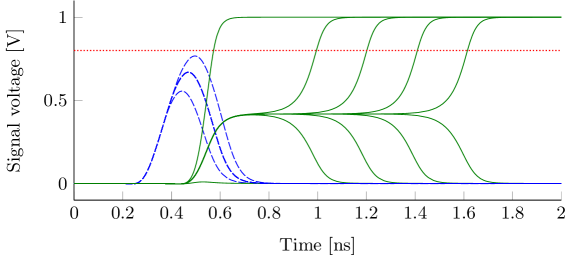
Figure 1: Analog simulation traces of a CMOS SPF, implemented as a storage loop followed by a high-threshold filter. The dashed (blue) curves represent the input signal, the solid (green) ones give the output of the storage loop. The horizontal line at 0.8 marks the filter threshold level.

Figure 2: Input/output signal of a single-history channel, involving the input-to-previous-output delay $T$ and the resulting output-to-input delay $\delta(T)$

A single-history channel, as introduced in [FNS13], is characterized by a delay function $\delta(T)$ that may depend on the difference $T$ between the time of the input transition and that of the previous output transition. Fig. 2 illustrates this relation and the involved delays. Pure delay, inertial delay, and PID channels are all single-history channels with an upper and lower bounded delay function. Interestingly, as shown in [FNS13], binary circuit models based on channels with pure (= constant) delays do not even allow to solve unbounded SPF. On the other hand, bounded single-history channels with non-constant delays, including inertial delay and PID channels, allow to design circuits that solve bounded SPF. Since this contradicts reality, as argued above, none of the existing binary circuit models can faithfully capture glitch propagation.

In this paper, we propose a class of single-history channel models with unbounded delay functions: Like their bounded counterparts, their delay is upper bounded; however, it is not bounded from below. As shown in Section 4, these negative delays are crucial for accurately modeling glitch suppression. We coined the term involution channel for our channels, as we require their negative delay functions to be involutions, i.e., $-\delta(T)$ must form its own inverse (which implies that $\delta(T)$ is strictly increasing and concave). To increase the size of our class of involution channels, we actually allow the delay functions $\delta_{\uparrow}$ and $\delta_{\downarrow}$ for rising and falling transitions to be different, and require both $-\delta_{\downarrow}(-\delta_{\uparrow}(T))=T$ and $-\delta_{\uparrow}(-\delta_{\downarrow}(T))=T$. We will prove that the solvability/unsolvability border of SPF in a binary-valued circuit model based on our involution channels is exactly the same as in reality. It is hence, to the best of our knowledge, the very first candidate for a model that indeed guarantees faithful glitch propagation.

Major contributions and paper organization: (1) In Section 2, we use a simple analog channel model to demonstrate that assuming delay functions which are involutions is not artificial and hence not unrealistic: It reveals that the standard first-order model used e.g. in [RCS90] actually gives a simple instance of general involution channels, which are introduced formally in Section 4. Our binary circuit model, as well as the SPF problem, are formally defined in Section 3. (2) In Section 6, we prove that the simple circuit consisting of a storage loop and a high-threshold filter solves unbounded SPF in the involution channel model. (3) In Section 7, we show that bounded SPF is impossible to solve with involution channels. In a nutshell, our proof inductively constructs an execution that can determine the final output only after some unbounded time. It exploits a surprising continuity property of the output of an involution channel with respect to the presence/absence of glitches at the channel input, which is due to the involution property (unboundedness) of the delay functions.

Together, our results reveal that involution channels indeed allow to solve (bounded) SPF precisely when this is possible in physical circuits, rendering them promising candidates for faithful glitch propagation models.

Related Work. We are not aware of much existing work that relates to the problem studied in our paper: Unger [Ung71] proposed a general technique for modeling asynchronous sequential switching circuits, based on combinational circuit elements interconnected by pure and inertial delay channels. Brzozowski and Ebergen [BE92] formally proved that it is impossible to implement Muller C-Elements and other state-holding components using only zero-time logical gates interconnected by wires without timing restrictions. Bellido-Díaz et al. [BDJCAVH00] proposed the PID model, and justified its appropriateness both analytically and by comparing the model predictions against SPICE simulations. However, as already mentioned, Függer et al. [FNS13] showed that none of the above binary circuit models can faithfully model glitch propagation in physical circuits.

2 The Expressive Power of Involution Channels

Restricting delay functions to satisfy the involution property $-\delta_{\uparrow}(-\delta_{\downarrow}(T))=-\delta_{\downarrow}(-\delta_{\uparrow}(T))=T$ might raise concerns about whether such an assumption makes sense at all in real circuits, and whether/how it fits to existing analog models [NP73:spice, Ho84:thesis, LM84, PR90, DS90]. In this section, we will show that involution channels are indeed well-suited for modeling physical circuits, in the sense that they arise naturally in a (generalized) standard analog model.

More specifically, we will show that, for any given involutions $\delta_{\uparrow}$, $\delta_{\downarrow}$, there is a generalized standard analog channel model consisting of a pure delay component, a slew-rate limiter with generalized switching waveforms, and a comparator, as shown in Fig. 3, which has $\delta_{\uparrow}$, $\delta_{\downarrow}$ as its corresponding delay functions. Note carefully, though, that we do not claim that Fig. 3 is the only analog model that leads to involution delay functions; there may of course be many others as well. Vice versa, the fact that some well-known analog model leads to involutions does not at all make our results incremental: Besides the fact that, to the best of our knowledge, no analog modeling paper [NP73:spice, Ho84:thesis, LM84, PR90, DS90] addressed the properties of corresponding delay functions, it is of course not possible to generalize results obtained for some particular involution to involutions in general.

As a first observation, note that, while allowing separate functions $\delta_{\uparrow}$ for rising and $\delta_{\downarrow}$ for falling transitions, the timing behavior of involution channels is fully determined by either one, as $\delta_{\uparrow}(T)=-\delta_{\downarrow}^{-1}(-T)$ (and similarly for $\delta_{\downarrow}$). To better understand how our delay functions “integrate” the behavior of both transitions, consider the ansatz

$$\begin{split}\delta_{\uparrow}(T)=-f_{\uparrow}^{-1}(f_{\downarrow}(T))\quad\text{ and }\quad\delta_{\downarrow}(T)=-f_{\downarrow}^{-1}(f_{\uparrow}(T)),\end{split}$$ (1)

where $f_{\uparrow}$ resp. $f_{\downarrow}$ are strictly increasing resp. decreasing functions. Note that such functions can be found for any involution $\delta$ function. Intuitively, we would like $f_{\uparrow}$ and $f_{\downarrow}$ to represent the continuous switching waveforms of the output of the generalized slew rate limiter upon the occurrence of a rising respectively falling transition at its input. In the above formula, e.g., at a rising transition, $\delta_{\uparrow}(T)$ returns the time by which $f_{\uparrow}$ has to be shifted so that the output signal remains continuous with respect to the output caused by the previous falling transition. For realistic switching waveforms, we further need $f_{\uparrow}(0)=1-f_{\downarrow}(0)=0$ and $\lim_{t\to\infty}f_{\uparrow}(t)=1-\lim_{t\to\infty}f_{\downarrow}(t)=1$, which requires to augment (1) with some additive terms, resulting in

$$\begin{split}\delta_{\uparrow}(T)=-f_{\uparrow}^{-1}(f_{\downarrow}(T+\delta^{\downarrow}_{\infty}))+\delta^{\uparrow}_{\infty}\text{~{}~{}and~{}~{}}\delta_{\downarrow}(T)=-f_{\downarrow}^{-1}(f_{\uparrow}(T+\delta^{\uparrow}_{\infty}))+\delta^{\downarrow}_{\infty},\end{split}$$ (2)

where $\delta^{\uparrow}_{\infty}$ and $\delta^{\downarrow}_{\infty}$ denote $\lim_{T\to\infty}\delta_{\uparrow}(T)$ and $\lim_{T\to\infty}\delta_{\downarrow}(T)$, respectively.

 

Figure 3: Simple analog channel model.

Fig. 3 shows a block diagram of an idealized analog circuit corresponding to so constructed involution channels, and a sample waveform. The pure delay shifts the binary-valued input $u_{i}$ in time by some $T_{p}$. The slew rate limiter exchanges the step functions of the resulting $u_{d}$ with instances of $f_{\uparrow}$ and $f_{\downarrow}$, shifting them in time such that the output $u_{r}$ is continuous and switches between strictly increasing and decreasing exactly at $u_{d}$ switching times. The comparator generates $u_{o}$ by again discretizing the value of this waveform comparing it to the threshold voltage $V_{th}$, effectively adding $f_{\uparrow}^{-1}(V_{th})$ resp. $f_{\downarrow}^{-1}(V_{th})$ to the instantiation times of $f_{\uparrow}$ resp. $f_{\downarrow}$. The input-output delay of a perfectly idle channel (the last output transition was at time $-\infty$), i.e. $\delta^{\uparrow}_{\infty}$ and $\delta^{\downarrow}_{\infty}$ for rising respectively falling transitions, is the sum of the pure delay and the time the switching waveform needs to reach the threshold voltage $V_{th}$; e.g., for a rising transition, $\delta^{\uparrow}_{\infty}=T_{p}+f_{\uparrow}^{-1}(V_{th})$.

Apart from showing that, for any $\delta$ function, there is a combination of pure delay $T_{p}$, switching waveforms $f_{\uparrow}$ and $f_{\downarrow}$, and threshold $V_{th}$ so that the circuit in Fig. 3 behaves exactly like the corresponding involution channel, (2) can also be used to directly transform the parameters of the model in Fig. 3 to the corresponding $\delta$ function. As a special case, consider a slew rate limiter implemented as a first-order RC low pass filter; the switching waveforms are $f_{\downarrow}(t)=1-f_{\uparrow}(t)=e^{-t/\tau}$ here, with $\tau$ being the RC time constant. Inserting these functions and their inverses into (2) and substituting $\delta^{\uparrow}_{\infty}$ and $\delta^{\downarrow}_{\infty}$ with the corresponding sums of pure delay and comparator delay, we obtain

$$\begin{split}\delta_{\uparrow}(T)&=\tau\ln(1-e^{-(T+T_{p}-\tau\ln(V_{th}))/\tau})+T_{p}-\tau\ln(1-V_{th})\\ \delta_{\downarrow}(T)&=\tau\ln(1-e^{-(T+T_{p}-\tau\ln(1-V_{th}))/\tau})+T_{p}-\tau\ln(V_{th}).\end{split}$$

In the remainder of this paper, these specific (well-known) channels will be called exp-channels.

3 Binary Circuit Model

Since the purpose of our work is to replace analog models like the one in the previous section by a purely digital model, we will now formally define the binary-value continuous-time circuit model used in the remainder of this paper. Except for the involution channels introduced in Section 4, it is essentially the same as the model introduced in [FNS13].

Signals. A falling transition at time $t$ is the pair $(t,0)$, a rising transition at time $t$ is the pair $(t,1)$. A signal is a (finite or infinite) list of alternating transitions such that

1. the initial transition is at time $-\infty$; all other transitions are at times $t\geq 0$,

2. the sequence of transition times is strictly increasing,

3. if there are infinitely many transitions in the list, then the set of transition times is unbounded.

To every signal $s$ corresponds a function $\mathds{R}_{+}\to\{0,1\}$ whose value at time $t$ is that of the most recent transition. We follow the convention that the function already has the new value at the time of a transition, i.e., the function is constant in the half-open interval $[t_{n},t_{n+1})$ if $t_{n}$ and $t_{n+1}$ are two consecutive transition times. A signal is uniquely determined by such a function and its value at $-\infty$.

Circuits. Circuits are obtained by interconnecting a set of input ports and a set of output ports, forming the external interface of a circuit, and a set of combinational gates via channels. We constrain the way components are interconnected in a natural way, by requiring that any gate input, channel input and output port is attached to only one input port, gate output or channel output. Moreover, gates and channels must alternate on every path in the circuit.

Formally, a circuit is described by a directed graph where:

1. Vertices are partitioned into input ports, output ports, channels, and gates.

2. Input ports have no incoming edges and at least one outgoing edge.

3. Output ports have exactly one incoming edge from a gate and no outgoing edges.

4. Channels are nodes that have exactly one incoming and exactly one outgoing edge. Every channel is assigned a channel function, which maps the input to the output. Section 4 specifies the properties of this function for our involution channels.

5. Every gate is assigned a Boolean function $\{0,1\}^{d}\to\{0,1\}$, where $d$ is the number of incoming edges.

6. There is a fixed order on the incoming edges of every gate.

7. Gates and channels alternate on every path in a circuit.

Executions. An execution of circuit $C$ is an assignment of signals to vertices that respects the channel functions and Boolean gate functions.

Formally, an execution of circuit $C$ is a collection of signals $s_{v}$ for all vertices $v$ of $C$ such that the following properties hold:

1. If $i$ is an input port, then there are no restrictions on $s_{i}$.

2. If $o$ is an output port, then $s_{o}=s_{v}$, where $v$ is the unique gate $v$ associated with $o$.

3. If $c$ is a channel, then $s_{c}=f_{c}(s_{v})$, where $v$ is the unique incoming neighbor of $c$ and $f_{c}$ the channel function.

4. If $b$ is a gate with $d$ incoming neighbors $v_{1},\dots,v_{d}$, ordered according to the fixed order of condition (C6), and gate function $f_{b}$, then for all times $t$,

   $$s_{b}(t)=f_{b}\big{(}s_{v_{1}}(t),s_{v_{2}}(t),\dots,s_{v_{d}}(t)\big{)}\enspace.$$

Short-Pulse Filtration. A pulse of length $\Delta$ at time $T$ has initial value $0$, one rising transition at time $T$, and one falling transition at time $T+\Delta$. A signal contains a pulse of length $\Delta$ at time $T$ if it contains a rising transition at time $T$, a falling transition at time $T+\Delta$ and no transition in between.

A circuit solves Short-Pulse Filtration (SPF) if it fulfills the following conditions. Note that we allow the circuit to behave arbitrarily if the input signal is not a (single) pulse.

1. The circuit has exactly one input port and exactly one output port. (Well-formedness)

2. If the input signal is the zero signal, then so is the output signal. (No generation)

3. There exist an input pulse such that the output signal is not the zero signal. (Nontriviality)

4. There exists an $\varepsilon>0$ such that for every input pulse the output signal never contains a pulse of length less than $\varepsilon$. (No short pulses)

A circuit solves bounded SPF if additionally the following condition holds:

1. There exists a $K>0$ such that for every input pulse the last output transition is before time $T+K$ if $T$ is the time of the last input transition. (Bounded stabilization time)

4 Involution Channels

Intuitively, a channel propagates each transition at time $t$ of the input signal to a transition at the output happening after some output-to-input delay $\delta(T)$, which depends on the input-to-previous-output delay $T$. Note that $T$ can be negative if two input transitions are close together, as is the case in Fig. 4.

Figure 4: Input transition with negative input-to-last-output delay $T$

Formally, an involution channel is characterized by an initial value $I\in\{0,1\}$ and two strictly increasing concave delay functions $\delta_{\uparrow}:(-\delta^{\downarrow}_{\infty},\infty)\to(-\infty,\delta^{\uparrow}_{\infty})$ and $\delta_{\downarrow}:(-\delta^{\uparrow}_{\infty},\infty)\to(-\infty,\delta^{\downarrow}_{\infty})$ such that both $\delta^{\uparrow}_{\infty}=\lim_{T\to\infty}\delta_{\uparrow}(T)$ and $\delta^{\downarrow}_{\infty}=\lim_{T\to\infty}\delta_{\downarrow}(T)$ are finite and

$$-\delta_{\uparrow}\big{(}-\delta_{\downarrow}(T)\big{)}=T\text{ and }-\delta_{\downarrow}\big{(}-\delta_{\uparrow}(T)\big{)}=T$$ (3)

for all applicable $T$. All such functions are necessarily continuous and strictly increasing. For simplicity, we will also assume them to be differentiable; $\delta$ being concave thus implies that its derivative $\delta^{\prime}$ is monotonically decreasing. If multiple channels in a circuit share a common input signal, as depicted in Fig. 5, we require that they all have the same initial value $I$. This is without loss of generality, as one can always replicate the input signal.

Figure 5: A circuit (graph) with vertex $v$ (being an input or a gate), gates $w$, $z$, and channels $c_{1}$ and $c_{2}$ (on the left) and the physical equivalent (on the right). Both channels must have the same initial value $I$; $b$ and $b^{\prime}$ are the Boolean functions assigned to gates $w$ and $z$, respectively.

The behavior of involution channels is defined as follows:

Initialization: If the channel’s initial value $I$ is different from the initial value $X$ of the channel input signal $s$ and $s$ has no transition at time $0$, add the transition $(0,X)$ at time $0$ to $s$ (“reset”).

Output transition generation algorithm: Let $t_{1},t_{2},\dots$ be the times of the transitions of $s$, and set $t_{0}=-\infty$ and $\delta_{0}=0$.

• Iteration: Determine the tentative list of pending output transitions: Recursively determine the output-to-input delay $\delta_{n}$ for the input transition at time $t_{n}$ by setting $\delta_{n}=\delta_{\uparrow}(t_{n}-t_{n-1}-\delta_{n-1})$ if $t_{n}$ is a rising transition and $\delta_{n}=\delta_{\downarrow}(t_{n}-t_{n-1}-\delta_{n-1})$ if it is falling. The $n$th and $m$th pending output transitions cancel if $n<m$ but $t_{n}+\delta_{n}\geq t_{m}+\delta_{m}$. In this case, we mark both as canceled.

• Return: The channel output signal $c(s)$ has initial value $I$ and contains every pending transition at time $t_{n}+\delta_{n}$ that has not been marked as canceled.

Definition 1.

An involution channel is strictly causal if $\delta_{\uparrow}(0)>0$, which is equivalent to the condition $\delta_{\downarrow}(0)>0$ due to (3).

Lemma 2.

An exp-channel is strictly causal if and only if $T_{p}>0$.

The next lemma identifies an important parameter $\delta_{\min}$ of a strictly causal involution channel, which gives its minimal pure delay.

Lemma 3.

A strictly causal involution channel has a unique $\delta_{\min}$ defined by $\delta_{\uparrow}(-\delta_{\min})=\delta_{\min}=\delta_{\downarrow}(-\delta_{\min})$, which is positive. For exp-channels, $\delta_{\min}=T_{p}$.

For the derivative, we have $\delta_{\uparrow}^{\prime}(-\delta_{\downarrow}(T))=1/\delta_{\downarrow}^{\prime}(T)$ and hence $\delta_{\uparrow}^{\prime}(-\delta_{\min})=1/\delta_{\downarrow}^{\prime}(-\delta_{\min})$.

Proof.

Set $f(T)=-T+\delta_{\uparrow}(-T)$. This function is continuous and strictly decreasing, since $\delta_{\uparrow}$ is continuous and strictly increasing. Because $f(0)=\delta_{\uparrow}(0)$ is positive and the limit of $f(T)$ as $T\to\delta^{\downarrow}_{\infty}$ is $-\infty$, there exists a unique $\delta_{\min}$ between $0$ and $\delta^{\downarrow}_{\infty}$ for which $f(\delta_{\min})=0$. Hence, $\delta_{\uparrow}(-\delta_{\min})=\delta_{\min}$. The second equality follows from $\delta_{\min}=\delta_{\downarrow}(-\delta_{\uparrow}(-\delta_{\min}))=\delta_{\downarrow}(-\delta_{\min})$ according to (3).

The second part of the lemma follows by differentiating Equation (3). ∎

We next show that $\delta_{\min}$ indeed deserves its name: A particular consequence of the following lemma is that the channel delay for any non-canceled transition is at least $\delta_{\min}$.

Lemma 4.

The $n$th and $(n+1)$th pending output transitions cancel if and only if $t_{n+1}\leq t_{n}+\delta_{n}-\delta_{\min}$.

Proof.

Let $\delta$ be either $\delta_{\uparrow}$ or $\delta_{\downarrow}$, depending on whether $t_{n+1}$ is a rising or falling transition. By definition, the two transitions cancel if and only if

$$\delta_{n+1}=\delta(t_{n+1}-t_{n}-\delta_{n})\leq-(t_{n+1}-t_{n}-\delta_{n})\enspace.$$ (4)

Set $T=t_{n+1}-t_{n}-\delta_{n}$. By Lemma 3, equality holds in (4) if and only if $T=-\delta_{\min}$. Because the left-hand side of (4) is increasing in $T$ and the right-hand side is strictly decreasing in $T$, (4) is equivalent to $T\leq-\delta_{\min}$, which in turn is equivalent to $t_{n+1}\leq t_{n}+\delta_{n}-\delta_{\min}$. ∎

In the rest of the paper, we assume all channels to be strictly causal involution channels.

5 Constructing Executions of Circuits

The definition of an execution of a circuit as given in Section 3 is “existential”, in the sense that it only allows to check for a given collection of signals whether it is an execution or not. And indeed, in general, circuits may have no execution or may have several different executions. By contrast, in case of circuits involving strictly causal involution channels only, executions are unique and can be constructed iteratively: We give a deterministic construction algorithm below.

Given a circuit $C$ with strictly causal involution channels, let $(s_{i})_{i\in\mathcal{I}}$ be any collection of signals for all the input ports $\mathcal{I}$. Since all output ports are driven by gates we can identify the output port with the output of its driving gate. The channel with predecessor $x$ (an input port or a gate output) and successor $y$ (a gate input) is denoted by the tuple $(x,y)$. The algorithm iteratively generates the list of transitions of $s_{\sigma}$ of (the output of) every vertex $\sigma$ in the circuit, and hence the corresponding function $s_{\sigma}(t)$. In the course of the execution of this algorithm, a subset of the generated transitions will be marked fixed: Non-fixed transitions could still be canceled by other transitions later on, fixed transitions will actually occur in the constructed execution.

The detailed algorithm is as follows:

Initialization: For all channels $(v,w)$ in $C$, $s_{(v,w)}=((-\infty,I))$ initially, with $I$ being the initial value of channel $(v,w)$. According to the implicit reset of our channels introduced in Section 4, the transition $(0,X)$ is also added to $s_{(v,w)}$ if the initial transition $(-\infty,X)$ of $s_{v}$ satisfies $X\neq I$. For a gate $v$, $s_{v}=((-\infty,X))$ initially, where $X$ is the value of the Boolean function corresponding to $v$ applied to the values of the initial transitions in $s_{\sigma}$ for all of $v$’s predecessors $\sigma$. The zero-input gates $0$ and $1$ used for generating constant-0 and constant-1 signals have $s_{0}=((-\infty,0))$ and $s_{1}=((-\infty,1))$, respectively. Initially, all transitions at $-\infty$ are fixed and all others are not.

Iteration: If there is no non-fixed transition left, terminate with the execution made up by all fixed transitions. Otherwise, let $t\geq 0$ be the smallest time of a non-fixed transition.

1. Mark all transitions at $t$ fixed.

2. For each newly fixed transition from step (i), occurring in $s_{\sigma}$ where $\sigma$ is a predecessor of a gate $v$: If signal $s_{v}$’s current value $s_{v}(t)=X$ differs from the value of $v$’s Boolean function applied to the values $s_{\sigma^{\prime}}(t)$ for all of $v$’s predecessors $\sigma^{\prime}$ (which also include $\sigma$), add the transition $(t,1-X)$ to $s_{v}$ and mark it fixed.

3. For each newly fixed transition $(t,x)\in s_{v}$ from steps (i) or (ii), occurring in $s_{v}$ of a gate output or an input port: For each successor channel $(v,w)$ of $v$, apply the iteration step of $(v,w)$’s transition generation algorithm with input signal $s_{v}$, output signal $s_{(v,w)}$, and current input transition $(t,X)$. If this leads to a cancellation in $s_{(v,w)}$, remove both canceling and canceled transition from the list. Lemma 7 will show that no fixed transition will ever be removed this way.

We will now show that this algorithm indeed constructs an execution of $C$. Let $t_{\ell}$ be the smallest finite time of non-fixed transitions at the beginning of iteration $\ell\geq 1$ of the algorithm, and denote by $\delta^{C}_{\min}>0$ the minimal $\delta_{\min}$ of all channels in circuit $C$.

Lemma 5.

For all iterations $\ell\geq 1$, (a) no transition $(t,X)$ with $t\neq t_{\ell}$ is newly marked fixed in the iteration, (b) a transition $(t,X)$ added during and not removed by the end of iteration $\ell$ either has time $t=t_{\ell}$ or $t>t_{\ell}+\delta_{\min}^{C}>t_{\ell}$, and (c) every transition at time $t_{\ell}$ is fixed at the end of the iteration.

Proof.

Statement (a) is implied by the fact that transitions are only marked fixed in step (i) and (ii), which act on transitions at time $t_{\ell}$ only.

For (b), assume by contradiction that a transition $(t,X)$ with $t\leq t_{\ell}+\delta_{\min}^{C}$ but different from $t_{\ell}$ was added in iteration $\ell$ and still exists at the end of iteration $\ell$. Such a transition can only be added via step (iii). For the respective channel algorithm with delay function $\delta$, $\delta(t_{\ell}-t^{\prime})\leq\delta_{\min}^{C}$ must have held, where $t^{\prime}$ is the time of the channel’s last output transition. From Lemma 3, we deduce that this implies $t_{\ell}\leq t^{\prime}-\delta_{\min}$ for the particular channel’s minimal delay $\delta_{\min}$, since $\delta_{\min}^{C}\leq\delta_{\min}$. By Lemma 4, this leads to a cancellation and hence removal of $(t,X)$, which provides the required contradiction.

For (c), assume by contradiction that, at the end of iteration $\ell$, there exists a non-fixed transition $(t_{\ell},X)$. Since step (i) marks all transitions at time $t_{\ell}$ fixed and (ii) adds only fixed transitions at time $t_{\ell}$, the non-fixed transition must have been newly added in step (iii). However, from (b), we know that this requires $t>t_{\ell}+\delta_{\min}^{C}>t_{\ell}$, a contradiction. ∎

From an inductive application of Lemma 5, we obtain that the sequence of iteration start times $(t_{\ell})_{\ell\geq 1}$ is strictly increasing without bound:

Lemma 6.

For all iterations $\ell>1$, $t_{\ell}-t_{\ell-1}>0$. If $t_{\ell}$ does not involve an input transition, then $t_{\ell}-t_{\ell-1}>\delta_{\min}^{C}$.

Proof.

By Lemma 5 (b), $t_{\ell+1}$ is larger than $t_{\ell}+\delta_{\min}^{C}$, provided no input transition occurs earlier. As we do not allow Zeno behavior of input signals, $t_{\ell}-t_{\ell-1}>0$ is guaranteed also in the latter case. ∎

The following lemma proves that the generated event lists are well-defined, in the sense that no later iteration can remove events that may have generated causally dependent other events already.

Lemma 7.

No fixed transition is canceled in any iteration.

Proof.

Assume by contradiction that some iteration $\ell\geq 2$ is the first in which a fixed transition is canceled; obviously, this can only happen in step (iii). Thus, there exists a transition at time $t_{\ell}$ that generated a new transition at some time $t$ that results in the cancellation of a fixed transition at time $t^{\prime}$, i.e., $t\leq t^{\prime}$. Lemma 4 implies that $t_{\ell}-t^{\prime}\leq-\delta_{\min}<0$ in this case. By Lemma 5.(a)–(c), however, $t\leq t^{\prime}\leq t_{\ell}$ and thus $t_{\ell}-t^{\prime}\geq 0$, which provides the required contradiction. ∎

We are now ready for the main result of this section, which asserts the existence of a unique execution of our circuit $C$:

Theorem 8.

The execution construction algorithm either terminates or, for all times $T\geq 0$, there exists an iteration $\ell$ such that $t_{\ell}\geq T$. At the end of iteration $\ell\geq 1$, the collection of signals $s_{\sigma}$, restricted to time $[-\infty,t_{\ell}]$, is the unique execution of circuit $C$ restricted to time $[-\infty,t_{\ell}]$. If the algorithm terminates at the beginning of iteration $\ell$, then this collection of signals is the unique execution of circuit $C$.

Proof.

From Lemma 6, we deduce that for all times $t\geq 0$, there is an iteration $\ell\geq 1$ such that $t_{\ell}>t$ or the algorithm terminates. From Lemma 7, we further know that in both cases the algorithm does not add transitions with times less or equal to $t$. Uniqueness of the execution follows from the fact that the construction algorithm is deterministic. ∎

6 Possibility of Unbounded Short-Pulse Filtration

In this section, we show that unbounded SPF is solvable in our circuit model with strictly causal involution channels. We do this by verifying that the circuit shown in Fig. 6 indeed solves SPF. The circuit was inspired by the physical solution of Fig. 1, and consists of a fed back OR-gate forming the storage loop and a subsequent high-threshold filter (implemented by a channel). In order not to obfuscate the essentials (and to stick to the page limit), we restrict our attention to certain classes of involution channels. More specifically, in our proof, the channel in the feed-back loop must be strictly causal and symmetric, i.e., $\delta_{\uparrow}=\delta_{\downarrow}=\delta$. When using an exp-channel, for example, this implies a threshold $V_{th}=0.5$. The channel implementing the high-threshold filter is assumed to be an exp-channel because we have to adjust its parameters appropriately.

Figure 6: A circuit solving unbounded SPF, consisting of an OR-gate fed back by channel $c$, and a high-threshold filter HT.

We consider a pulse of length $\Delta$ at time $0$ at the input and reason about the behavior of the feed-back loop. Then, we show that this behavior can be translated to a legitimate SPF output by using a high-threshold filter. We start by identifying two extremal cases: If $\Delta$ is too small, then the pulse is filtered by the channel in the feed-back loop. If it is too big, the pulse is captured by the storage loop, leading to a stable output 1.

Lemma 9.

If the input pulse’s length $\Delta$ satisfies $\Delta\geq\delta_{\infty}$, then the output of the OR has a unique rising transition at time $\delta_{\infty}$.

Proof.

Assigning the channel output $s_{c}$ a single rising transition at time $\delta_{\infty}$ is part of a consistent execution, in which the OR’s output has a single rising transition at time $0$. The lemma now follows from uniqueness of executions. ∎

Lemma 10.

If the input pulse’s length $\Delta$ satisfies $\Delta\leq\delta_{\infty}-\delta_{\min}$, then the OR output contains only the input pulse.

Proof.

The input signal contains only two transitions: One at time $t_{1}=0$ and one at time $t_{2}=\Delta\leq\delta_{\infty}-\delta_{\min}$. Since $\delta_{1}=\delta_{\infty}$ and hence $t_{2}=t_{1}+\Delta\leq t_{1}+\delta_{1}-\delta_{\min}$, the two pending transitions of $c$’s output cancel by Lemma 4, and no further transitions are generated afterwards. ∎

Now suppose that the input pulse length satisfies $\delta_{\infty}-\delta_{\min}<\Delta_{0}<\delta_{\infty}$. For these pulse lengths $\Delta_{0}$, the OR output signal will contain a series of pulses of lengths $\Delta_{0},\Delta_{1},\Delta_{2},\dots$ For all but one $\Delta_{0}$, this series will turn out to be either decreasing or increasing and finite, causing the output signal to be eventually $0$ or eventually $1$. To compute these pulse lengths, we define the auxiliary function

$$f(\Delta)=\delta\big{(}\Delta-\delta(-\Delta)\big{)}+\Delta-\delta(-\Delta)\enspace,$$ (5)

which gives $\Delta_{n}=f(\Delta_{n-1})$ for all $n\geq 2$. To see this, note that $\Delta_{n-1}$ at the channel input is also present at the channel output, so the rising resp. falling transition is delayed by $\delta(-\Delta_{n-1})$ resp. $\delta(\Delta_{n-1}-\delta(-\Delta_{n-1}))$. The first generated pulse starts from a zero channel input and thus

$$\Delta_{1}=\Delta_{0}-\delta_{\infty}+\delta(\Delta_{0}-\delta_{\infty}).$$ (6)

The procedure stops if either $f(\Delta_{n})\leq 0$ (pulse canceled; the output is constant $0$ thereafter), or if

$$f(\Delta_{n})\geq\delta(0)>0$$ (7)

(pulse captured; the output is constant $1$ thereafter).

The only case in which the procedure does not stop is if $f(\Delta_{1})=\Delta_{1}$. There is a unique $\Delta_{1}>0$ with this property, denoted $\tilde{\Delta}_{1}$. By (5), it is also characterized by the relation $\delta(-\tilde{\Delta}_{1})=2\tilde{\Delta}_{1}$. Since $\delta(-\delta(0))=0$ by the involution property, we must have $\tilde{\Delta}_{1}<\delta(0)$. Since $\Delta_{1}\to\delta(0)$ as $\Delta_{0}\to\delta_{\infty}$ and $\Delta_{1}\to 0$ as $\Delta_{0}\to\delta_{\infty}-\delta_{\min}$, there exists a unique $\Delta_{0}$ such that $\Delta_{1}=\tilde{\Delta}_{1}$. Denote it by $\tilde{\Delta}_{0}$.

The following lemma shows that the procedure indeed stops if and only if $\Delta_{1}\neq\tilde{\Delta}_{1}$, and can be used to bound the number of steps until it stops.

Lemma 11.

$\lvert f(\Delta_{1})-\tilde{\Delta}_{1}\rvert\geq(1+\delta^{\prime}(0))\cdot\lvert\Delta_{1}-\tilde{\Delta}_{1}\rvert$ if $\Delta_{1}>0$.

Proof.

We have

$$\begin{split}f^{\prime}(\Delta_{1})=&\big{(}1+\delta^{\prime}(-\Delta_{1})\big{)}\cdot\delta^{\prime}\big{(}\Delta_{1}-\delta(-\Delta_{1})\big{)}\\ &+1+\delta^{\prime}(-\Delta_{1})\geq 1+\delta^{\prime}(0)\end{split}$$ (8)

because $\delta^{\prime}(-\Delta_{1})\geq\delta^{\prime}(0)$ and $\delta^{\prime}(T)>0$ for all $T$ as $\delta$ is concave and increasing. The mean value theorem of calculus now implies the lemma. ∎

Theorem 12.

The fed-back OR gate with a strictly causal symmetric involution channel has the following output when the input pulse has length $\Delta_{0}$:

• If $\Delta_{0}>\tilde{\Delta}_{0}$, then the output is eventually constant $1$.

• If $\Delta_{0}<\tilde{\Delta}_{0}$, then the output is eventually constant $0$.

• If $\Delta_{0}=\tilde{\Delta}_{0}$, then the output is a periodic pulse train with duty cycle 50%.

Furthermore, the stabilization time in the first two cases is in the order of $\log(1/\lvert\Delta_{0}-\tilde{\Delta}_{0}\rvert)$.

Proof.

If $\Delta_{0}\geq\delta_{\infty}$ or $\Delta_{0}\leq\delta_{\infty}-\delta_{\min}$, then Lemmas 9 and 10 show the theorem.

So let $\Delta_{0}\in(\delta_{\infty}-\delta_{\min},\delta_{\infty})$. By Lemma 11, the number of generated pulses until the procedure stops is in the order of $\log 1/\lvert\Delta_{1}-\tilde{\Delta}_{1}\rvert$. Setting $g(\Delta_{0})=\Delta_{0}-\delta_{\infty}+\delta(\Delta_{0}-\delta_{\infty})$ such that $\Delta_{1}=g(\Delta_{0})$, cp. (6), and applying the mean value theorem of calculus to this function, we see analogously as in the proof of Lemma 11 that

$$\lvert\Delta_{1}-\tilde{\Delta}_{1}\rvert\geq\big{(}1+\delta^{\prime}(0)\big{)}\cdot\lvert\Delta_{0}-\tilde{\Delta}_{0}\rvert\enspace.$$

Hence the number of generated pulses is in the order of $\log 1/\lvert\Delta_{0}-\tilde{\Delta}_{0}\rvert$. Since both the length $\Delta_{n}$ of the occurring pulses and, by symmetry, the time between them is at most $\delta(0)$ since it would be captured otherwise, cp. (7), we have the same asymptotic bound on the stabilization time. ∎

We now turn to the analysis of the high-threshold filter.

Lemma 13.

Let $c$ be an exp-channel $c$ with threshold $V_{th}$. Then there exists some $\Delta>0$ such that every periodic pulse train with pulse lengths at most $\Delta$ and duty cycle (ratio of 1-to-0) at most $V_{th}$ is mapped to the zero signal by $c$.

Proof.

Let $t_{1},t_{2},\dots$ be the times of transitions in the input pulse train with duty cycle $\gamma\leq V_{th}$, i.e., $t_{1}=0$, $t_{2n+2}=t_{2n+1}+\Delta$, and $t_{2n+1}=t_{2n}+\Delta/\gamma$. We assume that $\Delta$ is smaller than both $-\tau\log(1-V_{th})$ and a to-be-determined $\Delta_{0}$, and show inductively that all pulses get canceled:

If $\Delta\leq-\tau\log(1-V_{th})$, then $\delta_{1}=\delta_{\uparrow}(\infty)=T_{p}-\tau\log(1-V_{th})>T_{p}$ and $\delta_{2}=\delta_{\downarrow}(\Delta-\delta_{1})\leq T_{p}$, so the first pulse is canceled. For the induction step, we assume $\delta_{2n}\leq T_{p}$ and find

$$\begin{split}\delta_{2n+1}&=\delta_{\uparrow}(\Delta/\gamma-\delta_{2n})\geq\delta_{\uparrow}(\Delta/V_{th}-T_{p})\\ &=T_{p}-\tau\log(1-V_{th})+\tau\log(1-V_{th}e^{-\Delta/V_{th}\tau})\end{split}$$

Hence, $t_{2n+1}$ and $t_{2n+2}=t_{2n+1}+\Delta$ cancel if

$$\begin{split}\Delta&\leq\delta_{2n+1}-T_{p}\\ &=-\tau\log(1-V_{th})+\tau\log(1-V_{th}e^{-\Delta/V_{th}\tau})\enspace,\end{split}$$

which is equivalent to

$$\begin{split}h(\Delta)=V_{th}e^{-\Delta/V_{th}\tau}+(1-V_{th})e^{\Delta/\tau}\leq 1\enspace.\end{split}$$

The latter satisfies $h(0)=1$ and

$$\begin{split}h^{\prime}(\Delta)=-\frac{1}{\tau}e^{-\Delta/V_{th}\tau}+\frac{1-V_{th}}{\tau}e^{\Delta/\tau}\enspace,\end{split}$$

in particular $h^{\prime}(0)=-V_{th}/\tau<0$. There hence exists some $\Delta_{0}>0$ such that $h(\Delta)\leq 1$ for all $0\leq\Delta\leq\Delta_{0}$. Thus, $t_{2n+1}$ and $t_{2n+2}$ cancel, and

$$\begin{split}\delta_{2n+2}&=\delta(\Delta-\delta_{2n+1})\leq\delta(-T_{p})=T_{p}\end{split}$$

because $h(\Delta)\leq 1$, which completes the induction step. ∎

By letting $\tau$ grow, one can even achieve the following result.

Lemma 14.

Let $\hat{\Delta}>0$ and $0<\gamma<1$. Then there exists an exp-channel with threshold $V_{th}=\gamma$ such that every periodic pulse train with pulse lengths at most $\hat{\Delta}$ and duty cycle at most $\gamma$ is mapped to the zero signal by $c$.

Proof.

We use the notation of the proof of Lemma 13. The unique root of $h^{\prime}(\Delta)$ is equal to

$$\Delta_{\tau}=-\frac{\tau\log(1-V_{th})}{1+1/V_{th}}\enspace,$$

which goes to infinity as $\tau\to\infty$. We can choose $\Delta_{0}=\Delta_{\tau}$ because $h^{\prime}(\Delta)\leq 0$ for all $0\leq\Delta\leq\Delta_{\tau}$. Because also $-\tau\log(1-V_{th})$ goes to infinity as $\tau\to\infty$, we can find, for any given $\Delta$, some $\tau>0$ such that both $\Delta\leq-\tau\log(1-V_{th})$ and $\Delta\leq\Delta_{\tau}$. But for these $\Delta$, all input pulse trains with pulse lengths $\Delta$ and duty cycle at most $V_{th}=\gamma$ get mapped to the zero signal. ∎

In particular, by choosing $\gamma=0.6$ and $\hat{\Delta}$ large enough such that the output of the feed-back loop is already constant $1$ at time $T+\hat{\Delta}$ if the duty cycle in the loop passes $0.6$ at time $T$, the critical pulse duration $\tilde{\Delta}_{0}$ is mapped to a zero-output. It hence follows:

Theorem 15.

There is a circuit that solves unbounded SPF.

7 Impossibility of Bounded Short-Pulse Filtration

7.1 Continuity of Channels

In this subsection, we prove that strictly causal channels are continuous in a certain sense that we will define precisely. For ease of exposition and for space reasons, we give the proof only in the case of symmetric channels, i.e., for the case that $\delta_{\uparrow}=\delta_{\downarrow}=\delta$.

We begin by noting that channels are monotone. To compare certain signals, we write $s_{1}\leq s_{2}$ if $s_{2}$ is $1$ whenever $s_{1}$ is.

Lemma 16.

Let $s_{1}$ and $s_{2}$ be signals such that $s_{1}\leq s_{2}$ and let $c$ be a channel. Then, $c(s_{1})\leq c(s_{2})$.

We next define a distance for signals, for which channels will turn out to be continuous.

Definition 17.

For a signal $s$ and a time $T$, denote by $\mu_{T}(s)$ the total duration in $[0,T]$ where $s$ is $1$. In more symbolic terms, $\mu_{T}(s)$ is the measure of the set $\{t\in[0,T]\mid s(t)=1\}$.

For any two signals $s_{1}$ and $s_{2}$ and every $T$, we define their distance up to time $T$ by setting $\lVert s_{1}-s_{2}\rVert_{T}=\mu_{T}(\lvert s_{1}-s_{2}\rvert)$.

Intuitively, an involution channel is continuous under this measure for two reasons: (i) Due to the continuity of $\delta$, a small change in the time at which an input transition occurs, results in a small change in the time at which the corresponding output transition occurs. This, again, only results in a small change of the input-to-previous-output time for the next input transition, and so on. The technical difficulty is to show that this effect does not result in discontinuities even for an unbounded number of input transitions. (ii) Due to the involution property of $\delta$, one can show that $\delta$ is not only continuous in changing the length of input pulses, but also in removing them: An input pulse whose length is arbitrary small results in a value of $\delta$ for the next input transition that is arbitrarily close to the transition’s $\delta$ value in the case the short pulse was not present at all. Again, the major difficulty lies in showing that this also holds for infinite pulse trains.

Note carefully that it is primarily the continuity property (ii) that distinguishes our involution channels from the “unfaithful” single-history channels analyzed in [FNS13], which allow bounded SPF to be solved.

We start our detailed proof with Lemma 18, which provides an optimal choice for appending a pulse at the end of a signal in order to maximize $\mu_{T}$. We will use it later when bounding the maximum impact of an infinitesimally small pulse.

We use the shorthand notation $(x)_{+}$ for $\max(x,0)$.

Lemma 18.

Let $s$ be a signal that is eventually constant $0$ and let $c$ be a channel. Denote by $t_{n}$ the time of the last (falling) transition in $s$ and by $\delta_{n}$ its delay in the channel algorithm for $c$. Then, the maximal $\mu_{T}(c(s^{\prime}))$ among all $s^{\prime}$ obtained from $s$ by appending one pulse of length $\Delta$ after time $t_{n}$ is attained by the addition of the pulse at time $t_{n}+(\delta_{n}-\delta_{\min})_{+}$ (which results in a cancellation, i.e., a right-shift, of the last transition).

Proof.

We first show the lemma for $T=\infty$ and then extend the result to finite $T$. Let $s^{\prime}_{\gamma}$ be the addition of the pulse of length $\Delta$ to $s$ at time $t_{n}+\gamma$.

For all $0\leq\gamma\leq\delta_{n}-\delta_{\min}$, set

$$f(\gamma)=\gamma+\delta(\Delta-\delta(\gamma-\delta_{n}))\enspace.$$

In the class of all $s^{\prime}_{\gamma}$ with $0\leq\gamma\leq\delta_{n}-\delta_{\min}$ (which can be empty), the maximum of $\mu_{T}(c(s^{\prime}_{\gamma}))$ is attained at the maximum of $f$. This is because the transition at time $t_{n}+\gamma$ cancels that at time $t_{n}$ in this case. The derivative of $f$ is equal to

$$f^{\prime}(\gamma)=1-\delta^{\prime}(\Delta-\delta(\gamma-\delta_{n}))\cdot\delta^{\prime}(\gamma-\delta_{n})\enspace.$$

The condition $f^{\prime}(\gamma)=0$ is equivalent to $\delta^{\prime}(\Delta-\delta(\gamma-\delta_{n}))=1/\delta^{\prime}(\gamma-\delta_{n})$, which is in turn equivalent to $\delta(\Delta-\delta(\gamma-\delta_{n}))=-(\gamma-\delta_{n})$, i.e., $\Delta=0$, as $\delta^{\prime}(t)=1/\delta^{\prime}(-\delta(t))$ by Lemma 3. Hence, $f^{\prime}(\gamma)$ is never zero. Since $f^{\prime}(\gamma)\to 1$ as $\gamma\to\infty$, as the concave $\delta$ satisfies $\lim_{t\to\infty}\delta^{\prime}(t)=0$, the derivative of $f$ is always positive, hence $f$ is increasing. This shows that $\gamma=\delta_{n}-\delta_{\min}$ is a strictly better choice than any other $\gamma$ in this class.

For the class of $s^{\prime}_{\gamma}$ with $\gamma\geq(\delta_{n}-\delta_{\min})_{+}>0$, we define the function

$$g(\gamma)=\Delta+\delta(\Delta-\delta(\gamma-\delta_{n}))-\delta(\gamma-\delta_{n})\enspace.$$

Since the transitions at $t_{n}$ and $t_{n}+\gamma$ do not cancel in this class, the maximum of $\mu_{\infty}(c(s^{\prime}_{\gamma}))$ is attained at the maximum of $g$. But it easy to see, using the monotonicity of $\delta$, that $g$ is decreasing. The maximum of $g$ is hence attained at $\gamma=(\delta_{n}-\delta_{\min})_{+}$.

Consequently, the choice $\gamma=\gamma_{0}=(\delta_{n}-\delta_{\min})_{+}$ maximizes $\mu_{\infty}(c(s^{\prime}_{\gamma}))$ in any case. By Lemma 4, this choice results in a cancellation of the last (falling) transition in $s$, hence a right-shift of the latter in $s^{\prime}$. This concludes our proof for $T=\infty$.

Let now $T$ be finite. Denote by $T_{0}$ the time of the last, falling, output transition in $c(s_{\gamma_{0}}^{\prime})$. In this case, transitions of $c(s)$ and $c(s_{\gamma_{0}}^{\prime})$ are the same except the last, falling, transition which is delayed from $t_{n}+\delta_{n}$ to $T_{0}$. We distinguish the two cases (a) $T\leq T_{0}$ and (b) $T>T_{0}$. In case (a), the last transition of $c(s)$ is delayed beyond $T$ in $c(s_{\gamma_{0}}^{\prime})$. Because all other transitions remain unchanged in all $c(s_{\gamma}^{\prime})$, the measure $\mu_{T}(c(s_{\gamma_{0}}^{\prime}))$ is maximal among all $\mu_{T}(c(s_{\gamma}^{\prime}))$ if $T\leq T_{0}$. In case (b), we have $\mu_{T}(c(s_{\gamma_{0}}^{\prime}))=\mu_{\infty}(c(s_{\gamma_{0}}^{\prime}))$. But because $\mu_{T}\leq\mu_{\infty}$ and $\mu_{\infty}(c(s_{\gamma_{0}}^{\prime}))$ is maximal among all $\mu_{\infty}(c(s_{\gamma}^{\prime}))$, so is $\mu_{T}(c(s_{\gamma_{0}}^{\prime}))$ among all $\mu_{T}(c(s_{\gamma}^{\prime}))$. ∎

We next effectively bound the maximum impact on $\mu_{T}$ that a set of pulses of small combined length can have.

Lemma 19.

Let $s$ be a signal that is eventually constant $0$ and let $c$ be a channel. Then there exists a constant $d$ such that the maximal $\mu_{T}(c(s^{\prime}))$ among all $s^{\prime}$ obtained from $s$ by adding pulses of combined length $\varepsilon$ after the last transition of $s$ is at most $\mu_{T}(c(s))+d\cdot\varepsilon$.

Proof.

It suffices to show the lemma for $T=\infty$. Let $\varepsilon=\sum_{k=1}^{\infty}\varepsilon_{k}$. We add, one after the other, pulses of length $\varepsilon_{k}$ after the last transition. We show that the maximum gain after adding $K$ pulses is at most $\sum_{k=1}^{K}\varepsilon_{k}$.

Denote by $t_{n}$ the last transition in $s$ and by $\delta_{n}$ its delay. By Lemma 18, it is optimal to add the first pulse (of length $\varepsilon_{1}$) at time $t_{n}+(\delta_{n}-\delta_{\min})_{+}$; call the resulting signal $s_{1}^{\prime}$.

We first assume $\delta_{n}-\delta_{\min}\geq 0$. Here, the two new transitions in $s_{1}^{\prime}$ are $t_{n+1}=t_{n}+\delta_{n}-\delta_{\min}$ and $t_{n+2}=t_{n}+\delta_{n}-\delta_{\min}+\varepsilon_{1}$. Their corresponding delays are $\delta_{n+1}=\delta_{\min}$ and $\delta_{n+2}=\delta(\varepsilon_{1}-\delta_{\min})$. By the mean value theorem of calculus and Lemma 3, the duration of the resulting pulse is

$$\begin{split}\delta_{n+2}-\delta_{n+1}=\delta(\varepsilon_{1}-\delta_{\min})-\delta(-\delta_{\min})=\varepsilon_{1}\cdot\delta^{\prime}(\xi)\end{split}$$

for some $-\delta_{\min}\leq\xi\leq\varepsilon_{1}-\delta_{\min}$. Since $\delta^{\prime}$ is decreasing and $\delta^{\prime}(-\delta_{\min})=1$ according to Lemma 3, we hence deduce $0\leq\delta_{n+2}-\delta_{n+1}\leq\varepsilon_{1}$. Thus $\mu_{T}(c(s_{1}^{\prime})-c(s))=\varepsilon_{1}+\delta_{n+2}-\delta_{n+1}\leq 2\varepsilon_{1}$. Since $\delta_{n+2}>\delta_{\min}$, we can continue this argument inductively.

If now $\delta_{n}-\delta_{\min}<0$, then $t_{n}$ is effectively replaced by $t_{n}+\varepsilon_{1}$ in $s_{1}^{\prime}$, i.e., right-shifted. This changes the measure by

$$\big{(}\delta(t_{n}-t_{n-1}+\varepsilon_{1}-\delta_{n-1})-\delta(t_{n}-t_{n-1}-\delta_{n-1})\big{)}_{+}\enspace,$$

which is at most $\varepsilon_{1}\cdot\delta^{\prime}(t_{n}-t_{n-1}-\delta_{n-1})$ by the mean value theorem. We note that this second case only occurs until the first case happens one time. We can hence merge all the $\varepsilon_{k}$ of the first case and set $d=\max(2,\delta^{\prime}(t_{n}-t_{n-1}-\delta_{n-1}))$. ∎

We combine the previous two lemmas to show continuity of channels:

Theorem 20.

Let $c$ be a channel and let $T\in[0,\infty)$. Then, the mapping $s\mapsto c(s)$ is continuous with respect to the distance $d(s_{1},s_{2})=\lVert s_{1}-s_{2}\rVert_{T}$.

Proof.

Let $s$ be a signal. We show that, if $\lVert s-s_{n}\rVert_{T}\to 0$, then $\lVert c(s)-c(s_{n})\rVert_{T}\to 0$. Because

$$\lvert s-s_{n}\rvert=(\max(s,s_{n})-s)+(s-\min(s,s_{n}))\enspace,$$

where $\max(s,s_{n})(t)=\max(s(t),s_{n}(t))$ and $\min(s,s_{n})(t)=\min(s(t),s_{n}(t))$ for all $t$, the condition $\lVert s-s_{n}\rVert_{T}\to 0$ is equivalent to conjunction of $\lVert s-\max(s,s_{n})\rVert_{T}\to 0$ and $\lVert s-\min(s,s_{n})\rVert_{T}\to 0$. Because $\max(c(s),c(s_{n}))\leq c(\max(s,s_{n}))$ and $\min(c(s),c(s_{n}))\geq c(\min(s,s_{n}))$ by Lemma 16, we have

$$\begin{split}\lvert c(s)-c(s_{n})\rvert\leq\ &c(\max(s,s_{n}))-c(s)\\ &+c(s)-c(\min(s,s_{n}))\enspace,\end{split}$$

which shows that we can suppose without loss of generality $s_{n}\geq s$ for all $n$.

Let $(t_{m},0),(t_{m+1},1)$ be a negative pulse in $s$. Since there are only finitely many negative pulses before time $T$, it suffices to show $\mu_{T}(c(s_{n})-c(s))\to 0$ in the case that $s_{n}-s$ is zero outside of $[t_{m},t_{m+1}]$, i.e., that the only additions of $s_{n}$ with respect to $s$ lie in the given negative pulse.

Let $\mu_{T}(s_{n}-s)\leq\varepsilon$. It follows from Lemma 19 that the increase in measure incurred directly from the new pulses is $O(\varepsilon)$. Furthermore, by Lemma 18, the measure incurred by later transitions $t_{k}$ with $k>m$ are biggest when merging all new pulses at the end of the negative pulse. Because the delays of these transitions depend continuously on $\varepsilon$ and $\mu_{T}(c(s_{n})-c(s))$ depends continuously on these delays, we have $\mu_{T}(c(s_{n})-c(s))\to 0$ as $\varepsilon\to 0$. ∎

7.2 Impossibility in Forward Circuits

Call a circuit a forward circuit if its graph is acyclic. Forward circuits are exactly those circuits that do not contain feed-back loops. Equipped with the continuity of involution channels and the fact that the composition of continuous functions is continuous, it is not too difficult to prove that the inherently discontinuous SPF problem cannot be solved with forward circuits.

Theorem 21.

No forward circuit solves bounded SPF.

Proof.

Suppose that there exists a forward circuit that solves bounded SPF with stabilization time bound $K$. Denote by $s_{\Delta}$ its output signal when feeding it a $\Delta$-pulse at time $0$ as the input. Because $s_{\Delta}$ in forward circuits is a finite composition of continuous functions by Theorem 20, the measure $\mu_{T}(s_{\Delta})$ depends continuously on $\Delta$.

By the nontriviality condition (F3) of the SPF problem, there exists some $\Delta_{0}$ such that $s_{\Delta_{0}}$ is not zero. Set $T=2\Delta_{0}+K$.

Let $\varepsilon>0$ be smaller than $\mu_{T}(s_{\Delta_{0}})$. We show a contradiction by finding a $\Delta$ such that $s_{\Delta}$ either contains a pulse of length less than $\varepsilon$ (contradiction to the no short pulses condition (F4)) or contains a transition after time $\Delta+K$ (contradicting the bounded stabilization time condition (F5)).

Since $\mu_{T}(s_{\Delta})\to 0$ as $\Delta\to 0$ by the no generation condition (F2) of SPF, there exists a $\Delta_{1}<\Delta_{0}$ such that $\mu_{T}(s_{\Delta_{1}})=\varepsilon$ by the intermediate value property of continuity. By the bounded stabilization time condition (F5), there are no transitions in $s_{\Delta_{1}}$ after time $\Delta_{1}+K$. Hence, $s_{\Delta_{1}}$ is $0$ after this time because otherwise it is $1$ for the remaining duration $T-(\Delta_{1}+K)>\Delta_{0}>\varepsilon$, which would mean that $\mu_{T}(s_{\Delta_{1}})>\varepsilon$. Consequently, there exists a pulse in $s_{\Delta_{1}}$ before time $\Delta_{1}+K$. But any such pulse is of length at most $\varepsilon$ because $\mu_{\Delta_{1}+K}(s_{\Delta_{1}})\leq\mu_{T}(s_{\Delta_{1}})=\varepsilon$. This is a contradiction to the no short pulses condition (F4). ∎

7.3 Simulation with Unrolled Circuits

We next show how to simulate (part of) an execution of an arbitrary circuit $C$ by a forward circuit $C^{\prime}$ generated from $C$ by unrolling of feedback channels. Intuitively, the deeper the unrolling, the longer the time $C^{\prime}$ behaves as $C$.

Definition 22.

Let $C$ be a circuit with input $i$. For $v$ being a gate or input in $C$ and $k\geq 0$, the $k$-unrolled circuit $C_{k}(v)$ is constructed inductively as follows: If $v=i$, or $v$ is a gate with no predecessor in $C$, then $C_{k}(v)$ is the circuit that comprises only of vertex $v$ and whose output is $v$. (We slightly misuse the circuit definition here by allowing circuits consisting of a single vertex only.) Otherwise, $v$ is a gate with predecessors and we distinguish two cases:

If $k=0$, $C_{k}(v)$ comprises of gate $v^{(\alpha)}$, with $\alpha$ being a unique identifier, and for each predecessor $\sigma$ of $v$ in $C$: if $\sigma=i$, add $i$ and an edge from $i$ to $v^{(\alpha)}$; if $\sigma$ is a channel, add channel $\sigma^{(\beta)}$ and gate $\tilde{x}^{(\gamma)}$, with $\beta$ and $\gamma$ being unique identifiers and $x$ being the channel’s initial value. The Boolean function assigned to $\tilde{x}^{(\gamma)}$ is constant $x$. The channel functions of $\sigma^{(\beta)}$ and $\sigma$ are the same. Furthermore, add edges from $\tilde{x}^{(\gamma)}$ to $\sigma^{(\beta)}$ and from $\sigma^{(\beta)}$ to $v^{(\alpha)}$. The Boolean function assigned to $v^{(\alpha)}$ is the same as for $v$ and the ordering of the predecessors of $v^{(\alpha)}$ reflects the ordering of the predecessors of $v$.

If $k>0$, $C_{k}(v)$ is the circuit that comprises of gate $v^{(\alpha)}$, with unique identifier $\alpha$, and for each predecessor $\sigma$ of $v$ in circuit $C$: If $\sigma$ is a channel, let $w$ be its predecessor in $C$. Add and connect the output of circuit $C_{k-1}(w)$ to a channel $\sigma^{(\beta)}$ and the channel to $v^{(\alpha)}$. If $\sigma=i$, add $i$ and connect it to $v^{(\alpha)}$. Again, the Boolean functions, orderings and channel functions are assigned in accordance with those in $C$.

In all cases, we say that the vertices $\sigma^{(\alpha)}$ correspond to $\sigma$.

Let $o$ be the single output of circuit $C$. To each vertex $\sigma$ in $C_{k}(o)$, we assign a value $z(\sigma)$ from $\mathds{N}_{0}\cup\{\infty\}$ as follows: $z(\tilde{0}^{(\alpha)})=z(\tilde{1}^{(\alpha)})=0$, $z(i)=z(\sigma)=\infty$ if $\sigma$ has no predecessor in $C$, $z(\sigma)=1+z(w)$ for a channel $\sigma$ with predecessor $w$, and $z(\sigma)=\min\{z(\sigma^{\prime})\mid\sigma^{\prime}\text{ is a predecessor of }\sigma\}$ for a gate $\sigma$. Fig. LABEL:fig:unrolling shows an example of a circuit and an unrolled circuit with $z$ values.