Resolving the mass–anisotropy degeneracy of the spherically symmetric Jeans equation I: theoretical foundation

Abstract

A widely employed method for estimating the mass of stellar systems with apparent spherical symmetry is dynamical modelling using the spherically symmetric Jeans equation. Unfortunately this approach suffers from a degeneracy between the assumed mass density and the second order velocity moments. This degeneracy can lead to significantly different predictions for the mass content of the system under investigation, and thus poses a barrier for accurate estimates of the dark matter content of astrophysical systems. In a series of papers we describe an algorithm that removes this degeneracy and allows for unbiased mass estimates of systems of constant or variable mass-to-light ratio. The present contribution sets the theoretical foundation of the method that reconstructs a unique kinematic profile for some assumed free functional form of the mass density. The essence of our method lies in using flexible B-spline functions for the representation of the radial velocity dispersion in the spherically symmetric Jeans equation. We demonstrate our algorithm through an application to synthetic data for the case of an isotropic King model with fixed mass-to-light ratio, recovering excellent fits of theoretical functions to observables and a unique solution. The mass-anisotropy degeneracy is removed to the extent that, for an assumed functional form of the potential and mass density pair $(\Phi,\rho)$, and a given set of line-of-sight velocity dispersion $\sigma_{los}^{2}$ observables, we recover a unique profile for $\sigma_{rr}^{2}$ and $\sigma_{tt}^{2}$. Our algorithm is simple, easy to apply and provides an efficient means to reconstruct the kinematic profile.

1 Introduction

The spherically symmetric Jeans equation (hereafter SSJE) is an important tool for the estimation of the mass content of stellar structures that exhibit spherical symmetry. It has been used widely (see 2008gady.book.....B) for the dynamical modelling of globular clusters, dwarf spheroidal and elliptical galaxies with nearly spherical shape. However, a problem with this approach is that there exists a degeneracy between the assumed mass density and the velocity distribution of the system, which can lead to erroneous mass estimates. Describing the mass content of a stellar system accurately is crucial for identifying dark matter (hereafter DM) structures and to test the standard $\Lambda$CDM model. Therefore it would be important if this degeneracy could be completely removed.

There has been extensive effort (e.g. 1982MNRAS.200..361B; 1983ApJ...266...58T; 1987ApJ...313..121M; 1990AJ.....99.1548M; 1992ApJ...391..531D; 2002MNRAS.333..697L, and others) to resolve this problem in recent years with significant, yet not complete, success. There are two main approaches in attacking the problem. One approach is to assume a functional form for the mass density and then try to recover the correct second order velocity moments. The other is to define a class of distribution functions $f(E,L)$ and try to infer qualitative and quantitative results for the velocity distribution of actual stellar systems though the use of second, fourth or higher velocity moments of the observables. It should be stated that both approaches try to estimate a unique kinematic profile for a given mass density. Both have advantages and disadvantages. The first has the advantage that we can make a good prediction of the functional form of the mass density from observed brightness distributions. However this method is limited by the use of only the second velocity moments, thus it cannot account for the general velocity distribution. The second approach can, in principle, estimate the full distribution function (hereafter DF). However we do not have a direct comparison of $f(E,L)$ with $E,L$ observables to be certain of our assumption on the functional form of $f(E,L)$. Thus it is possible that it introduces a bias in the derived measures.

In the present paper we focus on the first approach. The seminal work of 1982MNRAS.200..361B presented an algorithm that, for self consistent systems and an assumed mass density, yields a unique constant mass-to-light ratio $\Upsilon$ and second radial $\sigma_{rr}^{2}$ and tangential $\sigma_{tt}^{2}$ velocity moments. Although this method is elegant, significant and very useful, it presents some difficulties and has limitations. The major limitation, as the authors point out, is that it cannot account for a variable mass-to-light ratio; i.e. when a separate dark matter component is present the method is not applicable. Another difficulty is that the accuracy of the algorithm was demonstrated using synthetic data that had very small errors ($\leq 3\%$ of the actual values), which is rarely realistic in practise. Furthermore, one needs to define first a fitted profile to the line-of-sight velocity dispersion $\sigma_{los}^{2}$ and then use this as a theoretical function to infer the functional form of the anisotropy $\beta$. This $\sigma_{los}^{2}$ fit will always have some uncertainty due to errors in the observables. The authors demonstrate that this uncertainty does not affect their qualitative results, i.e. they can still distinguish between radially or tangentially biased profiles. Unfortunately quantitatively, with such a procedure, there is error propagation that degrades the quality of the estimates, particularly if there are large uncertainties in the data. It was argued by 1994MNRAS.270..271V that this method requires knowledge of the profile of the projected velocity dispersions corrected for the effects of seeing and spatial binning and that these corrections can be exceedingly difficult to make, especially near the centre of the system under study.

2013MNRAS.428.3648I presented an algorithm for the evaluation of the mass content of a system with variable mass-to-light ratio and a varying anisotropy profile; i.e. the method can account for a separate dark matter component. This method uses splines to define the radial $\Delta\sigma_{rr}^{2}(r_{i})$ and tangential $\Delta\sigma_{tt}^{2}(r_{i})$ velocity dispersions, as well as the mass density $\Delta\rho(r_{i})$ in a dense set of radial positions $r_{i}$. The individual value of each profile at each position $r_{i}$ is treated as a free parameter and is estimated through an MCMC scheme subject to some physically plausible constraints. This method, although efficient, uses a large number of free parameters ($\sim 389$ free parameters) and is computationally expensive, thus making model comparison through Bayesian model inference a very difficult task.

Our work focuses on the task of determining unique second order velocity moments and accurate mass estimates performed using the SSJE. In the present paper we develop the basic mathematical framework of our algorithm. Thus we limit the application of our method to a simple example of a system with a fixed mass-to-light ratio. In (submitted to MNRAS MN-14-0102-MJ; hereafter Paper II) we expand the theoretical model and validate our method by giving a detailed analysis of applications to various systems with constant and variable mass-to-light ratio. In the current approach, the only assumption we make is the functional form of the mass density $\rho(r)$ of the system. From this, facilitating comparison with observables, we recover the mass content and a unique kinematic profile of the stellar system. Then the correct mass model hypothesis can be inferred through Bayesian inference methods. Our method is valid even in the case where there are two separate components, e.g.. stars and DM (Paper II). It is simple, easy to apply and computationally inexpensive. The key idea behind our method is this: the line-of-sight velocity dispersion, $\sigma_{los}^{2}$, depends on both the radial, $\sigma_{rr}^{2}(r)$, and tangential, $\sigma_{tt}^{2}(r)$, velocity dispersions; since we do not know the functional form of the kinematic quantities $\sigma_{rr}^{2}(r)$ or $\sigma_{tt}^{2}(r)$, we can use the SSJE to eliminate the tangential component, $\sigma_{tt}^{2}(r)$, dependence from $\sigma_{los}^{2}$ and approximate $\sigma_{rr}^{2}(r)$ with a smooth Computer Aided Geometric Design (CAGD) curve. Comparison of $\sigma_{los}^{2}$ with line-of-sight velocity dispersion observables gives $\sigma_{rr}^{2}(r)$ both the correct geometric shape and estimates of its numerical value. This avoids any bias in the mass estimates from assumption of a specific anisotropy profile. The CAGD tools we use are B-spline functions. Once $\sigma_{rr}^{2}(r)$ is known, we can always use the SSJE to estimate the tangential velocity dispersion, $\sigma_{tt}^{2}(r)$, thus recover, within uncertainties, the anisotropy profile.

The structure of our paper is the following: in section 2 we describe the degeneracy of the SSJE in a detailed mathematical formulation. In section 3 we give an extended presentation of smoothing B-spline CAGD curves and functions, how we combine them with the SSJE and the dynamical mass model we use. In section 4 we describe the statistical inference methods. In section 5 we present a simple example. In this we reconstruct fully the mass content of the system and the kinematic profile, using synthetic data of brightness and line-of-sight velocity dispersion $\sigma_{los}^{2}$. In section LABEL:DLI_BSplines_Discussion we discuss various aspects of our method, and we comment on the optimum smoothing problem of the B-spline representation. Finally in section LABEL:DLI_BSplines_Conclusions we conclude our work.

2 Jeans degeneracy in detail

Consider a self gravitating stellar system in dynamical equilibrium. Under the SSJE framework this system is described through the mass density $\rho(r)$, the potential $\Phi(r)$ and the second velocity moments $\sigma_{rr}^{2}(r)$ and $\sigma_{tt}^{2}(r)$. The SSJE is customarily written in the form:

$$-\frac{d\Phi}{dr}=\frac{1}{\rho}\frac{d(\rho\sigma_{rr}^{2})}{dr}+\frac{2\beta}{r}\sigma_{rr}^{2}$$ (1)

where

$$\beta\equiv 1-\frac{\sigma_{tt}^{2}}{2\sigma_{rr}^{2}}$$ (2)

is the Binney anisotropy parameter (1982MNRAS.200..361B, see also 2008gady.book.....B). The connection with observables is performed through the line-of-sight velocity dispersion, namely:

$$\sigma_{los}^{2}(R)=\frac{2}{\Sigma(R)}\int_{R}^{r_{t}}\left(1-\beta(r)\frac{R^{2}}{r^{2}}\right)\frac{r\;\rho\;\sigma_{rr}^{2}}{\sqrt{r^{2}-R^{2}}}dr$$ (3)

where $r_{t}$ is the tidal radius of the physical system. Note that $\beta$ is multiplied with $\sigma_{rr}^{2}$, and this increases the complexity of the set of Equations 1 and 3.

The traditional approach of using the SSJE for dynamical modelling is to assume a mass density $\rho(r)$ and a functional form for the $\beta(r)$ anisotropy profile. Then one evaluates $\sigma_{rr}^{2}(r)$ from Equation 1, substitutes into Equation 3 and compares with observables. For an assumed mass density any $\beta(r)$ functional form defines a severe restriction on the system and inserts bias in the mass estimates. Choosing different $\beta(r)$ functions in general can result in significantly different results for both the mass estimates and the kinematic profile of the system (1987ApJ...313..121M).

As mentioned in the introduction this is the problem we are going to resolve: for an assumed mass density $\rho(r)$ we will recover the unique kinematic profile as it is described through the second moments of radial $\sigma_{rr}^{2}$ and tangential $\sigma_{tt}^{2}$ velocities. We must emphasize that this does not remove the degeneracy on the assumption of the mass density, i.e. a different assumption on $\rho(r)$ will in general lead to a different kinematic profile $\sigma_{rr}^{2}(r)$ and $\sigma_{tt}^{2}(r)$ that still reproduces the observables. However, again this will be unique for the given $\rho(r)$.

3 Mathematical formulation

Since B-spline functions are not widely used in the astronomical community, we will give a short description of them. In this section we will introduce B-spline curves and functions and describe in detail how we use B-spline functions in the spherically symmetric Jeans equations. We will also give definitions for the mass density $\rho(r)$ of the dynamical models we use. The standard reference for B-spline functions is de1978practical. For practical applications the interested reader will find great help in books of Computer Aided Geometric Design (CAGD), such as Rogers:2001:INH:347021 and Farin:2001:CSC:501891. All the above references provide information on available libraries for B-splines in FORTRAN and C programming languages. For our needs we used the GNU Scientific Library (GSL) that has an implementation of B-spline bases.

In short, a B-spline function $f(x)$ is a linear combination of some constant coefficients $a_{i}$ with some polynomial functions $B_{i,k}(x)$ (B-spline basis functions) of a given degree ($k-1$), i.e. $f(x)=\sum_{i}a_{i}B_{i,k}(x)$. These polynomial functions $B_{i,k}(x)$ are smooth and consist of polynomial pieces joined together in a special way. We will start with the definition of B-spline basis functions and then proceed to B-spline curves and functions.

3.1 B-spline basis

Let $k$ be a positive integer and $\xi_{i}$ represent a non-decreasing sequence of $m+1$ real numbers, $\xi_{0}\leq\xi_{1}\leq\cdots\leq\xi_{m}$. We will refer to this sequence as the knot sequence. Each of these $\xi_{i}$ are called knots. The integer $k$ is called the order of the B-spline basis and should not be confused with the degree of the polynomial pieces (degree $=k-1$). We say that a knot $\xi_{i}$ has multiplicity $p$ if it appears $p$ times in the knot sequence ($p\leq k$).

The elements $B_{i,1}(x)$ of a B-spline basis of order 1 (polynomial degree $=0$) are defined through the formula:

$$B_{i,1}(x)=\begin{cases}1,\quad\text{if}\quad\xi_{i}\leq x<\xi_{i+1}\\ 0,\quad\text{otherwise}\end{cases}$$ (4)

A B-spline basis of order $k$ is defined for all real numbers $x$ through the Cox–de Boor recursive algorithm:

$$B_{i,k}(x)=\omega_{i,k}B_{i,k-1}(x)+\left(1-\omega_{i+1,k}\right)B_{i+1,k-1}(x)$$ (5)

where

$$\omega_{i,k}(x)=\begin{cases}\frac{x-\xi_{i}}{\xi_{i+k-1}-\xi_{i}},\quad\text{if}\quad\xi_{i+k-1}\neq\xi_{i}\\ 0,\quad\text{otherwise}\end{cases}$$ (6)

Thus B-spline basis functions $B_{i,k}(x)$ are polynomials of degree $k-1$. In this definition we follow the convention that whenever division by zero appears we treat the whole fraction as zero, i.e. $0/0\equiv 0$.

We list here some important properties of the B-spline basis which are related to our needs for the development of our method. This is not a complete list. In our effort to emphasize the importance of these properties in applications, we shall frequently refer to the coefficients $a_{i}$ of a B-spline function $f(x)=\sum_{i}a_{i}B_{i,k}(x)$, despite the fact that we formally define these functions in a later subsection:

1. B-spline basis functions $B_{i,k}(x)$ are linearly independent.

2. $B_{i,k}(x)$ is a degree $k-1$ polynomial in $x$. This is a restriction on the differentiability of the functions we are going to consider later.

3. Each basis function $B_{i,k}(x)\geq 0$ for any $x$. Then, any change in sign of a B-spline function results from a change in the sign of the coefficients $a_{i}$. This is a very important property, since if we have a positive function (such as $\sigma_{rr}^{2}$) that we wish to expand in a B-spline basis, then by demanding the coefficients $a_{i}$ of this expansion to be positive, we guarantee this restriction.

4. For a given knot sequence $\xi_{0},\ldots,\xi_{m}$ there exist $n$ B-spline basis functions $B_{i,k}(x)$, of order $k$, where $n=m+1-k$. If we wish to use a given polynomial order B-spline basis, and a given number of coefficients $a_{i}$, the number of knot points is uniquely determined.

5. On any point $x\in[\xi_{i},\xi_{i+1})$ at most $k$ basis functions are non zero. Then for a B-spline function $f(x)=\sum_{i}a_{i}B_{i,k}(x)$ for a given $x\in[\xi_{i},\xi_{i+k})$, only a subset of all coefficients $a_{i}$ will contribute to the value of $f(x)$. We shall refer to this property as the local modification scheme of B-splines.

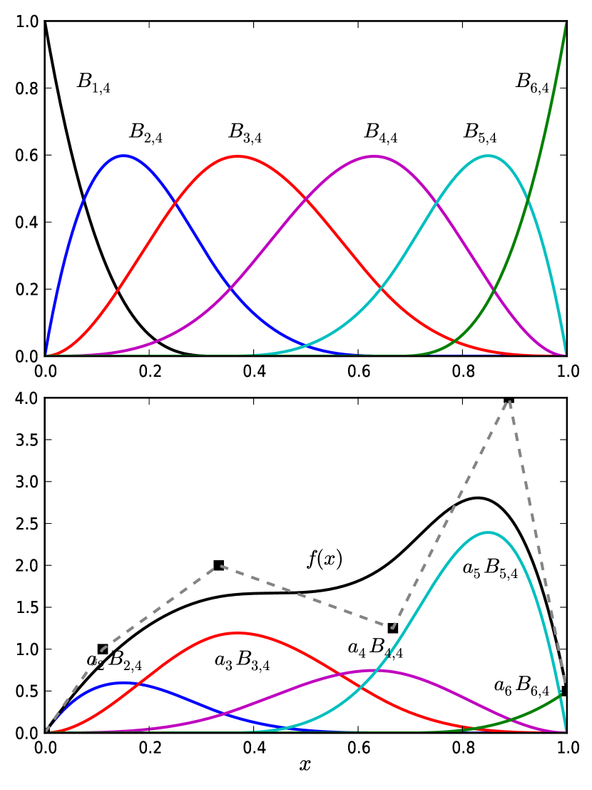
Figure 1: Top panel: B-spline basis functions of order $k=4$ (polynomial degree $=3$) for the uniform knot sequence $[0,0,0,0,1/3,2/3,1,1,1,1]$. Bottom panel: a B-spline representation of a function $f(x)=\sum_{i}a_{i}B_{i,k}(x)$ for the set of coefficients $a_{i}=\{0,1,2,1.25,4.0,0.5\}$ on the same knot sequence. The B-spline basis functions multiplied with the corresponding coefficient are also plotted. The control polygon is the dashed line, and the black squares are the positions of the control points. Due to the multiplicity of the first and last knots the function $f(x)$ attains the values of the first $a_{1}=0$ and last $a_{6}=0.5$ coefficients.

In Fig. 1 we plot (top panel) the B-spline basis functions $B_{i,4}(x)$ (order $k=4$, polynomial of degree $k-1=3$) for the knot sequence $\xi_{i}=[0,0,0,0,1/3,2/3,1,1,1,1]$. The dimension of the knot vector is $\dim(\mn@boldsymbol{\xi})=10$, thus according to our definition $m=9$. Then there exist $n=m+1-k=6$ linearly independent bases of order $k=4$.

3.2 B-spline Curves

A B-spline curve in 2 dimensional space is the linear combination of some $n$ constant vector coefficients $\mathbf{c}_{i}$ with the B-spline basis functions $B_{i,k}$:

$$\mathbf{P}(x)=\sum_{i=1}^{n}\mathbf{c}_{i}B_{i,k}(x)$$ (7)

$\mathbf{P}(x)$ is the position vector that traces the curve parametrized by $x$. The position vectors $\mathbf{c}_{i}$ are called control points. They define the $n$ vertices of an open polygon which is called the control polygon. This control polygon defines the shape of the B-spline curve. By adjusting the control points, the curve acquires a different geometric shape.

We state without proof two very important properties of B-spline curves:

1. An important class of B-spline curves is the one for which the first $\xi_{0}$ and last $\xi_{m}$ knots have multiplicity $p$ equal to the order $k$ of the B-spline curve. It can be proved then, that the B-spline curve passes from the first $\left(\mathbf{c}_{1}=\mathbf{P}(\xi_{0})\right)$ and last $\left(\mathbf{c}_{n}=\mathbf{P}(\xi_{m})\right)$ points of the control polygon. This is crucial for our subsequent analysis since, if from some physical considerations we know the boundary conditions at the beginning or the end of a curve, then we know the coordinates of the first $\mathbf{c}_{1}$ or last $\mathbf{c}_{m}$ control points. This property in combination with the smooth behaviour of B-spline curves proves to be a severe restriction on our models. All curves we are going to consider have multiplicity $p=k$ in the first and last knots.

2. Having defined a knot vector $\mn@boldsymbol{\xi}$ and knowing the control points $\mathbf{c}_{i}$, then these completely determine the tangent curve curve $\mathbf{T}(x)$ of $\mathbf{P}(x)$. This is simply:

   $$\mathbf{T}(x)=\frac{d\mathbf{P}(x)}{dx}=\sum_{i=1}^{n}\mathbf{c}_{i}\frac{dB_{i,k}(x)}{dx}$$ (8)

   Since the basis functions $B_{i,k}(x)$ are known polynomial functions, so are their derivatives. Thus, the control points $\mathbf{c}_{i}$ define the curve and all of its derivatives. This is a remarkable property for our needs in dynamical analysis. Each time we encounter an unknown function that participates in some differential equation, then by using a B-spline representation of the function we no longer need to solve the differential equation. Instead, we simply need to calculate the unknown coefficients $a_{i}$ through some algebraic process. We shall see later that this property removes the complexity in the SSJE of having to calculate $\sigma_{rr}^{2}$ and its first derivative.

3.3 B-spline Functions

A B-spline function is the linear combination of some constant coefficients $a_{i}$ with the B-spline basis functions $B_{i,k}(x)$:

$$f(x)=\sum_{i=1}^{n}a_{i}B_{i,k}(x)$$ (9)

The properties of B-spline curves are transfered also to B-spline functions:

1. For a B-spline function $f(x)=\sum_{i=1}^{n}a_{i}B_{i,k}(x)$ defined on some knot vector, if the multiplicity of the first $\xi_{0}$ and last $\xi_{m}$ knot is equal to the B-spline basis order $k$ then $f(\xi_{0})=a_{1}$ and $f(\xi_{m})=a_{n}$.

2. For a given knot sequence $\xi_{0},\ldots,\xi_{m}$, the constant coefficients $a_{i}$ uniquely determine the function $f(x)$ and all of its derivatives.

An example of a B-spline function is given in the bottom panel of Fig. 1. We define our function with the use of the B-spline basis functions $B_{i,4}(x)$ that are on the top panel (order $k=4$, knot sequence $\xi_{i}=[0,0,0,0,1/3,2/3,1,1,1,1]$) and the set of coefficients $a_{i}=\{0,1,2,1.25,4.0,0.5\}$; we plot the function $f(x)=\sum_{i=1}^{6}a_{i}B_{i,4}(x)$, the weighted B-spline basis functions $a_{i}B_{i,4}(x)$ as well as the control polygon of the B-spline curve $\mathbf{P}(x)=(x,f(x))$. The coordinates of the control points are given by $\mathbf{c}_{i}=\binom{a_{i}}{\xi_{i}^{*}}$, where $\xi_{i}^{*}$ are called Greville abscissae and are not to be confused with the knot points $\xi_{i}$. These are defined as the mean position of $k-1$ consecutive knots $\xi_{i}$

$$\xi_{i}^{*}=\frac{1}{k-1}(\xi_{i}+\xi_{i+1}+\cdots+\xi_{i+k-2})$$

see Farin:2001:CSC:501891 for details.

B-spline curves and functions are used extensively in CAGD and in statistical modelling of data, whenever a smoothing model function is needed. The quality of the resulting fit depends on the order $k$ of the spline, on the distribution of knot points, and on the number of coefficients. There is no optimum choice since all of the above parameters depend on our data. We need to use model comparison for the best choices of order $k$, knot distribution and number of knot points. In general, a bad choice of all the above parameters can result in overfitting or underfitting to the data. Bayesian inference solves partially this problem by finding the model that has the optimum knot order $k$ and number of coefficients $a_{i}$. Again, there still remains the problem of optimum smoothing, since it may be the case that we have data with large errors that result in unphysical oscillatory behaviour in the functions we represent with B-spline bases. We give a solution to this in Paper II by introducing a smoothing penalty that uses information of the smoothness from ideal theoretical models.

Our goal is to use a B-spline function representation for the radial velocity dispersion $\sigma_{rr}^{2}(r)$:

$$\sigma_{rr}^{2}(r)=\sum_{i=1}^{n}a_{i}B_{i,k}(x).$$

Doing so, we recover the values of the coefficients $a_{i}$ from comparison with observational values of the line-of-sight velocity dispersion $\sigma_{los}^{2}(R)$, thus determining the anisotropy of the system in a unique way.

3.4 Choice of knot sequence

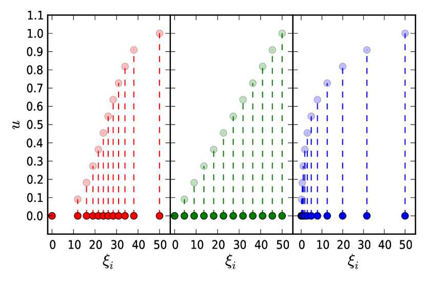
Figure 2: Various knot distributions for a B-spline basis. Left panel: Gaussian knot distribution $\xi_{i}$ around mean $\mu=25$ with $\gamma=5$. Middle panel: uniform knot distribution. Right panel: exponential knot distribution.

The distribution of knot points $\xi_{i}$ is one way to affect the geometric shape of a curve described by a B-spline function $\mathbf{P}(x)=(x,f(x))$. For our purposes we want to approximate a physical quantity, i.e. $\sigma_{rr}^{2}(r)$, with a B-spline representation. This approximation is better if we have more knot points distributed around regions where our function has greater curvature. If we have no information on where this region might be, we use a uniform distribution of knot points.

For a King mass model, we know that a critical distance from the cluster center is the King core radius $r_{c}$. It is around this point where the several functions of the model appear to have increased curvature. Therefore, we have the option of using a Gaussian knot distribution with mean $\mu=r_{c}$ and variance $\sigma=r_{t}/\gamma$, where $r_{t}$ is the tidal radius of our system. The parameter $\gamma$ regulates how close to the mean the distribution of points will be. A large value of $\gamma$ concentrates points around $r_{c}$. A value $\gamma=1$ results in an approximately uniform distribution in the interval $\xi_{i}\in[0,r_{t}]$.

Let $u$ be a uniform sequence of numbers in the interval $[0,1]$. For this sequence, the following equation gives rise to a Gaussian distribution of points around the mean $\mu$ with variance $\sigma$:

$$\xi(u)=\mu+\sqrt{2}\sigma\operatorname{erf}^{-1}\biggl{[}\operatorname{erf}\left(\frac{\mu}{\sqrt{2}\sigma}\right)(u-1)+\\ +u\operatorname{erf}\left(\frac{r_{t}-\mu}{\sqrt{2}\sigma}\right)\biggr{]}$$ (10)

Equation 10 is produced with the same methodology we use when we wish to create a random Gaussian number $\xi\in[0,r_{t}]$ from a uniform random $u\in[0,1]$.

In Fig. 2 we plot several possible choices of knot distributions. Specifically the left panel demonstrates a Gaussian distribution of points around mean $\mu=25$ with coefficient $\gamma=5$. The middle panel has a uniform distribution of knots, while the right panel is an exponential knot distribution with the majority of knots concentrated exponentially close to the origin.

3.5 The Spherically Symmetric Jeans Equation

In this section we describe how we combine the SSJE with the line-of-sight velocity dispersion $\sigma_{los}^{2}$ in order to facilitate comparison with observables. For the case of our Galaxy, where typically, one only has radial velocities, see Appendix LABEL:DLI_BSplines_MW.

In order to apply our method, we write Equations 1 and 3 in what we believe to be a much simpler form in terms of $\sigma_{rr}^{2}$ and $\sigma_{tt}^{2}$. Furthermore, we simplify the notation by setting:

$$\psi =\sigma_{rr}^{2}(r)$$ (11)

$$\phi =\sigma_{tt}^{2}(r).$$ (12)

Then the SSJE and $\sigma_{los}^{2}(R)$ in the $\psi$, $\phi$ representation are:

$$-\frac{d\Phi}{dr} =\frac{d\psi}{dr}+\left(\frac{1}{\rho}\frac{d\rho}{dr}+\frac{2}{r}\right)\psi-\frac{1}{r}\phi$$ (13)

$$\sigma_{los}^{2} =\frac{1}{\Sigma(R)}\int_{R}^{r_{t}}\frac{\rho\left[2\psi(r^{2}-R^{2})+\phi R^{2}\right]}{r\sqrt{r^{2}-R^{2}}}$$ (14)

As we shall see in section 3.6 the tidal radius $r_{t}$ of the system is defined through Poisson’s equation from $\rho(r)$ and $\Phi(r)$ and does not depend on the kinematic quantities $\sigma_{rr}^{2}$ or $\sigma_{tt}^{2}$. The problem with Equations 13 and 14 is that both functions $\psi$ and $\phi$ are unknown, and cannot be deduced from the mass density $\rho(r)$ or the potential $\Phi(r)$ of the system. Moreover, $\psi$ participates also with its first derivative, making the problem even more complex.

We are going to consider the expansion of $\psi(r)$ in a B-spline basis function of order $k$. That is:

$$\psi(r)=\sum_{i=1}^{N_{\text{coeffs}}}a_{i}B_{i,k}(r)$$ (15)

where $B_{i,k}(r)$ are known B-spline basis functions. Then the derivative of this function is merely:

$$\psi^{(1)}(r)=\sum_{i=1}^{N_{\text{coeffs}}}a_{i}B^{(1)}_{i,k}(r)$$ (16)

where $\psi^{(1)}(r)=d\psi/dr$ and $B^{(1)}_{i,k}(r)=dB_{i,k}(r)/dr$. That is, the derivative of $\psi$ depends on the same unknown coefficients $a_{i}$ but is expanded in a new set of basis functions $B_{i,k}^{(1)}(r)$. This removes the complexity of not knowing the derivative of $\psi(r)$. Substituting $\phi$ from Equation 13 in the integrand of $\sigma_{los}^{2}$ (Equation 14) yields:

$$\sigma_{los}^{2}=\frac{1}{\Sigma(R)}\int_{R}^{r_{t}}\frac{\left(2r\rho+\rho^{(1)}R^{2}\right)\psi+\rho R^{2}\psi^{(1)}}{\sqrt{r^{2}-R^{2}}}dr\\ +\frac{1}{\Sigma(R)}\int_{R}^{r_{t}}\frac{\rho R^{2}}{\sqrt{r^{2}-R^{2}}}\frac{d\Phi}{dr}dr$$ (17)

where $\rho^{(1)}=d\rho(r)/dr$. Now the line-of-sight velocity dispersion depends on the mass density of the system, the potential and the unknown function $\psi$ along with its first derivative $\psi^{(1)}$. Using the basis expansion (Equations 15 and 16) yields:

$$\sigma_{los}^{2}=\\ \sum_{i}a_{i}\frac{1}{\Sigma(R)}\int_{R}^{r_{t}}\frac{\left(2r\rho+\rho^{(1)}R^{2}\right)B_{i,k}(r)+\rho R^{2}B_{i,k}^{(1)}(r)}{\sqrt{r^{2}-R^{2}}}dr\\ +\frac{1}{\Sigma(R)}\int_{R}^{r_{t}}\frac{\rho R^{2}}{\sqrt{r^{2}-R^{2}}}\frac{d\Phi}{dr}dr$$ (18)

We define the following functions:

$$I_{i}(R) \equiv\frac{1}{\Sigma(R)}\int_{R}^{r_{t}}\frac{\left(2r\rho+\rho^{(1)}R^{2}\right)B_{i,k}(r)+\rho R^{2}B_{i,k}^{(1)}(r)}{\sqrt{r^{2}-R^{2}}}$$ (19)

$$C(R) \equiv\frac{1}{\Sigma(R)}\int_{R}^{r_{t}}\frac{\rho(r)R^{2}}{\sqrt{r^{2}-R^{2}}}\frac{d\Phi(r)}{dr}$$ (20)

Then, the value of $\sigma_{los}^{2}(R)$ is given by:

$$\sigma_{los}^{2}(R)=\sum_{i}a_{i}I_{i}(R)+C(R)$$ (21)

Comparing the line-of-sight velocity dispersion $\sigma_{los}^{2}$ with observables we can determine the marginalized distributions of the unknown coefficients $a_{i}$ as well as the defining parameters of the mass model. That is, although we cannot know the velocity profile of the cluster from its mass density $\rho(r)$ or the potential, we may allow this to be deduced from the observables. Knowledge of $a_{i}$ is equivalent to knowledge of $\sigma_{rr}^{2}\equiv\psi$ and $\sigma_{tt}^{2}\equiv\phi$.

The coefficients $a_{i}$ cannot take arbitrary values. One restriction to be applied is that both $\psi\equiv\sigma_{rr}^{2}$ and $\phi$ functions (Eq. 13) are positive. Moreover, the function $\psi$, must equal zero at $r=r_{t}$, the tidal radius of the system, and we assume that $\phi$ and $\sigma_{los}^{2}$ are also zero at $r=r_{t}$. This last condition, combined with the smoothness of B-spline functions, imposes a severe restriction on the possible values of $a_{i}$. The result is well-defined curves with small error bars. We will see later that closer to $r_{t}$ the variance of the $a_{i}$ coefficients becomes small.

From Equations 19 and 20, we see that $C(r_{t})=I_{i}(r_{t})=0$ by definition, since the lower and upper limits of the integrals coincide. Then we must impose an ad hoc restriction that $\sigma_{los}^{2}\to 0$ as $r\to r_{t}$. This is easily achieved by adding an artificial data point very close to $r_{t}$ in which we demand $\sigma_{los}^{2}\approx 0$ within some very small error.

3.6 Dynamical Models

In the following sections we will reconstruct from synthetic data the kinematic profile of a stellar system in equilibrium, i.e. $\sigma_{rr}^{2}$ and $\sigma_{los}^{2}$ (once $\sigma_{rr}^{2}$ is known, $\sigma_{tt}^{2}$ can be found from the SSJE). We will assume that the stellar mass content of this system is described by a King-model mass density $\rho(r)$. In the current contribution this is the only mass density we are going to consider. For systems that contain also a dark matter component, see Paper II.

For a full description of King models the reader should consult 1966AJ.....71...64K and 2008gady.book.....B. Here we give for reference the functional forms we used. A King model is defined through its distribution function:

$$f(\mathcal{E}) =\begin{cases}\frac{f_{0}}{(2\pi\sigma^{2})^{3/2}}\left(e^{-\mathcal{E}/\sigma^{2}}-1\right)&\mathcal{E}<0\\ 0&\mathcal{E}\geq 0\end{cases}$$ (22)

where $f_{0}$ and $\sigma$, are parameters to be determined from Bayesian likelihood methods.

Let $r_{t}$ denote the tidal radius of the system, i.e. a position beyond which the mass density and all physical quantities of the system vanish. If $\Phi(r)$ is the potential, by making use of an arbitrary additive constant to its definition, we may define as a new potential the difference: $\Psi=\Phi(r)-\Phi(r_{t})$; now $\Psi$ vanishes at the tidal radius. Furthermore, in order to simplify our calculations, we introduce the transformation: $w=-\Psi(r)/\sigma^{2}$. Then:

$$\mathcal{E}=\frac{v_{r}^{2}+v_{t}^{2}}{2}-2\sigma^{2}w(r)$$ (23)

The mass density of the system $\rho(r,w)$ can be calculated analytically with the use of Computer Algebra Systems (e.g. Maxima, Mathematica, Maple), as functions of radius $r$ and “potential” $w(r)$ :

$$\rho(r,w)=4\pi\int_{v_{r}=0}^{\sqrt{2\sigma^{2}w}}\int_{v_{t}=0}^{\sqrt{2\sigma^{2}w-v_{r}^{2}}}f(\mathcal{E},L)v_{t}dv_{t}dv_{r}$$

$v_{r}$ is the radial component of the velocity in spherical coordinates $(v_{r},v_{\theta},v_{\phi})$ and $v_{t}^{2}=v_{\theta}^{2}+v_{\phi}^{2}$. A model is fully described once we assign values to its defining parameters and know the functional form of the “potential” $w(r)$. The latter is achieved by solving Poisson’s equation numerically. To do this, we require two additional assumptions at $r=0$: an initial value for the potential $w_{0}$ and the equilibrium condition $\frac{dw}{dr}\bigr{|}_{r=0}=0$.

Instead of $(f_{0},\sigma)$ it is very convenient to use the mass core density $\rho_{0}$ and the King core radius $r_{c}$ defined by:

$$\rho_{0} =\rho\left(r,w(r)\right)\bigr{|}_{r=0}, r_{c} =\left(\frac{9\sigma^{2}}{4\pi G\rho_{0}}\right)^{1/2}$$

Then for the full description of a King model we use the following set of parameters $(w_{0},\rho_{0},r_{c})$. Using the transformed potential $w$, the Poisson equation is most conveniently written:

$$\nabla^{2}w(r) =-\frac{9}{r_{c}^{2}}\tilde{\rho}(r,w), \text{where}\quad\tilde{\rho}(r,w) =\frac{\rho(r,w)}{\rho_{0}}$$ (24)

The steps followed for a full evaluation of a King model are the following:

1. Assign initial values to parameters $(w_{0},\rho_{0},r_{c})$.

2. Subject to the initial conditions $w(r=0)=w_{0}$ and $\frac{dw}{dr}|_{r=0}=0$, solve Poisson’s equation numerically, to thus obtain $w(r)$.

3. The mass density $\rho(r)$ is fully determined upon knowledge of $w(r)$.

In the following we are going to use only the King mass density, and pretend that we do not know the kinematic quantities $\sigma_{rr}^{2}$ and $\sigma_{tt}^{2}$ as defined from the distribution function (Eq. 22).

4 Statistical Analysis

In this section we will be using standard Bayesian approaches to model fitting. The reader is directed to standard texts such as hastie01statisticallearning; sivia2006data and 2010blda.book.....G for further details.

4.1 Likelihood function

Let $\theta$ represent the vector of parameters needed to fully describe a given assumed physical model. These will be the set of defining parameters of the dynamical model, and the coefficients $a_{i}$ of the B-spline representation of $\psi\equiv\sigma_{rr}^{2}$, i.e. $\theta=(w_{0},\rho_{0},r_{c},a_{1},\ldots,a_{n-1})$. In the present paper we consider for simplicity an example with fixed mass-to-light ratio $\Upsilon=1$, therefore we do not include $\Upsilon$ as a free parameter. We emphasize however that our algorithm can treat also cases with mass-to-light ratio as a free parameter (Paper II). In the framework of Bayesian interpretation we are interested in the posterior probability distribution of these parameters. Our data set consists of kinematic $D_{K}$ and brightness $D_{B}$ data. The kinematic data set, $D_{K}$, consists of line-of-sight velocity dispersion, $\sigma_{los}^{2}$, values that can be evaluated from line-of-sight velocities, $v_{los}$, and positions, $R_{i}$, of stars. The full data set is $D=\{D_{B},D_{K}\}$ and the posterior probability of our complete data set is:

$$P(\theta|D)\propto P(\theta)\mathcal{L}(D|\theta)$$ (25)

$P(\theta)$ represents the probability of uniform prior range for each variable, i.e.:

$$P(\theta)=\prod_{i=1}^{N_{\text{params}}}\frac{1}{\Delta\theta_{i}},$$ (26)

when $\theta\in\Delta\theta_{i}$ and $0$ otherwise. $N_{\text{params}}$ represents the total number of parameters and $\Delta\theta_{i}$ the range of possible values for parameter $i$. $\mathcal{L}(D|\theta)$ is the likelihood model.

Our likelihood model must take into account both the brightness and kinematic data. Since these two datasets are mutually independent it follows that:

$$\mathcal{L}(D|\theta)=\mathcal{L}(D_{B}|\theta)\mathcal{L}(D_{K}|\theta)\equiv\mathcal{L}_{B}\cdot\mathcal{L}_{K}$$ (27)

For $\mathcal{L}_{B}$ and $\mathcal{L}_{K}$ we choose standard Gaussian distributions, i.e.:

$$\mathcal{L}_{B} =\prod_{i=1}^{N_{\text{data}}}\frac{1}{\sqrt{2\pi(\delta J_{i})^{2}}}\exp\left(-\frac{(J_{i}-\Sigma(R_{i})/\Upsilon)^{2}}{2(\delta J_{i})^{2}}\right)$$ (28)

$$\mathcal{L}_{K} =\prod_{i=1}^{N_{\text{data}}}\frac{1}{\sqrt{2\pi(\delta d_{i})^{2}}}\exp\left(-\frac{(d_{i}-\sigma_{los}^{2}(R_{i}))^{2}}{2(\delta d_{i})^{2}}\right).$$ (29)

$J_{i}$ is our brightness data values, $\delta J_{i}$ the error in each value. $d_{i}$ is the line-of-sight $\sigma_{los}^{2}(R_{i})$ data value at position $R_{i}$, $\delta d_{i}$ the corresponding error. In the example presented in Section 5, the brightness $J_{i}$ and line-of-sight velocity dispersion observables $d_{i}$ are evaluated on the same positions, $R_{i}$, however this need not be the case and this does not affect the efficiency of the method.

In order to estimate the highest likelihood values of the parameters $\theta$ we employed a Markov Chain Monte Carlo (MCMC) algorithm, namely a stretch move as described in GoodmanWeare. This method has the advantage of exploring the parameter space efficiently, and the fitted parameters generally do not get stuck around local maxima of the likelihood function. This is an important feature since if there is a degeneracy in pair of $(\rho,\beta)$ values, then we must recover multimodal distributions for the parameters $a_{i}$. Our MCMC walks were run for sufficient autocorrelation time, so as to ensure that the distributions of parameters were stabilized around certain values.

Two important remarks need to be made here: due to the complexity of the problem, if we increase the number of $a_{i}$ coefficients to more than 15, the autocorrelation time becomes very large. There were cases in our initial trial runs where we needed to run our MCMC for up to $10^{7}$ points, because the chains were converging very slowly. The behaviour of the chains is different than in standard parameter estimates of functions. Specifically the values tend to concentrate at some region quite fast, and then this whole region oscillates slowly until it is eventually stabilized. In general, for our models, we run our MCMC for approximately $2-4\times 10^{6}$ points, and this was sufficient. However we did not need to use more than $7-12$ unknown $a_{i}$ coefficients.

4.2 Bayesian Model Selection

Table 1: Jeffreys table

$\ln\left(\frac{p(M_{1})}{p(M_{2})}\right)$	$\frac{p(M_{1})}{p(M_{2})}$	Strength of evidence
$<0$	$<1$	negative (supports M2)
0 to $1.16$	1 to 3.2	barely worth mentioning
$1.16$ to $2.3$	3.2 to 10	positive
$2.3$ to $4.6$	10 to 100	strong
$>4.6$	$>100$	very strong - decisive

Jeffreys table is a quantitative table for the comparison of two competing models $M_{1}$ and $M_{2}$.

In our present description we use Bayesian model selection (gelman2003bayesian; 2010blda.book.....G) and Nested Sampling (Skilling, hereafter JS04), a method for estimating the evidence for a given likelihood model. For completeness, we give a short introduction to these methods.

Let $M_{i}$ represent each of the models used in our analysis (e.g. $M_{1}\equiv$ King mass density, with specific number $n$ of coefficients $a_{i}$, order of B-spline $k$ and knot distribution). Furthermore let $I=M_{1}+\cdots+M_{n}$ represent our hypothesis, that at least one of the models is correct. Summation indicates logical “or”. Let $\theta$ represent the total number of parameters for each model and $D$ our data set. According to Bayes theorem the probability of the model parameters $\theta$ given the data set of values is:

$$p(\theta|D,M_{i},I)=\frac{p(\theta|M_{i},I)\mathcal{L}(D|\theta,M_{i},I)}{p(D|M_{i},I)}.$$ (30)

$p(\theta|M_{i},I)$ is the prior information on the parameters, $\mathcal{L}(D|\theta,M_{i},I)$ is the likelihood as defined in Equation 27 and $p(D|M_{i},I)$ is the normalization constant for the model $M_{i}$ under consideration. This constant plays an important role for model selection. Marginalizing over all parameters, for the set of competing hypothesis, the probability of a model given the data is:

$$p(M_{i}|D,I)=\frac{p(M_{i}|I)p(D|M_{i},I)}{p(D|I)}$$ (31)

Our level of ignorance of model choice suggests that $p(M_{i}|I)=p(M_{j}|I)$ for any $i,j$ combination (all models are equiprobable). Hence the relative ratio of probabilities of two models is:

$$\frac{p(M_{i}|D,I)}{p(M_{j}|D,I)}=\frac{p(M_{i}|I)p(D|M_{i},I)}{p(M_{j}|I)p(D|M_{j},I)}=\frac{p(D|M_{i},I)}{p(D|M_{j},I)}=O_{ij}$$ (32)

$O_{ij}$ is defined as the odds ratio, and it quantifies the comparison of two competing models for the description of observables. $p(D|I)$ is the normalization constant that does not participate in our calculations each time we compute the relative ratio of two models. A measure for model selection is given by Jeffreys table (Table 1). It quantifies the relative ratio of probabilities $p(M_{1})/p(M_{2})$ of two competing models. See Jeffreys61 and gelman2003bayesian for further details.

Nested Sampling, introduced by JS04, is an algorithm for the estimation of the normalization parameter $p(D|M_{i},I)$. Following his terminology, the evidence $Z_{i}$ of model $M_{i}$ is given by:

$$Z_{i}=p(D|M_{i},I)=\int p(\theta|M_{i},I)\mathcal{L}(D|\theta,M_{i},I)d\theta$$ (33)

and corresponds to the normalization constant $p(D|M_{i},I)$. Making use of the prior mass $dX=p(\theta|M_{i},I)d\theta$, an effective parameter transformation from $\dim(\theta)=n$ to $\dim(X)=1$, the above integral is simplified:

$$Z_{i}=\int_{0}^{1}\tilde{\mathcal{L}}(D|X)dX$$ (34)

In order to estimate this quantity and perform model selection we use MultiNest (2008MNRAS.384..449F; 2009MNRAS.398.1601F). This algorithm is designed for effective calculation of Bayesian evidence based on Skilling’s algorithm. It gives consistent results even in the case of multimodal likelihood functions.

5 Example: Isotropic system with King mass density

In this section we are going to reconstruct the kinematic profile of an isotropic King model ($\beta(r)=0$). For the notation of the total number $n$ of unknown coefficients $a_{i}$ we use the following scheme: based on the restriction that all the quantities that describe the cluster must be zero at the tidal radius, the final coefficient will be $a_{n}=0$. This extra coefficient does not go into the likelihood analysis, hence we break the total number of coefficients to the sum of unknowns plus one which represents this last coefficient. We use this notation in the figure captions and in Table 2 where we list the Bayesian evidence.

Table 2: Bayesian Evidence for isotropic system with King mass model

Order	Number of coefficients $n$	$\ln Z\pm\delta(\ln Z)$
$k=4$	$n=5+1$	$-50.15\pm 0.19$
	$n=6+1$	$-41.19\pm 0.20$
$k=5$	$n=5+1$	$-41.44\pm 0.20$
$k=5$	$n=6+1$	$-45.06\pm 0.20$

From left to right: first column is the order $k$ of the B-spline representation of $\psi\equiv\sigma_{rr}^{2}(r)$. Second column is the number $n$ of coefficients $a_{i}$. The third column is the value of Bayesian evidence as estimated from MultiNest. The highest value of $\ln Z$ corresponds to the most probable model.