A Generalized and Adaptive Method for Community Detection

Abstract

Complex networks represent interactions between entities. They appear in various contexts such as sociology, biology, etc., and they generally contain highly connected subgroups called communities. Community detection is a well-studied problem and most of the algorithms aim to maximize the Newman-Girvan modularity function, the most popular being the Louvain method (it is well-suited on very large graphs). However, the classical modularity has many drawbacks: we can find partitions of high quality in graphs without community structure, e.g., on random graphs; it promotes large communities. Then, we have adapted the Louvain method to other quality functions.

In this paper, we describe a generic version of the Louvain method. In particular, we give a sufficient condition to plug a quality function into it. We also show that global performance of this new version is similar to the classical Louvain algorithm, that promotes it to the best rank of the community detection algorithms.

Key words: Community detection, complex networks, Louvain method

1 Introduction

Complex networks are very common in different areas such as sociology (e.g., friendship or collaboration networks), computer science (e.g., networks of computers), biology (e.g., gene regulatory networks or neural networks). These networks are often modeled using the graph formalism which represents the interactions between a set of entities. For example, a social network can be represented by a graph whose nodes (or vertices) are individuals and links (or edges) represent a kind of social relationship.

Most complex networks exhibit a community structure, i.e. are composed of groups of highly connected nodes (e.g., groups of friends or collaborators) [21, 36]. The automatic detection of such communities has attracted much attention in recent years and many community detection algorithms have been proposed (see [19] for a survey). In most studies, the detection of communities aims at finding a partition of the nodes of the graph, i.e. any given node belongs to exactly one community, and communities are, therefore, groups of highly connected nodes and loosely connected to the rest of the graph. A classical way to assess the quality of a partition in communities is to maximize the quality function known as modularity [34], which measures the difference between the effective and the expected internal link density in communities. However, due to the intrinsic NP-hardness of linear programming with binary variables subject to the linear constraints of a partition (proved in [23] and after in [38] for the acyclic subgraph problem), modularity maximization is an NP-hard problem [11] and most algorithms use heuristics. Among the formers, one of the most efficient (both in speed and quality) is the Louvain method [7, 10], which is an hierarchical local greedy technique to maximize modularity.

While modularity (and its maximization) has gained a lot of attention in the complex networks field since it was proposed, many other quality functions have been defined in close or very different contexts, and the first notable proposition, derived from the works of Condorcet about voting consensus [16], was made by C. T. Zahn [40] in the sixties.

Given that other functions have not been studied deeply in the complex network field, we propose here a generic version of the Louvain algorithm that can be used on a large variety of criteria. To achieve this, we show that the Louvain method core is mainly independent of the underlying quality function and, therefore, that it can be generalized to many other quality functions. We also give a sufficient condition for a quality function which ensures that it can be efficiently plugged into the Louvain framework.

Our paper is organized as follows: in Sect. 2 we present the Louvain method and we point out the portions of the algorithm which are directly used for modularity maximization. In Sect. 3 we present a large variety of criteria to evaluate a partition and we show two properties of such criteria that can can be used to decide whether a criterion can be plugged into Louvain or not. In Sect. 4 we give the generic version of the Louvain algorithm and we instantiate it for another criterion. We also give a sufficient condition for a quality function to be efficiently pluggable into Louvain and give an example of a criterion which does not meet this condition but can be efficiently plugged (since the condition is not necessary). Finally, we show in Sect. 5 that the generic version of the Louvain method is very efficient for most criteria and that it can successfully replace the classical Louvain algorithm.

2 The Louvain method

The Louvain algorithm has first been introduced to find partitions of high Newman-Girvan modularity, which is the most widely used criterion to evaluate a partition of a complex network. The algorithm uses a local greedy optimization to find a local maxima of modularity, which is further enhanced with a hierarchical refinement. The local greedy optimization is described in Algorithm 1: it consists in moving nodes one by one in one of their neighboring community so as to obtain the maximal increase of modularity. Nodes can be moved several times and this procedure stops only when a local maxima is obtained, i.e. when no individual move can increase the modularity. The hierarchical refinement described in Algorithm 2 consists in building a meta-graph whose nodes are the communities found in the previous step and links represent the sum of connections between the communities (see Fig. 1 for an example). The Louvain algorithm is therefore an iteration of two sub-procedures: local optimization and meta-graph construction. It stops only when no improvement can be obtained by any of the two operations.

Several improvements of the Louvain algorithm have been proposed in the literature. These improvements are directed either towards an improvement of the time efficiency mainly by using less severe stopping criteria, or towards an improvement of the quality of the result by using refinements, such as the ones proposed in [17, 20], or an improvement of the computation time by parallelization [9]. However, we will mainly focus on the simple version of the algorithm and most refinements can be used on the generic version of Louvain.

Require: $G=(V,E,w)$ a weighted graph

Ensure: a partition $\mathcal{P}$ of $V$

Local: $increase\leftarrow\texttt{true}$

Local: $\mathcal{P}$ the current partition of $V$

begin

      

      forall the nodes $i$ do

             $\mathcal{P}[i]\leftarrow\{i\}$

             INIT$(i)$

            

      

      while $increase$ do

             $increase\leftarrow\texttt{false}$

             forall the nodes $i$ do

                   $C_{\text{old}}\leftarrow\mathcal{P}[i]$

                   REMOVE$(i,C_{\textup{old}})$

                   $\mathcal{C}\leftarrow\{\mathcal{P}[j]\mid(i,j)\in E\}\cup\{C_{\text{old}}\}$

                   $C_{\text{new}}\leftarrow\arg\max_{C\in\mathcal{C}}\{$GAIN$(i,C)\}$

                   INSERT$(i,C_{\text{new}})$

                   if $C_{\textup{old}}\neq C_{\textup{new}}$ then

                         $increase\leftarrow\texttt{true}$

                        

                  

            

      

ALGORITHM 1 One pass algorithm

Require: $G=(V,E,w)$ a weighted graph

Ensure: a partition $\mathcal{P}$ of $V$

begin

       repeat

             $\mathcal{P}\leftarrow$ONEPASS$(G)$

             $G\leftarrow$PARTITION-TO-GRAPH$(\mathcal{P},G)$

            

      until no improvement is possible

ALGORITHM 2 Louvain algorithm

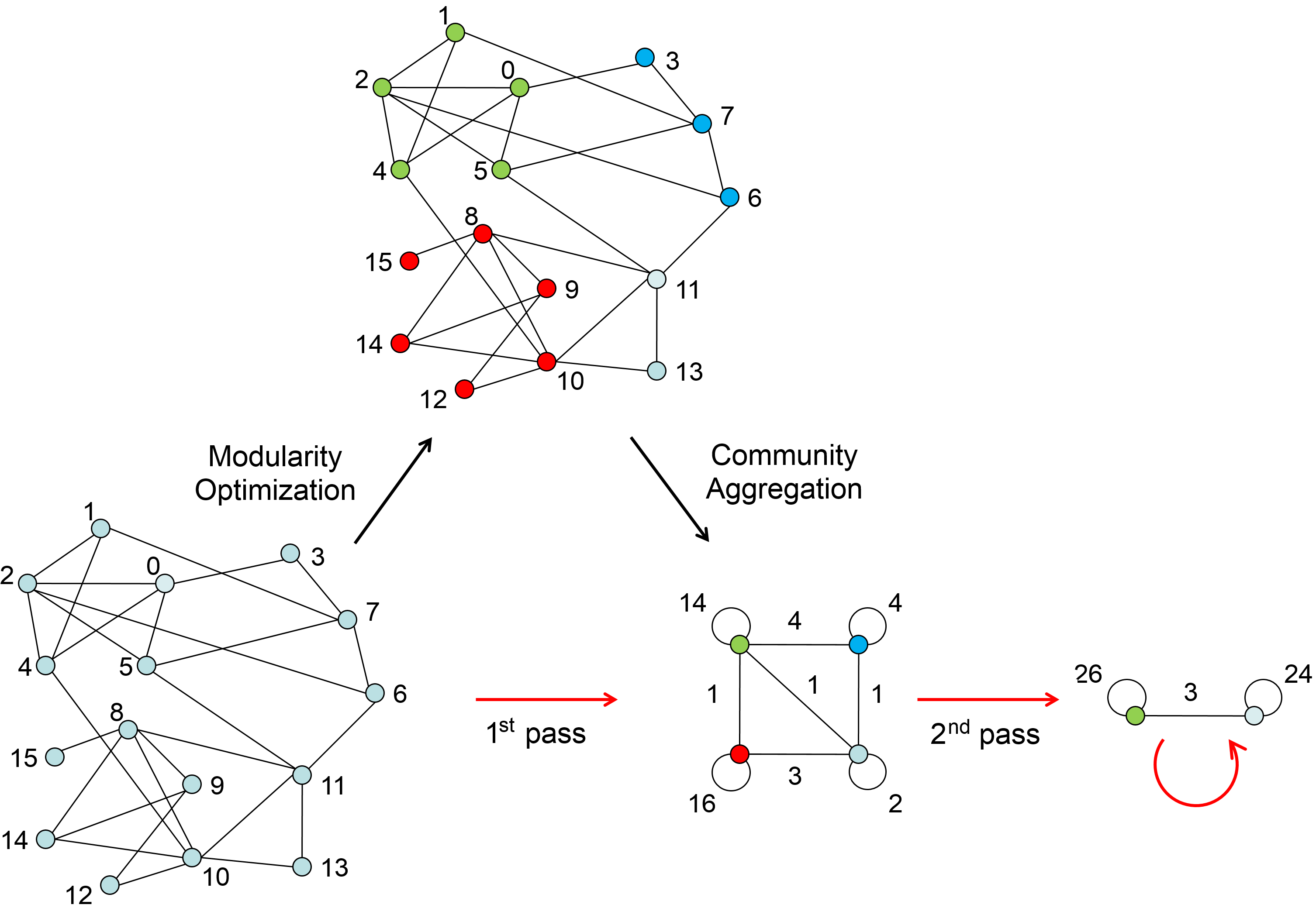
Figure 1: Louvain algorithm overview (Fig. 1 in [10])

The Louvain algorithm presented in Algorithms 1 and 2 contains several sub-functions that must be precisely defined and are strongly related to the Newman-Girvan modularity function to be optimized. Basically, one must define functions to remove (resp. insert) a node from (resp. in) a community and update all the information needed by the algorithm, and a function to compute the gain (or loss) in the value of modularity when a node is moved in a given community.

For the classical Louvain method, we give the four functions in Algorithm 3. These functions have been originally described in [10] and later in [7]. We precise here that

$$d_{w}(i,C) = \sum_{j\in C}w_{ij}\enspace,$$ (1)

with $w_{ij}$ the link weight between nodes $i$ and $j$. They are based on the use of two vectors, in and tot, which indicate, for each community, the number of intern and total links. These vectors are updated at each insertion or removal and are used to compute the modularity gain for each move. Note that the in vector is not useful since the gain in modularity when a node is moved to community $C$ can be written in a more compact form as follows

$$d_{w}(i,C)-\frac{d_{i}\cdot\textsf{tot}[C]}{2m}\enspace,$$ (2)

with $d_{i}=\sum_{j\mid(i,j)\in E}w_{ij}$ the weighted degree of node $i$ and $2m=\sum_{i\in V}d_{i}$; but it is necessary to compute the complete quality of the graph partition.

INIT$(i)$:

 begin

       $\textsf{in}[i]\leftarrow w_{ii}$

       $\textsf{tot}[i]\leftarrow d_{i}$

      

REMOVE$(i,C)$:

 begin

       $\textsf{in}[C]\leftarrow\textsf{in}[C]-2\cdot d_{w}(i,C)-w_{ii}$

       $\textsf{tot}[C]\leftarrow\textsf{tot}[C]-d_{i}$

       $\mathcal{P}[i]\leftarrow\emptyset$

      

INSERT$(i,C)$:

 begin

       $\textsf{in}[C]\leftarrow\textsf{in}[C]+2\cdot d_{w}(i,C)+w_{ii}$

       $\textsf{tot}[C]\leftarrow\textsf{tot}[C]+d_{i}$

       $\mathcal{P}[i]\leftarrow C$

      

GAIN$(i,C)$:

 begin

       return $\displaystyle\left[\frac{\textsf{in}[C]+2\cdot d_{w}(i,C)}{2m}-\left(\frac{\textsf{tot}[C]+d_{i}}{2m}\right)^{2}\right]-\left[\frac{\textsf{in}[C]}{2m}-\left(\frac{\textsf{tot}[C]}{2m}\right)^{2}-\left(\frac{d_{i}}{2m}\right)^{2}\right]$

ALGORITHM 3 Functions for the Newman-Girvan modularity

These four functions can be designed for other criteria, that we will show in Sect. 4. Before that, we will present in Sect. 3 some other criteria for graph clustering.

3 Some Criteria for Graph Clustering

Graph clustering criteria depend strongly on the meaning given to the notion of community. In the last few years, various modularization criteria have been defined in different fields, each one having its own definition of community. Although different, all definitions have something in common: dense connections within communities and only sparse connections between communities.

In this section, we present different modularization criteria in Relational coding; this notation will help us to compare those criteria on the same basis.

Since a graph represents relations between objects belonging to the same set, therefore, a non-oriented and non-weighted graph $G=(V,E)$, with $n=|V|$ nodes and $m=|E|$ links, is a binary symmetric relation on its set of nodes $V$ represented by its adjacency matrix A, whose general term is defined as

$$a_{ij}=\begin{cases}1&\text{if there exists an link between $i$ and $j$ $\forall(i,j)\in V\times V$,}\\ 0&\text{otherwise.}\end{cases}$$ (3)

In the case of a weighted graph $G=(V,E,w)$, the adjacency matrix A will be denoted W. The general term of this matrix, $w_{ij}$, represents the weight of the edge linking nodes $i$ and $j$.

Partitioning a graph implies to define an equivalence relation on the set of nodes $V$, that means a symmetric, reflexive and transitive relation. Mathematically, an equivalence relation is represented by a square matrix X whose entries are defined as

$$x_{ij}=\begin{cases}1&\text{if node $i$ and node $j$ are in the same community $\forall(i,j)\in V\times V$,}\\ 0&\text{otherwise.}\end{cases}$$ (4)

Modularizing a graph implies to define X as close as possible to A. A modularity criterion is a function which measures either a similarity or a distance between A and X. Therefore, the problem of modularization can be written as a function to optimize (minimize if the function represents a distance or maximize if the function represents a similarity). So, we have

$$\max_{X}\leavevmode\nobreak\ \text{ or }\leavevmode\nobreak\ \min_{X}F(X)\enspace,$$ (5)

subject to the constraints of an equivalence relation:

$$x_{ij}\in\left\{0,1\right\}$$ Binary

$$x_{ii}=1 \forall i$$ Reflexivity

$$x_{ij}-x_{ji}=0 \forall(i,j)$$ Symmetry

$$x_{ij}+x_{jk}-x_{ik}\leq 1 \forall(i,j,k)$$ Transitivity

We define as well $\bar{\textbf{X}}$ and $\bar{\textbf{A}}$ as the inverse relation of X and A respectively. Their entries are defined as $\bar{x}_{ij}=1-x_{ij}$ and $\bar{a}_{ij}=1-a_{ij}$ respectively. In the case of a weighted graph, the general term of the matrix $\bar{\textbf{W}}$ is calculated as follows: $\bar{w}_{ij}=\mathcal{W}-w_{ij}$, where $\mathcal{W}=\max_{(i,j)\in E}\{w_{ij}\}$.

We distinguish the criteria according to the properties they verify. We consider two properties: linearity and separability. The relational codings of these properties are shown in Table 1.

Table 1: Properties verified by modularity criteria^a

The criterion has the property	If it can be written as
Linearity	$\displaystyle{F(X)\leavevmode\nobreak\ =\leavevmode\nobreak\ \sum_{i,j\in V}\phi(a_{ij})x_{ij}+K}$
Separability	$\displaystyle{F(X)\leavevmode\nobreak\ =\leavevmode\nobreak\ \sum_{i,j\in V}\phi(a_{ij})\psi(x_{ij})+K}$

^aWe use $K$ to denote any constant depending only on the original data.

According to Table 1, the property of linearity entails that the criterion is a linear function of X. The function $\phi(a_{ij})$ depends only on the original data (i.e. the adjacency matrix). $\psi(x_{ij})$ is a function of the unknown variable $x_{ij}$. The property of separability implies that the criterion can be written as a scalar product of two vectors, the first one depending only upon the original data and the second one depending upon the unknown variable. Consequently, every linear criterion is separable.

3.1 Linear Criteria (and Separable)

The Relational coding of all linear criteria is given in Table 2. For each criterion, the optimal partition is found without fixing in advance the optimal number of clusters (or communities) $\kappa$. Just for comparison, we added the Newman-Girvan modularity.

Criterion	Relational notation
Newman-Girvan (2004)	$\displaystyle F_{\textsc{ng}}(X)\leavevmode\nobreak\ =\leavevmode\nobreak\ \sum_{i,j\in V}\left(a_{ij}-\frac{d_{i}d_{j}}{2m}\right)x_{ij}$
Zahn-Condorcet (1785, 1964)	$\displaystyle F_{\textsc{zc}}(X)\leavevmode\nobreak\ =\leavevmode\nobreak\ \sum_{i,j\in V}a_{ij}x_{ij}+\sum_{i,j\in V}\bar{a}_{ij}\bar{x}_{ij}$
Owsiński-Zadrożny (1986)	$\displaystyle F_{\textsc{oz}}(X)\leavevmode\nobreak\ =\leavevmode\nobreak\ (1-\alpha)\sum_{i,j\in V}a_{ij}x_{ij}+\alpha\sum_{i,j\in V}\bar{a}_{ij}\bar{x}_{ij}$ with $0<\alpha<1$
Marcotorchino (1991)	$\displaystyle F_{w\textsc{c}}(X)\leavevmode\nobreak\ =\leavevmode\nobreak\ \sum_{i,j\in V}\hat{a}_{ij}x_{ij}+\sum_{i,j\in V}\bar{\hat{a}}_{ij}\bar{x}_{ij}$
Balanced Modularity (2013)	$\displaystyle{F_{\textsc{bm}}(X)\leavevmode\nobreak\ =\leavevmode\nobreak\ \sum_{i,j\in V}\left(a_{ij}-\frac{d_{i}d_{j}}{2m}\right)x_{ij}+\sum_{i,j\in V}\left(\bar{a}_{ij}-\frac{(n-d_{i})(n-d_{j})}{n^{2}-2m}\right)\bar{x}_{ij}}$
Deviation to Indetermination (2013)	$\displaystyle{F_{\textsc{di}}(X)\leavevmode\nobreak\ =\leavevmode\nobreak\ \sum_{i,j\in V}\left(a_{ij}-\frac{d_{i}}{n}-\frac{d_{j}}{n}+\frac{2m}{n^{2}}\right)x_{ij}}$
Deviation to Uniformity (2013)	$\displaystyle{F_{\textsc{du}}(X)\leavevmode\nobreak\ =\leavevmode\nobreak\ \sum_{i,j\in V}\left(a_{ij}-\frac{2m}{n^{2}}\right)x_{ij}}$

Table 2: Linear modularity functions in Relational notation

1. The Newman-Girvan criterion (2004) (see [34]): also known as modularity, its definition involves a comparison of the number of within-cluster links in a real network and the expected number of such links in a random graph (without regard to community structure).

2. The Zahn-Condorcet criterion (1785, 1964): C. T. Zahn (see [40]) was the first author who studied the problem of finding an equivalence relation X, which best “approximates” a given symmetric relation A in the sense of minimizing the distance of the symmetric difference. However, the criterion defined by Zahn is a variant of the relational Condorcet’s criterion (see [16]), introduced in his works on Voting Consensus and whose relational notation was first given by [32].

3. The Owsiński-Zadrożny criterion (1986) (see [35]) is a generalization of Zahn-Condorcet’s function. It is more flexible because it contains a parameter $\alpha$ which allows the user, according to the context, to define the minimal percentage $\alpha$ of required within-cluster links in each community.

4. The Marcotorchino criterion (1991) (or the A-weighted Condorcet criterion): introduced in [30] (see also [25]), it is a derivation of the Zahn-Condorcet’s criterion. Instead of considering the adjacency matrix A, we consider the weighted A-matrix $\hat{\textbf{A}}$ and its complementary $\bar{\hat{\textbf{A}}}$, which are defined as

   $$\hat{a}_{ij}\leavevmode\nobreak\ =\leavevmode\nobreak\ \frac{2a_{ij}}{d_{i}+d_{j}}\quad\text{and}\quad\bar{\hat{a}}_{ij}\leavevmode\nobreak\ =\leavevmode\nobreak\ \frac{\hat{a}_{ii}+\hat{a}_{jj}}{2}-\hat{a}_{ij}\enspace,$$ (6)

   where $d_{i}=\sum_{j\in V}a_{ij}$ is the degree of node $i$. If the graph does not contain loops, the optimization of this criterion groups all nodes together. Therefore, before adapting this modularity function, we must add self-loops to all nodes of the graph. Moreover, the use of this criterion is limited to non-weighted graphs.

5. The Balanced Modularity criterion (2013): introduced first in [14], it is a balanced version of the Newman-Girvan modularity. In fact, it was constructed by adding to the Newman-Girvan modularity a term taking into account the absence of links $\bar{\textbf{A}}$.

6. The Deviation to Indetermination criterion (2013): analogously to Newman-Girvan function, which maximizes the deviation to the independence structure, this index maximizes the deviation to the indetermination structure (see [26], [5] and [31]).

7. The Deviation to Uniformity criterion (2013): proposed in [13], this criterion maximizes the deviation to the uniformity structure. It compares the number of within-cluster edges in the real graph and the expected number of such edges in a random graph where edges are uniformly distributed, thus all the nodes have the same degree equal to the average degree of the graph. We can compare such a network to grid or a lattice graph with no community structure.

We can see from Table 2 that all the criteria can be turned into the general form

$$F(X)\leavevmode\nobreak\ =\leavevmode\nobreak\ \sum_{i,j\in V}\left(\phi(a_{ij})x_{ij}+\bar{\phi}(\bar{a}_{ij})\bar{x}_{ij}\right)\enspace,$$ (7)

where $\phi$ and $\bar{\phi}$ are functions of the original data (in some cases, we have $\bar{\phi}(.)\leavevmode\nobreak\ =\leavevmode\nobreak\ 0$: for instance, this is the case of the Deviation to Indetermination index). From (7) and the definition of $\bar{\textbf{X}}$, we can infer that every linear criterion can be written as

$$F(X)\leavevmode\nobreak\ =\leavevmode\nobreak\ \sum_{i,j\in V}\left(\phi(a_{ij})-\bar{\phi}(\bar{a}_{ij})\right)x_{ij}+K\enspace.$$ (8)

As the unknown variable $x_{ij}$ is null if $i$ and $j$ are not in the same community, (8) allows to evaluate the function by summing up terms depending only on intra-cluster properties. Furthermore, this expression demonstrates that every linear criterion is separable.

3.2 Non-Linear Criteria

These criteria are non-linear functions of the unknown variable X; their expressions are shown in Table 3. We can deduce from this table that all criteria are separable, except the Shi-Malik function (also known as normalized cuts criterion).

Criterion	Relational notation
Profile Difference (1976)	$\displaystyle{F_{\textsc{pd}}(X)\leavevmode\nobreak\ =\leavevmode\nobreak\ 2\sum_{i,j\in V}\hat{a}_{ij}\hat{x}_{ij}-\kappa-\sum_{i,j\in V}\hat{a}_{ij}^{2}}$
Mancoridis-Gansner (1998)	$\displaystyle F_{\textsc{mg}}(X)\leavevmode\nobreak\ =\leavevmode\nobreak\ \frac{1}{\kappa}\sum_{i,j\in V}\frac{a_{ij}x_{ij}}{|C_{[i]}|\cdot|C_{[j]}|}+\frac{1}{\kappa(\kappa-1)}\sum_{i,j\in V}\frac{\bar{a}_{ij}\bar{x}_{ij}}{|C_{[i]}|\cdot|C_{[j]}|}\quad$ with $\kappa>1$
Michalski-Decaestecker (1983)	$\displaystyle F_{\textsc{md}}(X)\leavevmode\nobreak\ =\leavevmode\nobreak\ \sum_{i,j\in V}a_{ij}\hat{x}_{ij}+\sum_{i,j\in V}\bar{a}_{ij}\bar{\hat{x}}_{ij}$
Shi-Malik (2000)	$\displaystyle{F_{\textsc{sm}}(X)\leavevmode\nobreak\ =\leavevmode\nobreak\ \sum_{i,j\in V}\frac{a_{ij}\bar{x}_{ij}}{\sum_{k\in V}d_{k}x_{ik}}}$
Michalski-Goldberg (2012)	$\displaystyle{F_{\textsc{g}}(X)\leavevmode\nobreak\ =\leavevmode\nobreak\ \sum_{i,j\in V}a_{ij}\hat{x}_{ij}}$

Table 3: Non-linear criteria

1. The Profile Difference criterion (1976): introduced as a contingency measure of the distance between two partitions (see [12] and [8]), it minimizes a least square function: the squared Frobenius norm of the difference between the matrices $\hat{\textbf{A}}$ and the weighted X-matrix $\hat{\textbf{X}}$, defined as

   $$\hat{x}_{ij}\leavevmode\nobreak\ =\leavevmode\nobreak\ \frac{2x_{ij}}{|C_{[i]}|+|C_{[j]}|}\quad\text{and}\quad\bar{\hat{x}}_{ij}\leavevmode\nobreak\ =\leavevmode\nobreak\ \frac{\hat{x}_{ii}+\hat{x}_{jj}}{2}-\hat{x}_{ij}\enspace,$$ (9)

   with $|C_{[i]}|$ the size of the community containing the node $i$. The original expression of this criterion is given in relational terms by

   $$F_{\textsc{pd}}(X) = ||\hat{\textbf{A}}-\hat{\textbf{X}}||^{2}\leavevmode\nobreak\ =\leavevmode\nobreak\ \sum_{i,j\in V}\left(\hat{a}_{ij}-\hat{x}_{ij}\right)^{2}\enspace.$$ (10)

   Since X represents an equivalence relation, we have

   $$\hat{x}_{ij} = \frac{x_{ij}}{|C_{[i]}|}\leavevmode\nobreak\ =\leavevmode\nobreak\ \frac{x_{ij}}{|C_{[j]}|}\enspace.$$ (11)

   Therefore, minimizing this criterion is equivalent to maximize its expression given in Table 3, where $\kappa$ represents the number of communities (or clusters) of the optimal partition.

2. The Mancoridis-Gansner criterion (1998): originally introduced to recover the modular structure of a software from its source code in [28], this criterion aims simultaneously at maximizing intra-connectivity within clusters and minimizing inter-connectivity between clusters. The intra-connectivity of a cluster is calculated as the fraction of the maximum number of intra-cluster links. The inter-connectivity between two clusters is calculated as the fraction of the maximum number of inter-clusters links. Both measures, the intra-connectivity and the inter-connectivity, are normalized by the number of clusters $\kappa$ and the number of distinct pair of clusters $\frac{\kappa(\kappa-1)}{2}$.

3. The Michalski-Decaestecker criterion (1983) (or the X-weighted Condorcet criterion): introduced by [33] in Learning theory, its relational expression (given in [18]) is a derivate of Zahn-Condorcet criterion. This criterion is built up by replacing the unknown variables $x_{ij}$ with the weighted variables $\hat{x}_{ij}$. Unlike the criteria previously presented, for this one, it is necessary to fixe the number of clusters $\kappa$ in advance, otherwise, the optimal solution is trivial: each node is isolated and, therefore, there are $n$ clusters ($\kappa=n$).

4. The Shi-Malik criterion (2000) (or normalized cuts: see [37]): this function is of type min-cut, a type of criterion which minimizes the number of inter-cluster links (better known as cut edges) or a function of this number. The Shi-Malik criterion minimizes the cut edges as a fraction of the total link connections to all the nodes in the graph. If the number of clusters is not fixed in advance, minimizing the cut edges turns out to group all the nodes together. Hence, without fixing in advance $\kappa$, the optimal solution is trivial since all the nodes are clustered together.

5. The Michalski-Goldberg criterion (2012): (see  [22]): this function maximizes the density of edges in each community. Thus, for each cluster, the density of Goldberg is the number of within-cluster edges divided by the size of the cluster (it corresponds to the first term of the Michalski-Decaestecker criterion previously defined). It has been already used for graph partitionning in [15].

In the next section, we will show that all the linear criteria can be plugged easily into the Louvain method, i.e. we can write the three specific functions to insert (resp. remove) a node into (resp. from) a community and compute efficiently (i.e. just by re-computing locally the quality function for the community considered) the gain obtained when a node is moved in a given community.

4 A Generic Version of Louvain Algorithm

Algorithms 1 and 2 page 1 already give the generic version of Louvain algorithm. Indeed, this local optimization heuristic can be easily adapted to other quality functions than modularity. In fact, only the functions INIT, REMOVE, INSERT and GAIN described in Algorithm 3 are specifically designed for the Newman-Girvan modularity; but we can adapt these functions for other criteria: for example, Algorithm 4 explicits the functions for the Zahn-Condorcet quality function, where $s_{i}$ denotes the size of (meta-)node $i$ ($\forall i\in V$, $s_{i}=1$ for the first level of Louvain algorithm) and $\textsf{s}[C]$ denotes the size of community $C$ ($\textsf{s}[C]=\sum_{i\in C}s_{i}$).

INIT$(i)$:

 begin

       $\textsf{in}[i]\leftarrow w_{ii}$

       $\textsf{s}[i]\leftarrow s_{i}$

      

REMOVE$(i,C)$:

 begin

       $\textsf{in}[C]\leftarrow\textsf{in}[C]-2\cdot d_{w}(i,C)-w_{ii}$

       $\textsf{s}[C]\leftarrow\textsf{s}[C]-s_{i}$

       $\mathcal{P}[i]\leftarrow\emptyset$

      

INSERT$(i,C)$:

 begin

       $\textsf{in}[C]\leftarrow\textsf{in}[C]+2\cdot d_{w}(i,C)+w_{ii}$

       $\textsf{s}[C]\leftarrow\textsf{s}[C]+s_{i}$

       $\mathcal{P}[i]\leftarrow C$

      

GAIN$(i,C)$:

 begin

       return $\displaystyle 2\cdot d_{w}(i,C)-\mathcal{W}\cdot s_{i}\cdot\textsf{s}[C]$

ALGORITHM 4 Functions for the Zahn-Condorcet quality function

To obtain the GAIN function described in Algorithm 4, we have to transform the Relational notation of the criterion given in Table 2 page 2.

We recall here (for the weighted case) the Relational notation of the Zahn-Condorcet criterion:

$$F_{\textsc{zc}}(X) = \sum_{i,j\in V}w_{ij}x_{ij}+\sum_{i,j\in V}\bar{w}_{ij}\bar{x}_{ij}\enspace.$$ (12)

We try to compute (12) community by community. So, we obtain

$$F_{\textsc{zc}}(X) = \sum_{i,j\in V}\big{(}w_{ij}x_{ij}+(\mathcal{W}-w_{ij})(1-x_{ij})\big{)}$$

$$= \sum_{i,j\in V}(2w_{ij}x_{ij}+\mathcal{W}-\mathcal{W}x_{ij}-w_{ij})$$

$$= \sum_{i,j\in V}\big{(}(2w_{ij}-\mathcal{W})x_{ij}+\mathcal{W}-w_{ij}\big{)}$$

$$= \sum_{i,j\in V}(2w_{ij}-\mathcal{W})x_{ij}+\mathcal{W}\cdot n^{2}-2m\enspace,$$

where $2m=\sum_{i,j\in V}w_{ij}$ for a weighted graph.

Now, given a partition $\mathcal{P}$ in more than two communities, $\sum_{i,j\in V}w_{ij}x_{ij}$ can be turned to $\sum_{C\in\mathcal{P}}\textsf{in}[C]$ and $\sum_{i,j\in V}x_{ij}$ can be turned to $\sum_{C\in\mathcal{P}}\textsf{s}[C]^{2}$. Thus, we obtain

$$F_{\textsc{zc}}(\mathcal{P}) = \sum_{C\in\mathcal{P}}(2\cdot\textsf{in}[C]-\mathcal{W}\cdot\textsf{s}[C]^{2})+\mathcal{W}\cdot n^{2}-2m\enspace.$$ (13)

Finally, we can easily deduce from (13) the gain computation formula given in Algorithm 4, by reducing the following equation:

$$\left[2(\textsf{in}[C]+2\cdot d_{w}(i,C))-\mathcal{W}(\textsf{s}[C]+s_{i})^{2}\right]-\left[2\cdot\textsf{in}[C]-\mathcal{W}\cdot\textsf{s}[C]^{2}-\mathcal{W}\cdot s_{i}^{2}\right]\enspace.$$ (14)

Clearly, for the Zahn-Condorcet quality function, all the other communities $C^{\prime}\in(\mathcal{P}\setminus\{C\})$ are not impacted by the addition of $i$ to $C$ (i.e. their vectors in and s are not modified). Indeed, we can compute the gain to add any node $i$ to any community $C$ locally, i.e. without impacting the other communities. This is due to the fact that this criterion is linear, which is not the case for all the criteria.

We now show that all linear criteria can be integrated efficiently to Louvain.

4.1 A Sufficient Condition to Integrate Efficiently any Criterion to Louvain

The computation power of Louvain algorithm is clearly based on the fact that, at each step, we only compute a local quality, depending only on one node and one community: the Louvain method would not be so powerful if we had to compute the global quality of the partition at each step. Hence, for each criterion we want to integrate to Louvain, we have to express it locally, i.e. only for one node and one community. But how (and when) can we do that?

Let $F$ be any quality function. As we have explained in Sect. 3, this function depends on the weighted adjacency matrix of the graph W and the unknown variable X. If $F$ is a linear function of X, then, $F$ can be computed by summing products for each $(i,j)\in V\times V$. Therefore, we are able to compute $F$ only for one part of W and X, that can easily correspond to one community.

So, any quality function that verifies linearity can be implemented efficiently in the Louvain framework.

This condition is sufficient, but not necessary. Indeed, several quality functions are not linear but separable (i.e. they can be written as a scalar product of a part of $\phi(\textbf{W})$ and $\psi(\textbf{X})$): the fact that they can be efficiently plugged to Louvain strongly depends on the functions $\phi$ and $\psi$ applied on W and X.

We give in Sect. 4.2 an example of a non-linear (but separable) criterion which is efficiently pluggable to Louvain.

4.2 Several non-linear criteria (but separable) can be efficiently integrated to Louvain

Algorithm 5 gives the four functions (INIT, REMOVE, INSERT and GAIN) designed for the Profile Difference criterion ($\textsf{in}^{\prime}[C]$ and $d^{\prime}_{w}(i,C)$ correspond to the $\textsf{in}[C]$ and $d_{w}(i,C)$ modified values: see explanations below).

INIT$(i)$:

 begin

       $\textsf{in}^{\prime}[i]\leftarrow\hat{w}_{ii}$

       $\textsf{s}[i]\leftarrow s_{i}$

       $\kappa=n$

      

REMOVE$(i,C)$:

 begin

       $\textsf{in}^{\prime}[C]\leftarrow\textsf{in}^{\prime}[C]-d^{\prime}_{w}(i,C)$

       $\textsf{s}[C]\leftarrow\textsf{s}[C]-s_{i}$

       if $\textsf{s}[C]=0$ then

             $\kappa\leftarrow\kappa-1$

       $\mathcal{P}[i]\leftarrow\emptyset$

      

INSERT$(i,C)$:

 begin

       $\textsf{in}^{\prime}[C]\leftarrow\textsf{in}^{\prime}[C]+d^{\prime}_{w}(i,C)$

       if $\textsf{s}[C]=0$ then

             $\kappa\leftarrow\kappa+1$

       $\textsf{s}[C]\leftarrow\textsf{s}[C]+s_{i}$

       $\mathcal{P}[i]\leftarrow C$

      

GAIN$(i,C)$:

 begin

       if $\textsf{s}[C]=0$ then

             return $\displaystyle\frac{d^{\prime}_{w}(i,C)}{s_{i}}-\frac{1}{2}$

            

      else

             return $\displaystyle\frac{\textsf{in}^{\prime}[C]+d^{\prime}_{w}(i,C)}{\textsf{s}[C]+s_{i}}-\frac{\textsf{in}^{\prime}[C]}{\textsf{s}[C]}$

            

      

ALGORITHM 5 Functions for the Profile Difference quality function

We recall here (for the weighted case) the Relational notation of the Profile Difference criterion:

$$F_{\textsc{pd}}(X) = 2\sum_{i,j\in V}\frac{\hat{w}_{ij}x_{ij}}{|C_{[i]}|}-\kappa-\sum_{i,j\in V}\hat{w}_{ij}^{2}\enspace,$$ (15)

with $\kappa=|\mathcal{P}|$ and $C_{[i]}$ the community of node $i$.

Here, the $\phi$ (resp. $\psi$) function corresponds to the transformation of W (resp. X) to $\hat{\textbf{W}}$ (resp. $\hat{\textbf{X}}$). In other words,

$$\phi_{\textsc{pd}}(w_{ij})=\hat{w}_{ij}\leavevmode\nobreak\ =\leavevmode\nobreak\ \frac{2w_{ij}}{d_{i}+d_{j}}\qquad\text{and}\qquad\psi_{\textsc{pd}}(x_{ij})=\hat{x}_{ij}\leavevmode\nobreak\ =\leavevmode\nobreak\ \frac{x_{ij}}{|C_{[i]}|}\enspace.$$

The $\phi_{\textsc{pd}}$ function can clearly be done as a pretreatment of Louvain (precisely before running Algorithm 2), since weights on links in the initial graph do not change during computation. We can also compute at the same time the constant $\mathcal{S}=\sum_{i,j\in V}\hat{w}_{ij}^{2}$ to further simplify computations. Moreover, the $\phi_{\textsc{pd}}$ and the $\psi_{\textsc{pd}}$ functions only apply local transformations. Therefore, we obtain

$$F_{\textsc{pd}}(X) = 2\sum_{C\in\mathcal{P}}\frac{\textsf{in}^{\prime}[C]}{\textsf{s}[C]}-\kappa-\mathcal{S}\enspace,$$ (16)

where $\textsf{in}^{\prime}[C]$ denotes the $\textsf{in}[C]$ values related to the matrix $\hat{\textbf{W}}$ and where, in Algorithm 5,

$$d^{\prime}_{w}(i,C) = 2\sum_{j\in C}\hat{w}_{ij}+\hat{w}_{ii}\enspace.$$ (17)

Finally, we can easily deduce from (16) the gain computation formula given in Algorithm 5.

Unfortunately, all the separable criteria cannot be integrated efficiently to the Louvain method. This is for example the case for the Mancoridis-Gansner quality function.

We recall here (for the weighted case) the Relational notation of the Mancoridis-Gansner criterion:

$$F_{\textsc{mg}}(X) = \frac{1}{\kappa}\sum_{i,j\in V}\frac{w_{ij}x_{ij}}{|C_{[i]}|\cdot|C_{[j]}|}+\frac{1}{\kappa(\kappa-1)}\sum_{i,j\in V}\frac{\bar{w}_{ij}\bar{x}_{ij}}{|C_{[i]}|\cdot|C_{[j]}|}\enspace,$$ (18)

with $\kappa>1$ the number of communities in the partition.

Here, $\phi(w_{ij})=w_{ij}$ and $\bar{\phi}(\bar{w}_{ij})=\bar{w}_{ij}$. However, the $\psi$ and the $\bar{\psi}$ functions turn $x_{ij}$ (resp. $\bar{x}_{ij}$) to $\frac{x_{ij}}{|C_{[i]}|\cdot|C_{[j]}|}$ (resp. $\frac{\bar{x}_{ij}}{|C_{[i]}|\cdot|C_{[j]}|}$). We can simplify $\frac{x_{ij}}{|C_{[i]}|\cdot|C_{[j]}|}$ as $\frac{x_{ij}}{|C_{[i]}|^{2}}$, since the nodes $i$ and $j$ are here in the same community (thus, $C_{[i]}=C_{[j]}$). Hence, we obtain

$$F_{\textsc{mg}}(X) = \frac{1}{\kappa}\sum_{i,j\in V}\frac{w_{ij}x_{ij}}{|C_{[i]}|^{2}}+\frac{1}{\kappa(\kappa-1)}\sum_{i,j\in V}\frac{\bar{w}_{ij}\bar{x}_{ij}}{|C_{[i]}|\cdot|C_{[j]}|}$$

$$= \frac{1}{\kappa}\sum_{i,j\in V}\frac{w_{ij}x_{ij}}{|C_{[i]}|^{2}}+\frac{1}{\kappa(\kappa-1)}\sum_{i,j\in V}\frac{(\mathcal{W}-w_{ij})(1-x_{ij})}{|C_{[i]}|\cdot|C_{[j]}|}$$

$$= \frac{1}{\kappa}\sum_{i,j\in V}\frac{w_{ij}x_{ij}}{|C_{[i]}|^{2}}+\frac{1}{\kappa(\kappa-1)}\sum_{i,j\in V}\left(\frac{(w_{ij}-\mathcal{W})x_{ij}}{|C_{[i]}|^{2}}+\frac{\mathcal{W}-w_{ij}}{|C_{[i]}|\cdot|C_{[j]}|}\right)\enspace.$$

Now, $\sum_{i,j\in V}w_{ij}x_{ij}$ can be turned to $\sum_{C\in\mathcal{P}}\textsf{in}[C]$ and $\sum_{i,j\in V}x_{ij}$ can be turned to $\sum_{C\in\mathcal{P}}\textsf{s}[C]^{2}$. Moreover, $|C_{[i]}|^{2}$ can be turned to $\textsf{s}[C]^{2}$ again. Thus, we have

$$F_{\textsc{mg}}(X) = \frac{1}{\kappa}\sum_{C\in\mathcal{P}}\frac{\textsf{in}[C]}{\textsf{s}[C]^{2}}+\frac{1}{\kappa(\kappa-1)}\left(\sum_{C\in\mathcal{P}}\frac{\textsf{in}[C]-\mathcal{W}\cdot\textsf{s}[C]^{2}}{\textsf{s}[C]^{2}}+\sum_{i,j\in V}\frac{\mathcal{W}-w_{ij}}{|C_{[i]}|\cdot|C_{[j]}|}\right)$$

$$= \frac{1}{\kappa}\sum_{C\in\mathcal{P}}\frac{\textsf{in}[C]}{\textsf{s}[C]^{2}}+\frac{1}{\kappa(\kappa-1)}\left(\sum_{C\in\mathcal{P}}\frac{\textsf{in}[C]}{\textsf{s}[C]^{2}}-\mathcal{W}\cdot\kappa+\mathcal{W}\cdot\kappa^{2}-\sum_{i,j\in V}\frac{w_{ij}}{|C_{[i]}|\cdot|C_{[j]}|}\right)$$

$$= \frac{1}{\kappa}\sum_{C\in\mathcal{P}}\frac{\textsf{in}[C]}{\textsf{s}[C]^{2}}+\frac{1}{\kappa(\kappa-1)}\left(\sum_{C\in\mathcal{P}}\frac{\textsf{in}[C]}{\textsf{s}[C]^{2}}-\sum_{i,j\in V}\frac{w_{ij}}{|C_{[i]}|\cdot|C_{[j]}|}\right)+\mathcal{W}\enspace.$$

The term $\sum_{i,j\in V}\frac{w_{ij}}{|C_{[i]}|\cdot|C_{[j]}|}$ cannot be simplified: we are not able to group by summing here the $w_{ij}$ terms community by community, since inter-cluster links are also considered (i.e. for several nodes $i$ and $j$, we have $|C_{[i]}|\neq|C_{[j]}|$). That implies for each modification, we have to compute the Mancoridis-Gansner quality function for the whole graph, and not only for one community, since a local change may impact many communities.

Moreover, several criteria are restricted to non-weighted graphs (see Table 2 page 2), or need to fix the number of communities in advance, like the Michalski-Decaestecker criterion (see Table 3 page 3), that is no possible with the Louvain method (report to the Sect. 3 for more details).

To summary, the adaptation of criteria in terms of practicity is subject to one of the following conditions:

1. linearity,

2. separability, but the $\psi$ function depends only upon the community in study, in terms of links, size or degree.

5 Experimentations

In this section, we present and analyze results of experiments made on a number of testcase networks.

5.1 Description and Technical Characteristics

We have run the generic Louvain method on the same networks as in [7, 10] (see Table 4 for details) and we have used the following criteria (report to Sect. 3 page 3 for a more complete description):

1. the classical Newman-Girvan modularity (denoted in the following by ng),

2. the Zahn-Condorcet criterion (denoted by zc),

3. the Deviation to Indetermination quality function (denoted by di),

4. the Deviation to Uniformity criterion (denoted by du),

5. the Balanced Modularity (denoted by bm),

6. the Michalski-Goldberg criterion (denoted by g),

7. the Profile Difference quality function (denoted by pd).

The software generic Louvain method is available at [4]. As for the classical Louvain algorithm, they are written in C++ language, using classical STL containers.

The computer used for the experimentations has a Quad Core processor running at $\numprint{2.93}$ GHz, $4$ MB cache memory and $60$ GB RAM.

Table 4: Properties of instances used for experimentations

	$n$	$m$	Memory space used for storagea
karate [39]	$34$	$78$	3.48 KB
arxiv [2]	$\numprint{9377}$	$\numprint{48214}$	1.95 MB
internet [24]	$\numprint{69949}$	$\numprint{351380}$	14.20 MB
webndu [6]	$\numprint{325730}$	$\numprint{2180216}$	86.90 MB
webuk-2005 [3]	$\numprint{39459925}$	$\numprint{783027125}$	29.61 GB
webbase-2001 [1]	$\numprint{118142155}$	$\numprint{1019903190}$	39.31 GB

^aFor each graph, we must store in the generic Louvain framework:

• degree of each node, using unsigned long long data type,

• neighbors (labels and links weight) of each node, using respectively int and long double data types,

• weight of each node, using int data type.

Moreover, we store the number of nodes $n$ (resp. links $2m$), using int (resp. unsigned long long) data type; we store also the sum of nodes (resp. links) weights, using int (resp. long double) data type.
Thus, each graph takes $(2m+1)(4+16)+(n+1)(4+8)=40m+12n+32$ bytes in memory.

5.2 Results and Discussion

Tables 5 and 6 summarize respectively the total (i.e. real) running times and the number of communities obtained for each quality function. We have run Louvain with a value of $5\cdot 10^{-3}$ for the quality precision parameter (the default value is $10^{-6}$). Moreover, for the karate, arxiv, internet and webndu (resp. webuk-2005 and webbase-2001) instances, values reported to Tables 5 and 6 corresponds to an average computed after ten (resp. three) executions.

	ng	zc	di	du	bm	g	pd
karate	0	0	0	0	0	0	0
arxiv	0	0	0	0	0	0	0.5
internet	0	0.5	0	0	0.5	2	1
webndu	1	2	1	1	1	2.5	2.8
webuk-2005	232	468	201	192	178	171,439	153,174
webbase-2001	430	1,043	446	394	324	5,736	–

Table 5: Running times (in seconds) obtained for each criterion

	ng	zc	di	du	bm	g	pd
karate	4	19	4	5	4	10	3
arxiv	58	2,557	64	77	54	3,301	937
internet	47	40,619	43	179	38	21,204	2,917
webndu	450	201,728	329	759	318	53,273	5,205
webuk-2005	19,844	21,738,671	80,850	72,838	21,355	7,044,755	545,223
webbase-2001	2,762,172	71,807,969	2,742,902	2,786,272	2,737,359	40,507,623	–

Table 6: Number of community obtained for each criterion

The Profile Difference criterion is isolated since it needs a pretreatment on the initial graph to work. This operation can be very long on large instances. Moreover, it requires a lot of memory space, that explains why it fails on the webbase-2001 instance.

Except for the Michalski-Goldberg criterion (and the other criterion mentioned above), all the quality functions tested here present reasonnable running times. Indeed, they do not exceed twenty minutes on the biggest instance (which has, however, more than $100$ millions nodes and $1$ billion links). Moreover, they are close to the classical modularity running times; the Balanced Modularity and the Deviation to Uniformity criterion are even faster than it. Hence, the generic Louvain method presented in this paper is quite suitable to find communities in large complex networks.

The difference between running times could be related to the number of communities obtained. Indeed, zc and g, which are not subject to the resolution limit problem, present bigger running times than the others. However, on the webuk-2005 instance, we can observe some differences:

1. bm is faster than ng, but they produce similar number of communities;

2. di and du present similar running times than ng and bm, but they generate more communities.

Moreover, zc and g generate a lot of communities, but the first one is clearly faster. Actually, we think that differences between running times observed here could be due to the intrinsic design of the quality functions. More precisely, we think that criteria which optimize both the number of intra-cluster links and the number of inter-cluster missing links can converge faster than the others. This is anyway the case for zc and bm (conversely, g optimizes only the intra-cluster density and converges slower than the other). But a more complete study focused on criteria is needed to validate (or not) this fact, and more generally to try to understand the observed phenomena.

6 Conclusion and Future Works

We have presented a new version of the Louvain method, which can approach the optimal solution of many quality functions for graph partitioning. For that, we have shown that the Louvain method core is mainly independent of the underlying quality function, and therefore that it can be generalized to many criteria. Moreover, we have given a sufficient condition which ensures that a quality function can be efficiently plugged to the Louvain framework. We have also given examples of quality function implementations, including a criterion which does not meet the sufficient condition. Then, we have shown that the generic Louvain method is very efficient, since for most criteria, its running times do not exceed twenty minutes, even on huge instances with more than one billion links.

This new version of the Louvain method offers multiple benefits. As we are able to optimize many quality functions (not only the classical modularity) on huge graphs, this allows us to find different kind of communities (and, therefore, this can improve partitions quality); for instance, it allows to find good partitions on specific complex networks on which the Newman-Girvan modularity fails. More generally, the scope of the generic Louvain method is larger; it is worth recalling that the criteria list presented in this paper is not exhaustive: many other quality functions can be integrated to the Louvain framework.

In Sect. 5, we have focused on running times and size partitions. We plan to make a more complete study focused on criteria. For that, it would be interesting to compare them on complex networks with known communities, and also on random graphs with communities (e.g., using the LFR benchmark [27]).

Experiments done on huge random graphs (using different models with different properties: Erdős-Rényi, configuration model, Albert-Barabási, etc.) or theoretical graph families would also allow to gain in depth insight of the quality functions behavior: number of iterations and levels done, convergence time, etc.

Eventually, our work can open the way to other forms of Louvain algorithm generalization, e.g., for dynamic complex networks.

References

- [1] http://dbpubs.stanford.edu:8091/~testbed/doc2/WebBase/, 2001. Stanford WebBase Project.
- [2] http://www.cs.cornell.edu/projects/kddcup/, 2003. Cornell KDD Cup.
- [3] http://law.dsi.unimi.it/, 2005. Laboratory for Web Algorithmics.
- [4] http://sourceforge.net/projects/louvain/files/GenericLouvain/louvain-gene%ric.tar.gz/download/, 2014.
- [5] J. Ah-Pine and J.-F. Marcotorchino. Statistical, geometrical and logical independences between categorical variables symposium. In Proc. of the International Conference on Applied Stochastic Models and Data Analysis (ASMDA), Chania, Greece, 2007.
- [6] R. Albert, H. Jeong, and A.-L. Barabási. Diameter of the world wide web. Nature, 401:130–131, 1999.
- [7] T. Aynaud, V. Blondel, J.-L. Guillaume, and R. Lambiotte. Graph Partitioning, chapter Multilevel Local Optimization of Modularity, pages 315–346. Iste – Wiley, 2011.
- [8] C. Bedecarrax and J.-F. Marcotorchino. Distance, chapter La distance de la différence de profils, pages 199–203. Publication Université de Haute-Bretagne, 1992.
- [9] S. Bhowmick and S. Srinivasan. A template for parallelizing the louvain method for modularity maximization. In A. Mukherjee, M. Choudhury, F. Peruani, N. Ganguly, and B. Mitra, editors, Dynamics On and Of Complex Networks, Vol. 2, Modeling and Simulation in Science, Engineering and Technology, pages 111–124. Springer, New York, 2013.
- [10] V. Blondel, J.-L. Guillaume, R. Lambiotte, and E. Lefebvre. Fast unfolding of communities in large networks. Journal of Statistical Mechanics: Theory and Experiment, 2008.
- [11] U. Brandes, D. Delling, M. Gaertler, R. Gorke, M. Hoefer, Z. Nikoloski, and D. Wagner. On finding graph clusterings with maximum modularity. In Graph-Theoretic Concepts in Computer Science, 2007.
- [12] F. Cailliez and J.-P. Pagès. Introduction à l’analyse des données. Société de Mathématiques Appliquées et de Sciences Humaines, 1976.
- [13] P. Conde-Céspedes. Modélisations et extensions du formalisme de l’Analyse Relationnelle Mathématique à la modularisation des grands graphes. PhD thesis, Université␣́Pierre et Marie Curie, LSTA, Paris, France, 2013.
- [14] P. Conde-Céspedes and J.-F. Marcotorchino. Comparison of linear modularization criteria of networks using relational metric. In 45èmes Journées de Statistique, SFdS, Toulouse, France, May 2013.
- [15] J. Darlay, N. Brauner, and J. Moncel. Dense and sparse graph partition. Discrete Applied Mathematics, 160(16–17):2389–2396, 2012.
- [16] N. de Caritat marquis de Condorcet. Essai sur l’application de l’analyse à la probabilité des décisions rendues à la pluralité des voix. Journal of Mathematical Sociology, 1(1):113–120, 1785.
- [17] P. de Meo, E. Ferrara, G. Fiumara, and A. Provetti. Generalized louvain method for community detection in large networks. In S. Ventura, A. Abraham, K. J. Cios, C. Romero, F. Marcelloni, J. M. Benítez, and E. L. G. Galindo, editors, Proc. of the 11th International Conference on. Intelligent Systems Design and Applications (ISDA), pages 88–93. IEEE, 2011.
- [18] C. Decaestecker. Apprentissage en classification conceptuelle incrémentale. PhD thesis, Université Libre de Bruxelles (Faculté des Sciences), 1992.
- [19] S. Fortunato. Community detection in graphs. Physics Reports, 486(3–5):75–174, 2010.
- [20] O. Gach and J.-K. Hao. Improving the Louvain Algorithm for Community Detection with Modularity Maximization, October 2013.
- [21] M. Girvan and M. E. J. Newman. Community structure in social and biological networks. Proc. of the National Academy of Sciences, 99(12), 2002.
- [22] A. V. Goldberg. Finding a maximum density subgraph. Technical Report UCB/CSD-84-171, University of California, EECS Department, Berkeley, 1984.
- [23] M. Grötschel and Y. Wakabayashi. A cutting plane algorithm for a clustering problem. Mathematical Programming Journal, 45(1):59–96, 1989.
- [24] M. Hoerdt and D. Magoni. Completeness of the internet core topology collected by a fast mapping software. In Proc. of the 11th International Conference on Software, Telecommunications and Computer Networks (SOFTCOM), pages 257–261, Split, Croatia, October 2003.
- [25] C. Huot, L. Quoniam, and H. Dous. A new method for analysing downloaded data for strategic decision. Scientometrics, 25:279–294, October 1992.
- [26] S. Janson and J. Vegelius. The j-index as a measure of association for nominal scale response agreement. Applied Psychological Measurement, 1982.
- [27] A. Lancichinetti, S. Fortunato, and F. Radicchi. Benchmark graphs for testing community detection algorithms. Physical Review E, 78(4), 2008.
- [28] S. Mancoridis, B. S. Mitchell, and C. Rorres. Using automatic clustering to produce high-level system organizations of source code. Proc. of the 6th Int. Workshop on Program Comprehension, pages 45–53, 1998.
- [29] J.-F. Marcotorchino. Présentation des critères d’association en analyse des données qualitatives. Publication AD0185, Université Libre de Bruxelles, pages 1–57, 1984.
- [30] J.-F. Marcotorchino. L’analyse factorielle-relationnelle (parties 1 et 2). Etude du Centre Scientifique IBM France, No F142, Paris, 1991.
- [31] J.-F. Marcotorchino. Optimal transport, spatial interaction models and related problems, impacts on relational metrics, adaptation to large graphs and networks modularity. 2013.
- [32] J.-F. Marcotorchino and P. Michaud. Optimisation en analyse ordinale des données. Masson, Paris, 1979.
- [33] R. S. Michalski and R. Stepp. Learning from observation: Conceptual clustering. In R. S. Michalski, J. G. Carbonell, and T. M. Mitchell, editors, Machine Learning: An Artificial Intelligence Approach, chapter 11, pages 331–364. Tioga, 1983.
- [34] M. E. J. Newman and M. Girvan. Finding and evaluating community structure in networks. Physical Review E, 69(2), 2004.
- [35] J. W. Owsiński and S. Zadrożny. Clustering for ordinal data: A linear programming formulation. Control and Cybernetics, 15:183–193, 1986.
- [36] C. Senshadhri, T. G. Kolda, and A. Pinar. Community structure and scale-free collections of Erdős-Rényi graphs. Physical Review E, 85(056109), 2012.
- [37] J. Shi and J. Malik. Normalized cuts and image segmentation. IEEE Transactions on Pattern Analysis and Machine Intelligence, 22:888–905, 2000.
- [38] Y. Wakabayashi. The complexity of computing medians of relations. Resenhas, 3(3):323–350, 1998.
- [39] W. W. Zachary. An information flow model for conflict and fission in small groups. Journal of Anthropological Research, 1977.
- [40] C. T. Zahn. Approximating symmetric relations by equivalence relations. SIAM Journal on Applied Mathematics, 12:840–847, 1964.