On the Apparent Nulls and Extreme Variability of PSR J1107$-$5907

Abstract

We present an analysis of the emission behaviour of PSR J1107$-$5907, a source known to exhibit separate modes of emission, using observations obtained over approximately 10 yr. We find that the object exhibits two distinct modes of emission; a strong mode with a broad profile and a weak mode with a narrow profile. During the strong mode of emission, the pulsar typically radiates very energetic emission over sequences of $\sim 200-6000$ pulses ($\sim 60$ s $-$ 24 min), with apparent nulls over time-scales of up to a few pulses at a time. Emission during the weak mode is observed outside of these strong-mode sequences and manifests as occasional bursts of up to a few clearly detectable pulses at a time, as well as low-level underlying emission which is only detected through profile integration. This implies that the previously described null mode may in fact be representative of the bottom-end of the pulse-intensity distribution for the source. This is supported by the dramatic pulse-to-pulse intensity modulation and rarity of exceptionally bright pulses observed during both modes of emission. Coupled with the fact that the source could be interpreted as a rotating radio transient (RRAT)-like object for the vast majority of the time, if placed at a further distance, we advance that this object likely represents a bridge between RRATs and extreme moding pulsars. Further to these emission properties, we also show that the source is consistent with being a near-aligned rotator and that it does not exhibit any measurable spin-down rate variation. These results suggest that nulls observed in other intermittent objects may in fact be representative of very weak emission without the need for complete cessation. As such, we argue that longer ($\gtrsim 1$ h) observations of pulsars are required to discern their true modulation properties.

1 Introduction

PSR J1107$-$5907 is an old, isolated radio pulsar which was discovered in the Parkes 20-cm Multibeam Pulsar Survey of the Galactic plane (Lorimer & et al., 2006). It has a rotational period ($P\sim 253$ ms) which is normal among the pulsar population. However, its period derivative ($\dot{P}\sim 9\times 10^{-18}$) is comparatively low, thus placing the object in an underpopulated region in $P-\dot{P}$ space; that is, between the population of normal and recycled pulsars, which is home to only a small percentage of the total population. As a further consequence, the inferred characteristic age of the source ($\tau_{\mathrm{c}}\sim 447$ Myr) also indicates that it is amongst the oldest $\sim 4$ per cent of known non-recycled pulsars.

In addition to these interesting characteristics, a study by O’Brien et al. (2006) indicated that the neutron star alternates between a null (or radio-off) state where no emission is detectable, a weak mode which has a narrow profile and a bright mode which exhibits a very broad profile (see left panel of Fig. 2). In the bright emission state, during their observations, the object was often observed to saturate their one-bit filterbank system and, subsequently, was deemed to be of comparable brightness to the Vela pulsar (see also O’Brien 2010). Due to the low cadence of their observations, the mode-switching time-scales associated with the source could not be firmly constrained. Instead, it was shown that the source could cycle between its separate emission modes over long time-scales ($\sim$ h), which are considered to be atypical of ‘normal’ nulling pulsars ($\lesssim 100\,P$; e.g. Wang et al. 2007). Furthermore, a connection with the longer-term intermittent pulsar B1931$+$24 (Kramer et al., 2006; Young et al., 2013) was noted, due to the long time the source appeared in its null state.

In the only other published study of the source, Burke-Spolaor & et al. (2012) discovered an isolated single pulse from the object in one of their HTRU med-lat survey observations. Combined with the discovery of more regular emission in archival Parkes observations, they inferred that the source exhibits different nulling fractions (NFs) in each active emission mode, similar to that observed in PSRs B0826$-$34 and J0941$-$39 (Burke-Spolaor & et al., 2012). Remarkably, both of these objects appear to switch between an emission mode with similar properties to rotating radio transients (RRATs; McLaughlin & et al. 2006) $-$ with single pulse detection rates of $\sim 100$ h^-1 and $\sim 50$ h^-1 respectively $-$ and a more typical ‘pulsar-like’ emission mode where the objects are detected more regularly (Burke-Spolaor & Bailes, 2010; Burke-Spolaor & et al., 2012; Esamdin et al., 2012). PSR B0826$-$34 has also been shown to exhibit very weak emission, which can be confused with apparent null phases without sufficient pulse integration (Esamdin et al., 2005); c.f. null confusion in PSRs J1648$-$4458 and J1658$-$4306 (Wang et al., 2007). This behaviour has been likened to the evolutionary progression of a pulsar towards its ‘death’, where it no longer emits radio emission (Zhang et al., 2007; Burke-Spolaor & Bailes, 2010). However, no firm connection has been made to date.

Several theories have been proposed to explain the moding and/or transient behaviour of RRATs and other pulsars in the above context; e.g. temporary reactivation or enhancement of emission due to the presence of circumstellar asteroids (Cordes & Shannon, 2008), magnetic field instabilities (Geppert et al., 2003; Urpin & Gil, 2004; Wang et al., 2007) and surface temperature variations in the polar gap region (Zhang et al., 1997). Each of these trigger mechanisms can be consolidated with a scenario where the pulsar undergoes rapid changes in its magnetospheric charge distribution (e.g. Timokhin 2010; Lyne et al. 2010; Li et al. 2012; Hermsen & et al. 2013). However, none is able to fully describe how such changes, or degradation, in the radio emission mechanism could occur. This is further compounded by the lack of a fully self-consistent model of how radio emission is produced in the pulsar magnetosphere (see e.g. Kalapotharakos et al. 2012).

Since the initial analysis by O’Brien et al. (2006), ongoing observations of this source have been made using the Parkes 64-m telescope. With the increase in the number of observations, and availability of single-pulse data, a more detailed study of the emission and rotational characteristics of PSR J1107$-$5907 has been made possible, which is presented in this paper. We will subsequently show that the source only exhibits two modes of emission $-$ a strong mode and a weak mode $-$ during which very weak emission can be confused with nulls, analogous to that seen in PSR B0826$-$34 and a handful of other pulsars. Coupled with the fact that the source is one of only a few known objects to exhibit intermediate moding time-scales (i.e. $\sim$ min to hr; see Keane et al. 2010), PSR J1107$-$5907 thus represents an ideal target for studying the potential range of emission variability in pulsars. In the following section we describe the observations of PSR J1107$-$5907. This is followed by an overview of its emission properties in Section 3 and timing analysis in Section 4. Lastly, we discuss the implications of our results in Section 5, in the context of other pulsars and emission modulation theories, and summarize our conclusions in Section 6.

2 Observations

Our data set comprises observations taken from three observing programmes, all of which were carried out using the Parkes 64-m radio telescope. These observing programmes made use of the H-OH, Multibeam and 1050cm receivers, each of which has dual-orthogonal linear feeds (see e.g. Manchester & et al. 2013 for detailed specifications.).

The majority of the data used in this paper come from an intermittent source monitoring programme (IMP), carried out between 2003 February 21 and 2010 August 24, using the H-OH receiver and central beam of the Multibeam receiver (refer to Table 1). These observations were recorded using an analogue filterbank system which one-bit digitized the data at $987~{}\mu$s intervals. These data were later folded off-line at the pulsar period to produce both folded data with sub-integration intervals of $\sim 59.3$ s and single-pulse archives.

The second portion of our data comes from a dedicated set of multi-frequency observations taken in the period 2012 October 18-20, using the central beam of the Multibeam receiver and the dual frequency 1050cm receiver (refer to Table 2). Two separate digital filterbanks were used to record the 20-cm data, at $256~{}\mu$s and 60 s (sub-integration) intervals using 8-bit digitization. Single-pulse observations were formed through off-line folding. A polarized calibration signal was also injected into the receiver probes, and observed, prior to each of the 20-cm observations in order to polarization calibrate the data. By comparison, the 10- and 50-cm observations were obtained simultaneously in one observing session on 2012 October 20, using one digital filterbank per frequency band (see Table 2). These data were sampled at $256~{}\mu$s intervals using 8-bit digitization, and were later folded offline to form single-pulse archives and 60 s sub-integration data.

The last portion of our data used in this paper was obtained through a recent intermittent source monitoring programme (IMP2; 2011 May 2 to 2012 November 22), with sole use of the central beam of the Multibeam receiver (refer to Table 1). A digital filterbank system was used to record these data at $494~{}\mu$s intervals using 8-bit digitization. The observations were also folded off-line to form 10-s sub-integration data.

Table 1: The observation characteristics of the intermittent monitoring programmes (IMP). OBSREF denotes the reference given to the extended observing programmes, MJD represents the modified Julian Date at the start of the observations and $T_{\mathrm{span}}$ refers to the total time-span of the observations. The total number of observations carried out is given by $N_{\mathrm{obs}}$, $T_{\mathrm{obs}}$ denotes the typical observation duration and $\langle C\rangle$ represents the average observation cadence. The centre sky frequency, observation bandwidth and total number of frequency channels are denoted by $\nu$, $\Delta\nu$ and $N_{\mathrm{chan}}$, respectively.

OBSREF	MJD	$T_{\mathrm{span}}$ (d)	$N_{\mathrm{obs}}$	$T_{\mathrm{obs}}$ (min)	$\langle C\rangle$ (d-1)	$\nu$ (MHz)	$\Delta\nu$ (MHz)	$N_{\mathrm{chan}}$
IMP-Multi	52691.7	2741	274	5	0.10	1374	288	96
IMP-HOH	52984.0	1244	65	15	0.05	1518	576	192
IMP2	55683.4	571	37	10	0.07	1369	256	1024

In off-line processing, we de-dispersed and examined the data for radio-frequency interference (RFI). As emission is observable throughout most of the pulse period, and because of the variability in the source’s brightness, automated RFI mitigation through conventional signal thresholding methods was infeasible. Therefore, frequency channels and single pulses/sub-integrations particularly affected by RFI were manually flagged and weighted to zero with PSRZAP and PAZ. Further RFI analysis was also performed on the pulse intensity distributions of the longest observations. Here, a custom-made script was used to compute the skewness, kurtosis, variance, total intensity and most extreme negative values of each pulse. Those pulses which exhibited one or more of these quantities above a certain threshold were flagged and analysed by eye, before also being weighted to zero. While the overall data quality is quite good, we find that a number of archival observations are badly affected by RFI and/or are subject to saturation due to particularly bright emission from the source. Therefore, these observations are only used to help infer the time-scales of emission variation.

We estimated flux values through measurement of the peak signal-to-noise ratio (SNR) of each profile and inserted these values into the single-pulse or modified radiometer equation, depending on the number of pulses integrated over (see e.g. McLaughlin & Cordes 2003; Lorimer & Kramer 2005), along with the known observing system parameters. This method of flux calibration results in typical errors of $\sim 30$ per cent (see e.g. Keane et al. 2010).

Table 2: The properties of the dedicated multi-frequency observations. The reference key for each observation is denoted by REF and is in the format of ‘YYMMDD’$-$‘observing band’. MJD is the modified Julian date at the start of each observation, $N$ is the total number of single-pulses and $N_{\mathrm{zap}}$ is the number of pulses weighted to zero. The total observation length is denoted by $T$ and ‘mode’ represents which emission states are observed.

REF	MJD	$\nu$ (MHz)	$\Delta\nu$ (MHz)	$N$	$N_{\mathrm{zap}}$	$T$ (s)	Mode
121018$-$20cm	56218.8986	1369	256	85277	13070	21556	Strong+weak
121019$-$20cm	56219.7656	1369	256	70875	11034	17915	Strong+weak
121020$-$10cm	56220.0316	3094	1024	48325	8491	12215	Weak
121020$-$50cm	56220.0316	732	64	48326	13204	12215	Weak

3 Emission Properties

Previous works have shown that PSR J1107$-$5907 is a highly variable source, which exhibits peculiar moding behaviour and apparent nulls (O’Brien et al., 2006; O’Brien, 2010; Burke-Spolaor & et al., 2012). However, the time-scales of these variations have previously not been constrained. Nor has there been an in-depth investigation into the salient characteristics attributed to the source or its apparent nulling activity. To rectify this, we present a detailed review of the emission properties of PSR J1107$-$5907, and describe how they can be used to differentiate between the separate emission modes in the following subsections.

3.1 Variability time-scales

We initially set out to constrain the time-scales of emission variation in PSR J1107$-$5907 by analysing the average profiles of each observation. Of the 380 total observations analysed, we find that 210 show detectable radio emission. Among these detections, the pulsar is found to exhibit its strong emission mode in 22 observations ($\sim 6$ per cent of the total). In 12 of these strong-mode dominated observations, the pulsar also displays weak-mode emission. The remaining 188 detections show the source solely in its weak emission state ($\sim 50$ per cent of the total).

While, the above statistics offer an interesting insight into the moding behaviour of the source, they do not present the whole picture attributed to the source’s variability, particularly at short time-scales. Concentrating our focus on the longest ($\gtrsim 3$ h) high quality observations, for which single-pulse data were available (see Table 2), we in fact find that the source behaves more like a highly variable moding pulsar than a source which undergoes longer stable radio-on and -off phases (c.f. PSR B1931$+$24; Kramer et al. 2006; Young et al. 2013). Fig. 1 demonstrates this pulse-to-pulse variability for the observation 121018$-$20cm (refer to Table 2).

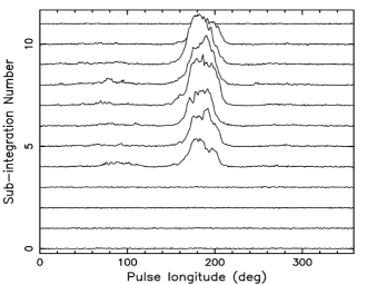
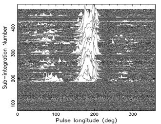
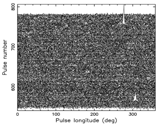
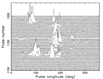
Figure 1: Top left: integrated pulse profiles formed from $\sim 63$ s sub-integrations (i.e. 250 pulses) for an $\sim 13$ min extract (i.e. 3000 pulses) from 121018$-$20cm. The sub-integration data is separated into consecutive profiles along the vertical axis (from bottom to top). The pulsar appears to only become active (and bright) in the fifth sub-integration. Top right: pulse stack of a slightly shorter data extract (pulses $450-2850$), plotted using sub-integration lengths of six pulses only ($\sim 1.5$ s). The greater time resolution afforded by these data display the short-time-scale modulation of the source which is not resolved when averaging over many pulses. Bottom left: single-pulse data for pulses $550-780$, showing two clearly detected weak-pulses during the otherwise apparent null phase. Bottom right: single-pulse data for pulses $1100-1200$, showing how the pulsar transitions between apparent null phases and the strong-mode of emission.

We find that this short-time-scale variability is inconsistent with interstellar scintillation, given the object’s narrow scintillation bandwidth ($\lesssim 40$ MHz) and relatively long scintillation time-scales at 1518 MHz ($\sim~{}5$ min, predicted by the NE2001 model; Cordes & Lazio 2002). As a result, we are confident that the emission modulation observed in this object is intrinsic.

3.2 Mode Description and Durations

Due to the pulse-to-pulse variability of the source, emission profiles formed from sub-integration data, i.e. the average of $\sim 10^{2-3}$ pulses, will not provide an accurate representation of the source’s emission characteristics or variability. Therefore, we used a boxcar algorithm with a variable width to locate single pulses with significant peaks, and facilitate correct characterization of the pulse properties attributed to each emission mode. Using our highest quality observations (see Table 2), we find that a $6\sigma$ sensitivity limit results in the most reliable location of discernible single-pulse emission. From those observations which were long enough to provide sufficient coverage of the source’s emission behaviour (i.e. the 20-cm data), we find that density of peak detections is directly related to the mode in which the pulsar assumes. Namely, during the weak mode of emission, peak detections arise sporadically between apparent null phases up to several hundred pulse periods. By contrast, peak detections are grouped in dense clusters of pulses with apparent nulls up to a few pulse periods only during the strong mode.

During the aptly named strong mode, we find that emission from the source is significantly enhanced, and hence more readily detectable, compared with that of the sporadically detected weak pulses. Furthermore, the pulsar exhibits a considerably broader main-pulse (MP) component in the average pulse profile than that in the weak mode. Interestingly, our data shows that strong-mode pulses are only emitted during relatively short burst periods ($\sim 60$ s up to $\sim 24$ min), with an average duration of approximately 500 s and a standard deviation of $\sim 400$ s (see Figs. 1 and $-$2). It is important to note, however, that 11 out of the 18 total detected bursts are not completely covered by our observations. Therefore, the quoted average duration for the emission bursts serves as a lower bound to the true value.

Upon closer inspection of the apparent null pulses, which are far more prevalent during the weak mode, we in fact find that the vast majority of them contain emission which is comparable to or below the detection thresholds of our data. This becomes clear upon averaging subsequent sequences of pulses ($\sim 10^{2}-10^{3}$ pulses), where low-level or underlying emission (UE) becomes more readily detectable with the number of pulses which are integrated over (see right panel of Fig. 2). Thus, we use the term apparent null to define pulses which are very weak and can be easily confused with null emission (c.f. Esamdin et al. 2005; Wang et al. 2007).

Due to the prevalence of apparent nulls in the pulsar, average profiles were formed in a few ways. That is, we formed average profiles with respect to the separate emission modes, and observing frequency, for all pulses and for only the $6\sigma$ detected pulses in the highest quality observations (see Table 2). For comparison, we also produced low-level emission profiles for the same observations, by locating and averaging pulses with no detectable peaks. From these data it is clear that while the average profiles of both the strong and weak modes exhibit emission both prior to and after the MP component $-$ which we refer to as precursor (PR) and postcursor (PC) emission components, respectively $-$ these components typically constitute a more significant proportion of the average emission profile during the weak mode, compared with that of the strong mode. We also find that the source does not exhibit a stable profile over the time-scales of our observations, in either the strong or weak modes of emission, regardless of the number of pulses integrated over (c.f. PSR B0656$+$14; Weltevrede et al. 2006). This is particularly evident during the strong mode of emission, which exhibits significant profile variations between successive observations.

Furthermore, we note that the pulses containing UE, during the apparent null state, are uniformly distributed throughout the data, which suggests that the pulsar may not truly undergo any conventional null phases (see e.g. Fig. 2). Rather, clearly detected weak pulses could represent those which are at the top end of the source’s pulse energy distribution (PED) during the otherwise apparent null mode. As such, we advance that the apparent null phases most likely do not represent a discrete emission state, and that they only constitute the lowest end of the PEDs of the strong and weak emission modes.

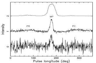
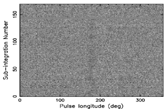
Figure 2: Left panel: from top to bottom, the average profiles formed from 121018$-$20 cm are shown for the strong and weak emission modes as well as for the UE during the apparent null phase. The on-pulse emission regions are also annotated. Each of the integrated profiles contains 1452, 70755 and 8360 pulses, respectively. Note that the pulse profiles are vertically offset from each other for clarity, and are normalized by their respective peak intensities. Right panel: grey-scale intensity map showing how the UE during the apparent null phase varies with time, after rebinning the data to 256 bins and integrating over consecutive groups of 500 pulses. Note that while the MP emission is clearly visible, the outer profile components are still below the noise threshold of the data.

In order to further constrain the pulse properties of the separate emission modes, we estimated the mean flux densities attributed to the pulsar, using the method outlined in Section 2, from the mode-separated average profiles. We also searched the high quality observations for the maximum peak-flux pulse densities to provide a direct brightness comparison with RRATs. Table 3 shows the results of this analysis.

Table 3: The observed emission properties of PSR J1107$-$5907. The columns are as follows: (1) type of emission from the pulsar (UE = underlying emission). (2) Centre frequency of the observation. (3) Equivalent pulse width of the brightest pulse which results in a boxcar with the same peak and integrated intensities as the observed pulse ($\omega=P\times\Sigma I/I_{\mathrm{peak}}$). (4) Peak flux density of the brightest pulse determined by using the single-pulse radiometer equation (see e.g. McLaughlin $\&$ Cordes 2003) and the receiver system specifications quoted (Manchester et al. 2013). (5) Peak pseudo-luminosity of the pulsar estimated by the equation $L_{\mathrm{peak}}=S_{\mathrm{peak}}\,d^{2}$ (Lorimer $\&$ Kramer 2005), where $d=1.28$ kpc is the distance to the source from the NE2001 model (Cordes $\&$ Lazio 2002). (6) Number of pulses used to compute the average emission properties. (7) Equivalent pulse width attributed to the average emission profile. (8) Mean flux density of the pulsar, calculated using the modified radiometer equation for the average profile (see e.g. Lorimer $\&$ Kramer 2005). (9) Number of pulses used to compute the average emission properties for the $6\sigma$ detected pulses. (10) Equivalent pulse width attributed to the average emission profile for the $6\sigma$ detected pulses. (11) Mean flux density of the pulsar, calculated using the modified radiometer equation for the average profile formed from the $6\sigma$ detected pulses.

Mode	$\nu$ (MHz)	$\omega$ (ms)	$\mathrm{S}_{\mathrm{peak}}$ (mJy)	$\mathrm{L}_{\mathrm{peak}}$ (Jy kpc2)	$N$	$\langle\omega\rangle$ (ms)	$\langle S\rangle$ (mJy)	$N_{6\sigma}$	$\langle\omega\rangle_{6\sigma}$ (ms)	$\langle S\rangle_{6\sigma}$ (mJy)
Strong	1369	1.00	9883	16.19	1676	24.67	11.05	919	24.68	14.65
Weak	1369	1.74	4178	6.85	130372	10.06	0.063	4056	10.05	0.55
UE	1369	$-$	$-$	$-$	15835	9.33	0.025	$-$	$-$	$-$
Weak	732	4.64	5638	9.24	35122	10.19	0.090	526	11.39	0.88
UE	732	$-$	$-$	$-$	4532	4.40	0.078	$-$	$-$	$-$
Weak	3094	1.54	2183	3.58	39834	11.17	0.039	1206	11.90	0.25
UE	3094	$-$	$-$	$-$	4068	4.50	0.014	$-$	$-$	$-$

We note that the peak flux densities of the brightest pulses detected during the strong and weak emission states are quite comparable at 20-cm. This is, however, in contrast to the large (a factor of $\sim 175$) difference in the flux densities of the mode-separated profiles, which implies that particularly energetic weak-mode pulses are exceptionally rare (c.f. the strong to UE flux density ratio of $\sim 440$:1). This is indeed observed in the data, given the large difference between the average flux densities of all mode-separated pulses and those attributed to the $6\sigma$ detected mode-separated pulses only. Moreover, we find that weak-mode pulses with flux densities $\geq 1$ Jy only constitute $\sim 0.03$ per cent of the pulses in the 20-cm band (c.f. $\sim 16$ per cent for the strong mode).

3.3 Pulse-energy Distributions

Given the remarkable variability of the source, we sought to further characterize its intensity fluctuations and apparent nulling behaviour through computing pulse-energy distributions (PEDs; see Weltevrede et al. 2006 for details on the method used) for the mode-separated observations in Table 2. For this analysis, PEDs were formed for the PR, MP and PC regions separately, as well as for the off-pulse (OP) region and the whole on-pulse regions for each observation. Due to the difference in the number of pulse longitude bins used, the OP energies were scaled such that they reflect the predicted noise fluctuations in the on-pulse regions. We note that no correction for interstellar scintillation was carried out as the dominant intensity fluctuations are caused by apparent nulling and mode-changing. Example results from this analysis are shown in Fig. 3, for the PEDs formed from the MP region.

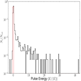
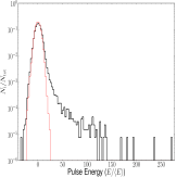
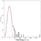
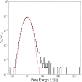
Figure 3: Integrated PEDs for the strong- and weak-mode pulses from the 20-cm data (top, left to right panels, respectively), as well as those for the 10-cm and 50-cm weak-mode pulses (bottom, left to right panels respectively). The PEDs are normalized by the average pulse energy $\langle E\rangle$ of each mode. The MP and OP energies are denoted by the thick black and thin red lines, respectively. The OP energies are scaled according to the proportion of MP to OP longitude bins used.

For the majority of our data, we find that the PEDs of the PR, PC and whole on-pulse regions typically do not have as clearly pronounced emission tails as those of the MP PEDs. This is particularly clear in the strong emission state, where the MP PED displays a narrower peak at zero PE and a more distinct emission tail towards large PEs compared with the other PEDs. This is in contrast to the results obtained in the 50-cm band, where the whole on-pulse PED shows greater evidence for emission compared with PEDs formed from PEs in the other profile regions. This disparity in the dominant PEDs can be explained by the frequency-dependent prevalence of bright emission in the respective emission windows (see $\S$ 3.3.2).

Overall, we do not find any conclusive evidence for nulls in the PEDs of either the strong or weak emission modes. That is, the PEDs formed from our data do not exhibit discernible breaks representative of a null distribution or divergence from a single distribution function. Rather, they appear to be continuous which is consistent with the hypothesis that the pulsar typically emits pulses under a relatively low PE regime, with some sporadic energetic emission that represents the top-end of its PED (particularly in the strong emission mode).

3.3.1 Pulse-energy Distribution Fitting

Typically, the PEDs of pulsars can be represented by single-component distributions (see e.g. Argyle & Gower 1972; Cairns 2004). However, in the presence of nulls, a given PED should either be bimodal or exhibit evidence for a functional transition. Such features in a PED can exist below the noise level. Therefore, we sought to confirm the results of the above analysis by fitting either a power-law or log-normal trial distribution to the mode-separated PEDs, in combination with a distribution of apparent nulls below the noise level, following the method described in Weltevrede et al. (2006). The functional forms of the fitted distributions are:

$$P_{\mathrm{pow}}(E) \propto E^{\,p}\,,$$ (1)

$$P_{\mathrm{logn}}(E) = \frac{\langle E\rangle}{\sqrt{2\pi}\sigma E}\exp\left[-\left(\ln\frac{E}{\langle E\rangle}-\mu\right)^{2}/\left(2\sigma^{2}\right)\right].$$ (2)

Since the power-law distribution extends to infinity, we incorporated a minimum pulse energy cut-off $E_{\mathrm{min}}$ into the power-law fit. Therefore, there are two fit parameters for both model distributions; i.e. $p$ and $E_{\mathrm{min}}$ for the power-law distribution and $\mu$ and $\sigma$ for the lognormal model distribution.

The effect of noise was accounted for by convolving the noise signature with the model PED for each observation. We estimated the noise signature by producing a symmetric distribution from the negative on-pulse energies. This ‘mirrored’ distribution is probably an oversimplification of the true noise variation, but provides a more realistic representation of the noise signature compared to the distribution derived from the very narrow OP region.

The requirement to include very low-level emission (apparent nulls) in a fit was also tested by optionally adding pulses with zero energy to a model distribution (before convolving this distribution with that of the noise), until the average energy $\langle E\rangle$ matched the observed value for a given set of fit parameters. The optimization was performed by minimizing the $\chi^{2}$ between the model and observed distributions (see Weltevrede et al. 2006 for details). Error bars on the fit parameters were also determined by finding the possible range of fit parameters which could still result in acceptable fits; i.e., with a significance probability above $5$ per cent. Table 4 shows the result of this analysis.

Table 4: The best-fit parameters of the model distributions. The reference key of each observation is denoted by REF and the type of pulses included in each fit is represented by ‘mode’. The power-law exponent and energy cut-off are represented by $p$ and $E_{\mathrm{min}}$, while the log-normal mean and standard deviation are given by $\mu$ and $\sigma$ respectively. The apparent NF, total $\chi^{2}$, number of degrees of freedom $N_{\mathrm{d.o.f.}}$ and significance probability $P(\chi^{2})$ are also tabulated.

REF	Mode	$p$	$E_{\mathrm{min}}$	$\mu$	$\sigma$	NF (per cent)	$\chi^{2}$	$N_{\mathrm{d.o.f.}}$	$P(\chi^{2}\mathrm{,}$ per cent)
121018$-$20cm	Strong	$-1.29^{+0.03}_{-0.02}$	$400^{+300}_{-100}$	$-$	$-$	$48^{+5}_{-4}$	10.5	9	30.2
121019$-$20cm	Stronga	$-$	$-$	$-$	$-$	$-$	$-$	$-$	$-$
121018$-$20cm	Weak	$-$	$-$	$5.8^{+0.1}_{-0.1}$	$0.9^{+0.1}_{-0.1}$	$91.5^{+0.5}_{-0.5}$	56.1	22	19.2
121019$-$20cm	Weak	$-$	$-$	$6.1^{+0.1}_{-0.1}$	$0.9^{+0.1}_{-0.1}$	$88.9^{+0.3}_{-0.3}$	21.5	14	29.7
121020$-$10cm	Weak	$-$	$-$	$7.7^{+0.1}_{-0.2}$	$0.7^{+0.1}_{-0.6}$	$89^{+1}_{-5}$	16.5	20	97.1
121020$-$50cm	Weak	$-$	$-$	$8.7^{+0.2}_{-0.3}$	$0.8^{+0.2}_{-0.5}$	$93^{+1}_{-4}$	32.2	24	61.7

^aInsufficient number of pulses to perform the analysis.

Overall, we find that the best fits are typically obtained for the MP PEDs during both the strong and weak emission modes (except for the 50-cm data where the whole on-pulse PEDs provide the best results). We also note that the strong-mode PEDs are best fit using a power-law distribution as opposed to a lognormal distribution for the weak mode PEDs. For both modes of emission, an additional, apparent null distribution is required to converge the fits. Therefore, a simple, single-component distribution of the chosen functional forms cannot be used to describe the PEDs of PSR J1107$-$5907. However, this does not necessarily provide evidence for the existence (or absence) of actual emission cessation in the source, as the PED fitting cannot distinguish between zero PEs and a PED of very weak UE. Therefore, we advance that the PEDs of the source cannot be purely described by lognormal/ power-law statistics, and that the UE may possess a different functional form whose transition is below the noise level.

3.3.2 Longitude-resolved Pulse-energy Distributions

While the analysis of the integrated on-pulse energies allows for the determination of the apparent NF and general pulse properties of the source, it does not provide a complete picture of the pulse intensity fluctuations attributed to the object. This is emphasized by the fact that pulsed emission from pulsars generally exhibits variability as a function of pulse longitude. Therefore, we sought to characterize such intensity fluctuations, and determine the dominant emission regions, through computing longitude-resolved PEDs for the highest quality observations (refer to Table 2). Here, we separated pulse profiles out into four pulse longitude regions $-$ the OP, MP and most energetic portions of the PR and PC emission windows $-$ and accumulated individual pulse-longitude bin samples over these regions into separate PEDs, respectively. Fig. 4 shows the longitude-resolved PEDs which result from this analysis, along with the corresponding average profiles for the mode-separated observations chosen.

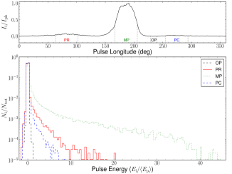
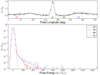
Figure 4: Longitude-resolved PEDs for the emission-mode separated observations. The plots show the results for the strong- and weak-mode pulses taken from the combined 20-cm data set (top and bottom panels, respectively). The top panel for each of these plots shows the average profile, normalized by the peak pulse intensity $I_{\mathrm{pk}}$ for each observation, with the emission regions annotated. The pulse energies are normalized by the average peak-energy $\langle E_{\mathrm{p}}\rangle$.

This analysis clearly confirms the prominence of emission in the MP and PR regions during the strong mode, where we observe a much greater number of high PE samples compared with that in the PC region. By comparison, emission in the weak mode is preferentially located to the PC and MP regions. In fact, we see that the pulsar emits an increasingly higher fraction of high-energy samples in the PC region during the weak emission mode towards lower frequencies. With the above in mind, it is clear that the pulse energy characteristics of the strong and weak modes are quite different which, subsequently, provides further evidence for a separation in the pulse populations.

3.3.3 Intensity-dependent Profile Variations

In several objects it has been shown that pulse profile variations can occur as a function of pulse intensity (see e.g. Gangadhara & Gupta 2001; Esamdin et al. 2005; Weltevrede et al. 2006). Motivated by this possibility, we formed integrated PE-separated profiles from the highest quality observations, for increasing average on-pulse intensities. We averaged $6\sigma$ detected pulses within energy ranges $E>5\,\langle E\rangle$, $3-5\,\langle E\rangle$, $1.5-3\,\langle E\rangle$ and $0-1.5\,\langle E\rangle$ (where $\langle E\rangle$ is the average pulse energy, over the whole on-pulse region, for a given observation), as shown in Fig. 5. The $6\sigma$ limit was chosen to mitigate the effect of apparent nulls on the average pulse energies and, subsequently, allow for the correct separation of pulses based on their integrated energies.

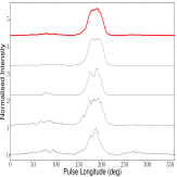
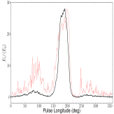
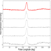
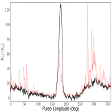
Figure 5: Pulse intensity fluctuation with respect to pulse longitude for the strong- (top panels) and weak-mode (bottom panels) pulses which exhibit $\geq 6\sigma$ peak detections. Left: the top thick line represents the average pulse profile, with successive lines (from top to bottom) denoting average profiles for pulses with $E>5\,\langle E\rangle$, $3-5\,\langle E\rangle$, $1.5-3\,\langle E\rangle$ and $0-1.5\,\langle E\rangle$, and for the strong mode contain 66, 34, 70 and 716 pulses, respectively. For the weak mode, these profiles contain 54, 157, 753 and 2472 averaged pulses, respectively. Note that all the profiles are normalized by their peak intensity and are offset for clarity. Right: scaled average profile (thick black line) and the brightest time sample for each pulse longitude bin (thin red line), compared with the average peak-energy of the profile $\langle E_{\mathrm{p}}\rangle$ (at a pulse longitude of $\sim 180\degr$).

In the strong-mode, we can clearly see that the average emission profile becomes increasingly dominated by the MP component with increasing average pulse intensity. By comparison, the weak-mode emission profiles become increasingly more dominated by the PR and PC components with increasing average intensity. This is also observed in both the 10- and 50-cm observing bands. While the PC component is very prominent in the highest energy band, and can often dominate over the MP, we note that the PE-separated plot for the weak-mode does not reflect the typical properties of the source. That is, we do not consider the average profile of the highest, weak-mode energy band to be close to a stabilized profile. This is because there is only a low number of pulses available for this analysis, coupled with the fact that only $\sim 60$ per cent of the highest energy band pulses display emission in the PC region. As such, we would expect the average PC component of the highest, weak-mode energy band to be up to just over half the relative strength of the average MP component, given a more stabilized profile through longer pulse integration.

Using only the $6\sigma$ pulse detections for the mode-separated observations again, we also determined the brightest pulse-energy sample for each pulse longitude bin, with respect to the average peak-energy of the respective profiles (see right panels of Fig. 5). In the strong mode of emission, we find that the brightest samples are preferentially distributed among the MP and PR pulse-longitude regions. By comparison, we note that the weak-mode emission is slightly more constrained. That is, the brightest pulse-energy samples are preferentially distributed over a smaller proportion of the separate emission regions during this emission mode, with the PC and MP components dominating. Overall, it is clear that the pulsar emits across almost the entire pulse longitude range.

3.4 Fluctuation Spectra

While the source is highly variable, there does not appear to be any regular periodicity in its intensity modulation. To test this hypothesis, we computed longitude-resolved fluctuation spectra (LRFS; Backer 1970), as well as two-dimensional fluctuation spectra (2DFS; Edwards & Stappers 2002) for several of the strong- and weak-mode single-pulse observations. We calculated the LRFS by taking Discrete Fourier Transforms (DFTs) along lines of constant pulse longitude in the pulse stacks, over successive blocks of 256 pulses. The resultant spectra were then averaged to provide a representation of the typical modulation properties of the data, and have pulse longitude on the horizontal axis and $P/P_{3}$ on the vertical axis (where $P_{3}$ is the subpulse repetition period; see bottom panels of Fig. 6).

We also computed the longitude-resolved variance ($\sigma_{i}^{2}$) and modulation index ($m_{i}=\sigma_{i}/\mu_{i}$) profiles (see top panels of Fig. 6) for the observations through vertical integration of the LRFS ($\mu_{i}$ is the average intensity at a given pulse longitude; see also Weltevrede et al. 2006 for more details). These parameters, in combination with the LRFS, were used to infer the presence of any intensity modulation and to determine whether it is random or periodic. To differentiate between an intensity or phase modulation, DFTs were also performed on separate pulse longitude regions within the LRFS to provide the 2DFS. The pulse longitude range was again separated into three on-pulse regions, i.e. the PR, MP and PC emission regions.

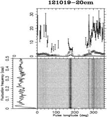
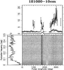
Figure 6: The modulation properties of PSR J1107$-$5907, observed during the strong mode of 121018$-$20cm and the weak modes of 121019$-$20cm and 121020$-$10cm (left to right respectively). The integrated pulse profile (solid line), longitude-resolved modulation index profile (solid line with error bars) and longitude-resolved standard deviation profile (open circles) are shown for each observation in the top panels. The bottom panels display the respective LRFS, with pulse longitude in degrees displayed on the horizontal axis. The side panels show the horizontal integration of the LRFS data, which represents the subpulse intensity modulation ($P/P_{3}$) of the pulse sequences.

For both modes of emission, we find that the most prominent intensity variation (i.e. highest modulation index) is typically associated with the PR and PC emission components, where the emission is more sporadic. Appreciable intensity modulation, similar to that seen in known pulsars, is also observed across the shoulders of the MP component. This is shown by the distinctive U-shapes in the modulation index profiles, which indicate that the dominant intensity modulation in the MP component is located away from its central peak (see also Weltevrede et al. 2006). Note that the 50-cm data were too weak to perform this analysis and were therefore excluded.

In the weak mode, the only significant LRFS feature can be observed in the lowest frequency bin ($P_{3}\geq 256~{}P$). However, we attribute this feature to the baseline correction method used, given that the use of different running mean lengths in the baseline normalization does not preserve this spectral feature. In the strong mode, a couple of spectral features dominate over the noise. The most significant of these is present at $P_{3}=9.6\pm 0.1~{}P$. Further investigation shows that this is a spurious signal which is only present in one of the 256 pulse-long blocks of data. Therefore, we conclude that the source only displays longitude-stationary non-periodic modulation.

3.5 Polarization Properties

In a number of pulsars, emission moding and/or transient emission behaviour is accompanied with changes in the source’s polarization properties, such as the presence of one or more orthogonal polarization modes (OPMs; see e.g. Gil et al. 1992; Karastergiou et al. 2011; Keith et al. 2013). With the above in mind, we sought to characterize the polarization properties of the separate emission states of PSR J1107$-$5907, so that we might elucidate the emission variability of the source. The results of this analysis are discussed below.

3.5.1 Rotation Measure Considerations

The rotation measure (RM) of a source is the term used to quantify the degree of Faraday rotation that its emission undergoes as it traverses through the interstellar medium (ISM; e.g. Wang et al. 2011 and references therein). Faraday rotation, and hence the RM, can be quantified by measuring the change in polarization position angle (PA) across a frequency band (e.g. Noutsos et al. 2008):

$$\Delta\mathrm{PA}=\frac{\mathrm{RM}\,c^{2}}{\nu^{2}}\,,$$ (3)

where $c$ is the speed of light and $\nu$ is the frequency of the electromagnetic waves. Following Noutsos et al. (2008), we measured the RM of PSR J1107$-$5907 in our polarization-calibrated observations using the RMFIT package, which they developed as part of the PSRCHIVE software suite (Hotan et al., 2004). This package, which uses a Bayesian likelihood test to find the best fitting RM to equation. (3), obtains an $\mathrm{RM}=23\pm 3$ rad m^-2 for our combined, time-integrated data. We note that this fit result serves as the first published measurement of the RM of PSR J1107$-$5907.

3.5.2 Polarization Fluctuations

PSR J1107$-$5907 exhibits very different polarization features during its separate emission modes (see Fig. 7). That is, the strong-mode emission features greater complexity, primarily in the MP component, and is more highly polarized than that of the weak mode on average. In order to ascertain whether there are any other polarization variations between the two modes, we analysed the polarization calibrated single-pulse data, which are capable of resolving short-time-scale fluctuations such as OPMs.

We measured the Stokes ($I$,$Q$,$U$,$V$) parameters and degree of linear ($L/I=\sqrt{Q^{2}+U^{2}}/I$; Backer & Rankin 1980) and circular ($V/I$) polarization for each pulse in our 20-cm data set. The PAs for these data were also measured, so as to properly characterize the polarization properties of the source. Given that random noise fluctuations can affect the reliability of data samples, we only used pulses which contained $6\sigma$ detections. We also restricted data samples to those with sufficient total intensities, i.e. $\mathrm{SNR}(I)\geq 3$, and required that the linear polarization components have SNR values above a threshold of two for both modes of emission. These thresholds act to reduce the total number of data points available for further analysis. However, they also act to significantly reduce noise contamination in the distributions of $L/I$, $V/I$ and PAs, which enable the recovery of the general polarization properties of the source, and facilitate further analysis of the data. Example polarization distributions from this analysis are shown in Fig. 7.

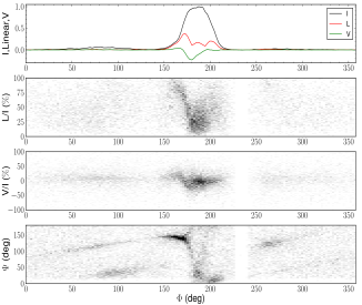
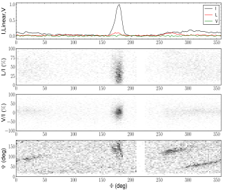
Figure 7: The single-pulse polarization properties of PSR J1107$-$5907 in 121018$-$20cm during its strong mode (left plot) and its weak mode in 121019$-$20cm (right plot) respectively. For each of the plots, the average emission profile is displayed in the top panel. Single-pulse distributions of $L/I$, $V/I$ and PA with respect to pulse longitude are also shown (from top to bottom respectively). Note the clear presence of the competing OPMs in the PR and PC regions for the strong and weak emission modes, respectively. The light vertical bands observed at fixed longitude throughout the data are an artefact of the baseline correction.

From this analysis, we find that the pulsar emits radiation from at least two competing polarization modes in both the strong and weak emission states. During the strong emission state, these competing modes are shown in the PR and PC regions. This is in contrast to the weak mode, where we only observe two competing polarization modes in the PC region. Interestingly, we also note the presence of non-OPM-like variations in PA in the central region of the MP component (at $\phi\sim$$$ and $\sim$$$) during the strong emission mode (c.f. PSR B0329$+$54; Edwards & Stappers 2004). Overall, we see that these variations are observed during the same observing runs and are only found to coincide with the emission mode changes in the source.

Considering the above variations in PA, it is clear that the polarization properties of the strong- and weak-mode pulses are quite different. Furthermore, we note that the average polarization properties of these pulses are dependent on the ratio of occurrence of the dominant OPMs (see Fig. 8). This is supported by the analysis of the strong-mode data from 121019$-$20cm, where only one competing PA-mode is observed over the short sequence of pulses ($\sim 60$ s).

3.5.3 Rotating-vector Model Fits

The magnetic inclination angle $\alpha$ and impact parameter $\beta$, of the line of sight with the magnetic axis of a pulsar, can be used to define the region where the observed radio emission is radiated from its magnetosphere. As such, these parameters are central to the determination of the emission geometry of a source. They can be constrained through fitting a source’s PA variation, as a function of pulse longitude, via the rotating vector model (RVM; Radhakrishnan & Cooke 1969; Komesaroff 1970). This simple model takes advantage of the close relationship between the PA and orientation of a pulsar’s dipolar magnetic field, to relate the rate of change of PA to the emission geometry of a source (Komesaroff, 1970):

$$\tan(\Psi-\Psi_{0})=\frac{\sin(\phi-\phi_{0})\,\sin\alpha}{\sin\zeta\,\cos\alpha-\cos\zeta\,\cos(\phi-\phi_{0})}\,,$$ (4)

where $\Psi$ is the PA at a pulse longitude $\phi$ and $\zeta=\alpha+\beta$ is the inclination of the observer direction to the rotation axis ($\Psi_{0}$ refers to the PA at the longitude of the fiducial plane $\phi_{0}$). The variation (or swing) in the linear PA, as the emission beam crosses our line-of-sight (LOS), is normally expected to be monotonic and take the form of an S-shaped curve (Radhakrishnan & Cooke, 1969). However, non-RVM like features such as 90-degree jumps in PA (a.k.a. OPMs) can also be observed, as seen in Fig. 7 (see also, e.g., Stinebring et al. 1984; Lyne & Smith 1989). While these features increase the complexity of PA-swing fits, they are often consistent with the RVM (see e.g. Lyne et al. 1971; Manchester et al. 1975; Backer & Rankin 1980; Stinebring et al. 1984).

Here, we use a $\chi^{2}$ minimization fitting method, based on equation (4), to constrain the $\alpha$ and $\beta$ parameters for PSR J1107$-$5907 from our polarization-calibrated observations, by optimizing $\phi_{0}$ and $\Psi_{0}$. For this analysis, we separated the time-integrated observations by emission mode, after correcting for Faraday rotation, and searched a grid of 200 by 200 possible $\alpha-\beta$ combinations for each data set. In order to obtain the most significant results, we compromised between the data quality and the number of fit points by only considering strong- and weak-mode PA values above $2\sigma$ thresholds. We also do not include strong-mode PA values from the pulse-longitude range $\phi=$$-$$$ in the fits, due to the sharp decreases in linear polarization and associated non-RVM consistent variations in PA (see Fig. 7). The best results from this analysis are shown in Fig. 8.

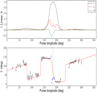
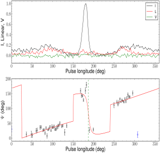
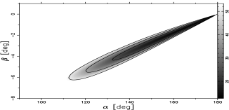
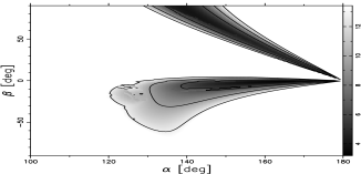
Figure 8: The best RVM fits to the integrated strong-mode data from 121018$-$20cm (left) and the integrated weak-mode data from 121019$-$20cm (right) respectively. Top panels: the average emission properties of the mode-separated observations, showing the total intensity profile, as well as the linear and circular polarization profiles. Middle panels: integrated PA data (crosses), with the best-fitting RVM (solid line) and location of the magnetic axis ($\phi_{0}$; dotted line) overlaid. PA data excluded from the fits are represented by the circles. Note the difference in location of the dominant PA distributions with respect to the separate modes of emission. Bottom panels: $\chi^{2}$-fit surfaces for the RVM fits, showing the $\alpha$ and $\beta$ fit constraints. The contours display the $\alpha-\beta$ combinations which result in reduced $\chi^{2}$ values of $1\sigma$, $2\sigma$ and $3\sigma$ within the nominal result.

We find that the PA-swing of the pulsar emission is best fit with the RVM using three orthogonal PA jumps (at $\phi=80\pm$$$, $135\pm$$$ and $235\pm$$$) for the strong mode and two orthogonal PA jumps (at $\phi=150\pm$$$ and $$$^{+10}_{-40}$) for the weak mode. Overall, we note that the PA swings of the strong and weak modes are largely consistent. The only noticeable difference between the two modes is the extra OPM during the strong mode, which diverges from the predictions of the RVM.

Unfortunately, the range of fit parameters provided by $3\sigma$ limits from the reduced $\chi^{2}$ plots does not result in very rigorous constraints. As such, we are only able to place conservative limits on the emission geometry of the source ($\alpha\gtrsim$$$ and $$$\lesssim\beta\lesssim$$$) from the mode-separated fits. We also performed this analysis for combined strong- and weak-mode data from 121018$-$20cm and 121019$-$20cm separately. The results of this analysis are consistent with the previous findings, but do not offer more stringent constraints on the emission geometry of the source.

We note that the PA is seen over a wide range of pulse longitude from the single pulses (refer to Fig. 7). However, we do not obtain better constraints on $\alpha$ and $\beta$ from the RVM fits if we include the most extreme PA values (e.g. from the $\Phi=$$-$$$ range). Rather, we obtain equivalent constraints to those obtained from the average profile PA curves (see Fig. 8).

Nevertheless, the above results are consistent with the source being a near-aligned rotator. This interpretation is further supported by the source’s extremely broad emission profile ($\sim$$$) and advanced age ($\tau\sim 447$ Myr), which are indications of magnetic alignment (see e.g. Rankin 1990; Tauris & Manchester 1998; Weltevrede & Johnston 2008; Young et al. 2010; Maciesiak et al. 2011).

4 Timing Analysis

In a substantial sample of pulsars, clear correlations can be seen between their pulse intensity/ shape and spin-down behaviour (see e.g. Kramer et al. 2006; Lyne et al. 2010; Keith et al. 2013). This leads us to suggest that similar changes might occur in PSR J1107$-$5907 if it is governed by the same magnetospheric process(es) (see e.g. Lyne et al. 2010; Li et al. 2012). To investigate such a relation between pulse intensity and rotational stability, we calculated timing residuals for PSR J1107$-$5907 using our entire data set (see e.g. Backer & Hellings 1986; Lorimer & Kramer 2005 for details on this method). As the observations displaying detectable emission contain a mixture of strong ($\sim 10$ per cent) and weak ($\sim 90$ per cent) emission profiles, times-of-arrival (TOAs) were calculated using two profile templates. These templates were formed from analytic fits to the highest SNR strong- and weak-mode profiles using PAAS, and were also aligned in time to remove any systematic offsets in measured TOAs. The latter process, along with the computation of the timing residuals (i.e. the difference between the observed and predicted TOAs) was carried out using the TEMPO2 package.

From this analysis, we find that the pulsar does not exhibit any significant timing noise; i.e. the resultant timing residuals for our data set are white (c.f. Hobbs et al. 2010). We also obtain an average $\dot{\nu}=-1.402\pm 0.001\times 10^{-16}$ s^-2, which is significantly lower than that of pulsars with detected spin-down variation ($\sim 10^{-15}$ to $10^{-13}$ s^-2; e.g. Lyne et al. 2010). This finding is consistent with the fits performed on the mode-separated TOAs, where we obtain spin parameters which are consistent within the uncertainties of the fitting procedure.

Following Young et al. (2012), we can approximate the minimum detectable spin-down rate variation in PSR J1107$-$5907 by

$$|\Delta\dot{\nu}_{\mathrm{av}}|\gtrsim\frac{3\times\Delta\nu_{\mathrm{mod}}}{T}\,,$$ (5)

where $|\Delta\dot{\nu}_{\mathrm{av}}|$ is the average change in $\dot{\nu}$ over the course of a period $T$, and $\Delta\nu_{\mathrm{mod}}$ is the precision of our timing model. Assuming an ideal scenario where the pulsar: (1) exhibits strong-mode bursts each of 24 min in length and a weak mode which lasts 6-hr; (2) is observed continuously over the course of two strong- and one weak-mode duration ($T\sim 22480$ s); (3) can be optimistically timed to an accuracy of $\sim 10^{-9}$ Hz, we would only expect to make a $3\sigma$ detection for $|\Delta\dot{\nu}_{\mathrm{av}}|/\dot{\nu}_{\mathrm{av}}\sim 950$. This limit is roughly 400 times greater than the largest spin-down variation currently seen in any pulsar (Camilo et al., 2012). Furthermore, as the object exhibits its weak emission mode for the majority of the time ($\sim 96$ per cent; see $\S$ 5.2), the average spin-down rate of the object will be largely determined by the $\dot{\nu}$ in this mode. As such, it is extremely unlikely that the source would be able to experience such a large variation in spin-down rate as the limit inferred above. With the above in mind, we surmise that a variable $\dot{\nu}$ will be exceedingly difficult to detect in PSR J1107$-$5907.

5 Discussion

5.1 Giant-like Pulses?

From the analysis of the pulse stacks and flux density measurements, it has been shown that PSR J1107$-$5907 can emit very energetic, sporadic emission in both its emission modes. The pulse energies of this particularly bright emission are observed to far exceed the energy threshold of $10~{}\langle E\rangle$, which is commonly used as an indication of giant pulse (GP) detections (e.g. Cairns et al. 2001). However, we find a number of dissimilarities between the bright emission of PSR J1107$-$5907 and classical GP emission. That is, we do not find evidence for a discernible break in the distribution of peak flux densities (see e.g. Argyle & Gower 1972; Lundgren et al. 1995; Karuppusamy et al. 2010). Nor do we observe any confinement in the pulse longitudes of the extremely bright pulses (see e.g. Knight et al. 2005). Moreover, these pulses also exhibit large pulse widths $\sim 1.6-27.0$ ms (c.f. approximately $0.4$ ns $-120~{}\mu$s for the Crab pulsar; Knight 2007; Hankins & Eilek 2007; Karuppusamy et al. 2010) and, hence, large duty cycles that are atypical of classical GPs ($10^{-2.2}\lesssim\delta\lesssim 10^{-1.0}$, c.f. $10^{-7.9}\lesssim\delta\lesssim 10^{-2.4}$ for the Crab; Karuppusamy et al. 2010).

As such, the brightest pulses attributed to PSR J1107$-$5907 cannot be considered classical GPs. Rather, we do find a strong relation with PSR B0656$+$14, which emits relatively wide pulses that can intermittently exceed well above the GP threshold $10~{}\langle E\rangle$ (up to $\sim 116~{}\langle E\rangle$ in fact; Weltevrede et al. 2006). As we will show in $\S$ 5.3 this suggests a connection with the RRAT population.

5.2 Detection Statistics

From the analysis of the longest observations, it is evident that the pulsar is active in its strong emission state for only a small percentage of time. During this mode, we see that the object preferentially emits bursts of pulses, with typical apparent nulls of up to a few pulse periods. The emission durations for the strong mode have been observed to be approximately $1-24$ min in length, and appear to have a uniform distribution, with an average duration $\langle T_{\mathrm{strong}}\rangle=500\pm 400$ s and highly variable apparent $\mathrm{NF}\sim 41-72$ per cent. However, given the small number of independent strong-mode detections (18), and number of observations which do not completely cover strong-mode bursts (10), it is difficult to accurately model these data.

Instead, we numerically estimated the best-fitting, average burst duration for the observed detection rates. Here, we assumed that the pulsar exhibits two, isolated strong-mode bursts over the course of a transit period at Parkes ($\sim 11$ h $27$ min), and that they appear uniformly distributed on a given day, in-line with the observed detections. This results in an estimated detection probability:

$$P_{\mathrm{strong}}=\frac{N_{\mathrm{strong}}}{N_{\mathrm{transit}}}\,,$$ (6)

where $N_{\mathrm{strong}}$ is the integer number of potential observations containing strong emission ($\langle T_{\mathrm{strong}}\rangle/T_{\mathrm{obs}}$), and $N_{\mathrm{transit}}$ is the integer number of observations spanning the entire transit period ($T_{\mathrm{transit}}/T_{\mathrm{obs}}$).

Using this method, we find that $\langle T_{\mathrm{strong}}\rangle=740\pm 20$ s results in the optimum number of strong-mode detections. This corresponds to a total, average emission duration of about 5900 pulses per Parkes transit period, and an inferred single-pulse detection rate of $g_{\mathrm{strong}}\sim 3.6$ per cent in the 20-cm band. Considering a typical observation length of $\sim 30$ min for a RRAT scan, we would then expect to obtain a strong-mode detection for every one in 12 observations in the 20-cm band. Further observation of the source at other frequencies is required before any statistics can be inferred at other observing wavelengths.

By contrast, detectable weak-mode pulses appear to be distributed uniformly throughout observations, between apparent nulls of typically up to several hundred pulse periods in length. As such, the UE during the apparent nulls in this source will not be revealed until sufficient pulse integration is performed. For our data, we obtain an increasing probability of weak-mode detection with $T_{\mathrm{obs}}$ until $\sim 80$ per cent and above rates are obtained for $T_{\mathrm{obs}}\gtrsim 60$ min. This result is consistent with the weak pulses assuming a log-normal intensity distribution (see $\S$ 3.3.1), with increasing number of pulses contributing to more significant detections. The low-level UE, or apparent null pulses, then represents those pulses which are not individually detected in our data due to intrinsic sensitivity thresholds (c.f. Esamdin et al. 2012 and references therein).

However, the above does not provide the complete picture for the weak-mode emission. If we only consider individually detectable weak-mode pulses (i.e. $\gtrsim 6\sigma$ detections), we obtain single-pulse detection rates of $g_{\mathrm{weak}}\sim 3$ per cent in the 10- and 20-cm bands, and $g_{\mathrm{weak}}\sim 1.5$ per cent in the 50-cm band from our data. This corresponds to detectable weak-mode pulses being emitted at a rate of approximately 1 weak pulse every 33 rotations, or $\sim 430$ h^-1 in the 10- and 20-cm bands, and 1 weak pulse roughly every 67 rotations, or $\sim 240$ h^-1 in the 50-cm band. Therefore, this pulsar could be confused as a RRAT-like source if it were only observed over short time-scales (see also $\S$ 5.3).

To further investigate the prospect of confusion between null emission and very weak emission in the pulsar population, we sought to characterize the number of sources which could be detected in a potential weak mode of emission. In this context, we assume that all pulsars exhibit a strong and weak mode of emission, with a flux density ratio of $S_{\mathrm{strong}}/S_{\mathrm{weak}}$. Given that the Parkes telescope has been the most successful pulsar survey instrument to date, we also assume that observations are coordinated over a range of pulse integration time-scales, with a telescope of the same size (i.e. 64 m), possessing system parameters typical of the Parkes Multibeam receiver (see Manchester & et al. 2013). Furthermore, we assume that this telescope can theoretically observe the entire known pulsar population, which have defined period, equivalent width and flux density parameters (refer to the ATNF catalogue; Manchester et al. 2005). From this analysis, we find that only a very small fraction of the pulsar population (up to $\sim 11$ per cent) could be detected by a 64-m telescope in a potential weak state, assuming a flux density ratio of $\sim 100$ between the strong and weak modes and an observation time of 30-min (see Fig 9). Note that the probability of detection becomes even lower for higher flux density ratios, assuming the same integration time.

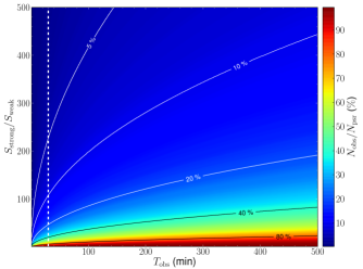
Figure 9: Parkes Multibeam detection statistics for pulsars in the ATNF catalogue, assuming a $5\sigma$ detection threshold for a potential weak emission mode. The dotted line overlaid traces the detection statistics for an observation time of 30 min. Note that only $\sim 11$ per cent of sources would potentially be detected in a weak emission state assuming a flux density ratio of 100 between the strong and weak modes for this integration time. It is clear that the majority of sources would only be detected in a particularly weak emission state after substantial pulse integration, which is atypical of current intermittent studies.

With the above in mind, it is clear that the detection statistics for many sources are intrinsically linked to the length of observing runs. This provides strong motivation for increasing the typical length of observations in sources which exhibit some form of moding behaviour and/or potential nulling. It also suggests that the interpretation of nulls as true emission cessation should coincide with the choice of observing system (e.g. observation length and telescope) used, as previously mentioned by several authors (see e.g. Keane et al. 2011; Burke-Spolaor & et al. 2011; Lyne 2013).

While there is yet no evidence for emission in the off-state of a substantial number of intermittent pulsars (e.g. Kramer et al. 2006; Camilo et al. 2012; Lorimer et al. 2012; Young et al. 2012; Gajjar et al. 2012), we suggest that the apparent null-states of many other known nulling sources should be studied for the existence of low-level emission, given that they may in fact undergo extreme mode changes without the need for the complete cessation of emission (c.f. Esamdin et al. 2005; Wang et al. 2007). We further advance that even the deep observations of several intermittent sources with existing telescopes (see e.g. Kramer et al. 2006; Lorimer et al. 2012) may not be sufficient to discover an extremely low level of emission. This indicates that future telescopes such as the SKA will be required to discern the true behaviour of moding and/or nulling objects.

5.3 A RRAT Connection?

PSR J1107$-$5907 shares a number of similarities with the RRAT population. As shown above, the source exhibits a low single-pulse detection rate, particularly in its weak emission state, which is consistent with the observed detection rates of RRATs. Furthermore, the object displays extreme brightness variations which are quantified by typical modulation indices that are comparable to, or exceed those of RRAT-like sources (refer to Table 5, see also Weltevrede et al. 2006; Serylak & et al. 2009; Weltevrede et al. 2011). The peak pseudo-luminosities of the pulsar, associated with the separate active emission modes, are also consistent with the average associated with currently known RRATs ($\langle L_{\mathrm{peak}}\rangle_{{}_{\mathrm{RRAT}}}=5\pm 8$ Jy kpc²; c.f. Table 3).

Table 5: The average modulation properties of PSR J1107$-$5907, with respect to emission region, for the observations chosen for spectra analysis.

REF	Mode	$\langle m_{\mathrm{PR}}\rangle$	$\langle m_{\mathrm{MP}}\rangle$	$\langle m_{\mathrm{PC}}\rangle$
121018$-$20cm	Strong	$9\pm 2$	$6\pm 2$	$8\pm 3$
121019$-$20cm	Stronga	$-$	$-$	$-$
121018$-$20cm	Weak	$11\pm 4$	$8\pm 2$	$15\pm 6$
121019$-$20cm	Weak	$16\pm 3$	$6\pm 2$	$16\pm 5$
121020$-$10cm	Weak	$7\pm 1$	$7\pm 2$	$10\pm 3$

^aInsufficient number of pulses to perform the analysis.

While the above similarities with conventional RRATs are interesting in their own right, it is perhaps more interesting to compare the pulsar with objects such as PSRs J0941$-$39 and B0826$-$34. These pulsars are currently the only sources to have been shown to exhibit ‘conventional’ nulling and RRAT-like behaviour (Burke-Spolaor & Bailes, 2010; Burke-Spolaor & et al., 2012; Esamdin et al., 2012). PSR J1107$-$5907 exhibits similar behaviour to these pulsars, apart from the fact that there is discernible emission present in its apparent nulls after sufficient pulse averaging ($\sim 10^{3}$ pulses). The requirement to average over pulses to detect this UE suggests that if the pulsar were placed farther away, then this source would appear more similar to such RRAT-like objects (see e.g. Weltevrede et al. 2006; Keane et al. 2010).

Indeed, when a factor of $\sim 16$ increase in Gaussian noise is introduced to the weak-mode pulses of PSR J1107$-$5907 (i.e. mimicking a factor of $\sim 4$ increase in Earth-pulsar distance), we find that the detection rates approach close to zero for integrated groups of consecutive pulses ($\sim 30$ min in duration, c.f. typical RRAT scans). Whereas, the single-pulse detection rate for the weak mode reduces to $\sim 65$ h^-1 in the 20-cm band, when introducing the same excess noise (see Fig. 10). This is in contrast to the strong mode of emission, where the pulsar is detected in both single pulses and in the average profiles, or not at all, depending on the level of additional noise introduced. Therefore, the strong-mode of PSR J1107$-$5907 would likely represent the ‘pulsar-like’ emission states of PSRs J0941$-$39 and B0826$-$34, and the weak mode would likely represent their RRAT-like modes if the object were placed at a farther distance.

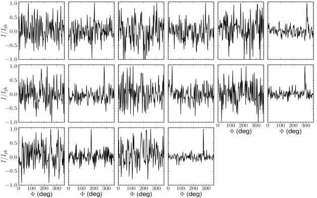
Figure 10: Simulated emission profiles for the weak-mode emission of 121019-20cm, which contain a factor of $\sim 16$ increase in Gaussian noise compared with the observed data. From left to right, alternately, are the average profiles for successive 30-min integrations and the brightest single-pulse profiles for the corresponding pulse ranges. Note that the pulsar is rarely detected in the average profiles, if at all, while single-pulse detections are observed in the majority of the panels.

These findings provide additional support to the idea that RRATs are not a distinct class of objects in the general pulsar population. Rather, they most likely consist of a mixed population of modulated pulsars with extended PEDs (Weltevrede et al., 2006) and extreme nulling pulsars (Burke-Spolaor & Bailes, 2010; Keane et al., 2010).

6 Conclusions

Our analysis of the emission behaviour of PSR J1107$-$5907 has shown that the source exhibits a very high degree of pulse-to-pulse variability, which is comparable to that observed in RRAT-like objects. Remarkably, it has also been shown that the flux density ratio of the average bright to weakest emission is of the order of $\sim 440:1$, which is considered to be a record in this work. These attributes have led previous authors to suggest the presence of a null mode of emission, in addition to the strong and weak modes observed in our data. However, we have discovered low-level emission during the apparent null phases of the longer weak modes, through integration of $\gtrsim 10^{2}$ pulses which exhibit no discernible peaks (see $\S$ 3.1). This emission resembles the weak-mode average profile and can, therefore, be considered to be representative of emission from the lowest end of the PED for the source. This indicates that the source most likely only exhibits two modes of emission, with UE being present, during both the strong and weak modes of emission. As such, we advance that the nulls observed in many intermittent objects may just represent a transition to a particularly weak mode, rather than the complete cessation of emission (see $\S$ 5.2).

We have also found that the source emits strong-mode pulses in isolated bursts of $\sim 200-6000$ pulses at a time, with the appearance of apparent nulls over time-scales of up to a few pulses in between detections. While no discernible emission was discovered through integration of these apparent nulls, we advance that such emission should be unveiled after a sufficient number of strong-mode pulses (i.e. $\gtrsim 10^{2}$ pulses) containing apparent nulls are integrated. We also infer a strong-mode detection probability of $\sim 8$ per cent for observation scans of 30-min in duration.

During the weak mode of emission, we find that the source exhibits detectable emission over time-scales of up to a few pulse periods at a time, with apparent nulls typically lasting up to several hundred pulse periods. The single-pulse detection probability for the source during this mode is found to be $\sim 3$ per cent in the 10- and 20-cm bands, and $\sim 1.5$ per cent in the 50-cm band. This corresponds to single-pulse detection rates of $\sim 430$ h^-1 for observing wavelengths of 10 and 20 cm, and $\sim 240$ h^-1 at 50 cm. We also find that $\gtrsim 1$ h integrations of weak-mode pulses typically result in detections. This emphasizes the need for long observing runs ($\gtrsim 1$ h) when observing moding and/or transient pulsars.

We also provide additional evidence for magnetic alignment in PSR J1107$-$5907. However, we stress that further polarization measurements of this source are required to support this finding and fully map the magnetospheric emission from the source.

Due to the low spin-down rate for this source, we did not detect a variable $\dot{\nu}$. This follows from the findings of Young et al. (2012), who advance that not all transient and/or moding objects will display detectable variations in $\dot{\nu}$. As such, we suspect that only instruments such as the SKA will be able to provide sufficient depth to the timing studies of such variable pulsars.

Furthermore, we find that the pulsar can be reconciled with objects such as PSRs J0941$-$39 and B0826$-$34 if it were placed at a farther distance. Coupled with the general similarities of the source with RRATs, this further indicates that RRATs are most likely not part of a distinct class of pulsars, as suggested by previous authors.

While it is not currently clear what the trigger mechanism for the behaviour observed in PSR J1107$-$5907 is, it is clear that future re-observation of this source should help shed light on its behaviour. In particular, high-energy studies of the source, during its strong mode, should prove beneficial to constraining a potential driving mechanism, given the various observationally verifiable predictions of each theory (see e.g. Hermsen & et al. 2013).

7 Acknowledgements

We are grateful to S. Oslowski, J. Sarkissian, J. Quick and D. Yardley for help in obtaining data which were used in this work. We would also like to thank the members of the Parkes P786 observing programme for contributing observations. Additional thanks go to R. M. Shannon and R. Warmbier for providing useful comments which have contributed to this research. NJY acknowledges support from the National Research Foundation.

References

- Argyle & Gower (1972) Argyle E., Gower J. F. R., 1972, ApJ, 175, L89
- Backer (1970) Backer D. C., 1970, 227, 692
- Backer & Hellings (1986) Backer D. C., Hellings R. W., 1986, Ann. Rev. Astr. Ap., 24, 537
- Backer & Rankin (1980) Backer D. C., Rankin J. M., 1980, ApJS, 42, 143
- Burke-Spolaor & Bailes (2010) Burke-Spolaor S., Bailes M., 2010, MNRAS, 402, 855
- Burke-Spolaor & et al. (2011) Burke-Spolaor S., et al. 2011, MNRAS, 416, 2465
- Burke-Spolaor & et al. (2012) Burke-Spolaor S., et al. 2012, MNRAS, 423, 1351
- Cairns (2004) Cairns I. H., 2004, ApJ, 610, 948
- Cairns et al. (2001) Cairns I. H., Johnston S., Das P., 2001, ApJ, 563, L65
- Camilo et al. (2012) Camilo F., Ransom S. M., Chatterjee S., Johnston S., Demorest P., 2012, ApJ, 746, 63
- Cordes & Lazio (2002) Cordes J. M., Lazio T. J. W., 2002, preprint (arXiv:astro-ph/0207156)
- Cordes & Shannon (2008) Cordes J. M., Shannon R. M., 2008, ApJ, 682, 1152
- Edwards & Stappers (2002) Edwards R. T., Stappers B. W., 2002, A&A, 393, 733
- Edwards & Stappers (2004) Edwards R. T., Stappers B. W., 2004, A&A, 421, 681
- Esamdin et al. (2012) Esamdin A., Abdurixit D., Manchester R. N., Niu H. B., 2012, ApJL, 759, L3
- Esamdin et al. (2005) Esamdin A., Lyne A. G., Graham-Smith F., Kramer M., Manchester R. N., Wu X., 2005, MNRAS, 356, 59
- Gajjar et al. (2012) Gajjar V., Joshi B. C., Kramer M., 2012, MNRAS, 424, 1197
- Gangadhara & Gupta (2001) Gangadhara R. T., Gupta Y., 2001, ApJ, 555, 31
- Geppert et al. (2003) Geppert U., Rheinhardt M., Gil J., 2003, A&A, 412, L33
- Gil et al. (1992) Gil J. A., Lyne A. G., Rankin J. M., Snakowski J. K., Stinebring D. R., 1992, A&A, 255, 181
- Hankins & Eilek (2007) Hankins T. H., Eilek J. A., 2007, ApJ, 670, 693
- Hermsen & et al. (2013) Hermsen W., et al. 2013, 339, 436
- Hobbs et al. (2010) Hobbs G., Lyne A. G., Kramer M., 2010, MNRAS, 402, 1027
- Hobbs et al. (2006) Hobbs G. B., Edwards R. T., Manchester R. N., 2006, MNRAS, 369, 655
- Hotan et al. (2004) Hotan A. W., van Straten W., Manchester R. N., 2004, PASA, 21, 302
- Kalapotharakos et al. (2012) Kalapotharakos C., Kazanas D., Harding A., Contopoulos I., 2012, ApJ, 749, 2
- Karastergiou et al. (2011) Karastergiou A., Roberts S. J., Johnston S., Lee H., Weltevrede P., Kramer M., 2011, MNRAS, 415, 251
- Karuppusamy et al. (2010) Karuppusamy R., Stappers B. W., van Straten W., 2010, A&A, 515, A36+
- Keane et al. (2011) Keane E. F., Kramer M., Lyne A. G., Stappers B. W., McLaughlin M. A., 2011, MNRAS, 415, 3065
- Keane et al. (2010) Keane E. F., Ludovici D. A., Eatough R. P., Kramer M., Lyne A. G., McLaughlin M. A., Stappers B. W., 2010, MNRAS, 401, 1057
- Keith et al. (2013) Keith M. J., Shannon R. M., Johnston S., 2013, MNRAS, 432, 3080
- Knight (2007) Knight H. S., 2007, MNRAS, 378, 723
- Knight et al. (2005) Knight H. S., Bailes M., Manchester R. N., Ord S. M., 2005, ApJ, 625, 951
- Komesaroff (1970) Komesaroff M. M., 1970, 225, 612
- Kramer et al. (2002) Kramer M., Johnston S., van Straten W., 2002, MNRAS, 334, 523
- Kramer et al. (2006) Kramer M., Lyne A. G., O’Brien J. T., Jordan C. A., Lorimer D. R., 2006, 312, 549
- Li et al. (2012) Li J., Spitkovsky A., Tchekhovskoy A., 2012, ApJL, 746, L24
- Lorimer & et al. (2006) Lorimer D. R., et al. 2006, MNRAS, 372, 777
- Lorimer & Kramer (2005) Lorimer D. R., Kramer M., 2005, Handbook of Pulsar Astronomy. Cambridge University Press, Cambridge
- Lorimer et al. (2012) Lorimer D. R., Lyne A. G., McLaughlin M. A., Kramer M., Pavlov G. G., Chang C., 2012, ApJ, 758, 141
- Lundgren et al. (1995) Lundgren S. C., Cordes J. M., Ulmer M., Matz S. M., Lomatch S., Foster R. S., Hankins T., 1995, ApJ, 453, 433
- Lyne (2013) Lyne A., 2013, in van Leeuwen J., ed., IAU Symp. Vol. 8 of Symp. S291 (Neutron Stars and Pulsars: Challenges and Opportunities after 80 years), Timing noise and the long-term stability of pulsar profiles. p. 183
- Lyne et al. (2010) Lyne A., Hobbs G., Kramer M., Stairs I., Stappers B., 2010, 329, 408
- Lyne & Smith (1989) Lyne A. G., Smith F. G., 1989, MNRAS, 237, 533
- Lyne et al. (1971) Lyne A. G., Smith F. G., Graham D. A., 1971, MNRAS, 153, 337
- Maciesiak et al. (2011) Maciesiak K., Gil J., Ribeiro V. A. R. M., 2011, MNRAS, 414, 1314
- Manchester & et al. (2013) Manchester R. N., et al. 2013, PASA, 30, 17
- Manchester et al. (2005) Manchester R. N., Hobbs G. B., Teoh A., Hobbs M., 2005, AJ, 129, 1993
- Manchester et al. (1975) Manchester R. N., Taylor J. H., Huguenin G. R., 1975, ApJ, 196, 83
- McLaughlin & Cordes (2003) McLaughlin M. A., Cordes J. M., 2003, ApJ, 596, 982
- McLaughlin & et al. (2006) McLaughlin M. A., et al. 2006, 439, 817
- Noutsos et al. (2008) Noutsos A., Johnston S., Kramer M., Karastergiou A., 2008, MNRAS, 386, 1881
- O’Brien (2010) O’Brien J., 2010, PhD thesis, The University of Manchester
- O’Brien et al. (2006) O’Brien J. T., Kramer M., Lyne A. G., Lorimer D. R., Jordan C. A., 2006, Chinese J. Astron. Astrophys. Suppl., 6, 020000
- Radhakrishnan & Cooke (1969) Radhakrishnan V., Cooke D. J., 1969, Astrophys. Lett., 3, 225
- Rankin (1990) Rankin J. M., 1990, ApJ, 352, 247
- Ribeiro (2008) Ribeiro V. A. R. M., 2008, PhD thesis, The University of Manchester
- Serylak & et al. (2009) Serylak M., et al. 2009, MNRAS, 394, 295
- Stinebring et al. (1984) Stinebring D. R., Cordes J. M., Rankin J. M., Weisberg J. M., Boriakoff V., 1984, ApJS, 55, 247
- Tauris & Manchester (1998) Tauris T. M., Manchester R. N., 1998, MNRAS, 298, 625
- Timokhin (2010) Timokhin A. N., 2010, MNRAS, 408, L41
- Urpin & Gil (2004) Urpin V., Gil J., 2004, A&A, 415, 305
- Wang et al. (2011) Wang C., Han J. L., Lai D., 2011, MNRAS, 417, 1183
- Wang et al. (2007) Wang N., Manchester R. N., Johnston S., 2007, MNRAS, 377, 1383
- Weltevrede et al. (2006) Weltevrede P., Edwards R. T., Stappers B. W., 2006, A&A, 445, 243
- Weltevrede & Johnston (2008) Weltevrede P., Johnston S., 2008, MNRAS, 387, 1755
- Weltevrede et al. (2011) Weltevrede P., Johnston S., Espinoza C. M., 2011, MNRAS, 411, 1917
- Weltevrede et al. (2006) Weltevrede P., Stappers B. W., Rankin J. M., Wright G. A. E., 2006, ApJ, 645, L149
- Weltevrede et al. (2006) Weltevrede P., Wright G. A. E., Stappers B. W., Rankin J. M., 2006, A&A, 458, 269
- Young et al. (2010) Young M. D. T., Chan L. S., Burman R. R., Blair D. G., 2010, MNRAS, 402, 1317
- Young et al. (2013) Young N. J., Stappers B. W., Lyne A. G., Weltevrede P., Kramer M., Cognard I., 2013, MNRAS, 429, 2569
- Young et al. (2012) Young N. J., Stappers B. W., Weltevrede P., Lyne A. G., Kramer M., 2012, MNRAS, 427, 114
- Zhang et al. (2007) Zhang B., Gil J., Dyks J., 2007, MNRAS, 374, 1103
- Zhang et al. (1997) Zhang B., Qiao G. J., Lin W. P., Han J. L., 1997, ApJ, 478, 313