Measurement of the $\eta\to\pi^{+}\pi^{-}\pi^{0}$ Dalitz plot distribution

Abstract

Dalitz plot distribution of the $\eta\to\pi^{+}\pi^{-}\pi^{0}$ decay is determined using a data sample of $1.2\cdot 10^{7}$ $\eta$ mesons from $pd\to^{3}\textrm{He}\eta$ reaction at 1 GeV collected by the WASA detector at COSY.

I Introduction

The amplitude of the isospin violating decays $\eta\to\pi^{+}\pi^{-}\pi^{0}$ and $\eta\to\pi^{0}\pi^{0}\pi^{0}$ is dominated by a term proportional to the light quark mass difference $(m_{d}-m_{u})$ since the electromagnetic contribution is suppressed Sutherland (1966); Baur et al. (1996); Ditsche et al. (2009). This makes the decays a sensitive probe of the light quark masses Leutwyler (1996). The leading term for the partial decay widths of the two decay modes is proportional to $Q^{-4}$ where $Q^{2}$ is defined as the following combination of the light quark masses Kaplan and Manohar (1986):

$$Q^{2}=\frac{m_{s}^{2}-\hat{m}^{2}}{m_{d}^{2}-m_{u}^{2}},\ \ \hat{m}=\frac{1}{2}(m_{u}+m_{d}).$$ (1)

The determination of the $Q$ parameter requires knowledge of the experimental value of at least one of the $\eta\to\pi^{+}\pi^{-}\pi^{0}$, $\eta\to\pi^{0}\pi^{0}\pi^{0}$ partial decay widths and the corresponding proportionality factors.

Experimental determination of the partial decay widths requires knowledge of the $\eta$ radiative width, $\Gamma_{\gamma\gamma}$, and the relative branching ratios $BR(\eta\to\pi^{0}\pi^{0}\pi^{0})/BR(\eta\to\gamma\gamma)$ and $BR(\eta\to\pi^{+}\pi^{-}\pi^{0})/BR(\eta\to\gamma\gamma)$. The radiative width could be determined by measuring cross section of the $\eta$ meson two photon production using e.g. Primakov effect or $e^{\pm}e^{-}\to e^{\pm}e^{-}\eta$ process. The knowledge of the Dalitz plot distributions for the $\eta\to 3\pi$ decays will in principle contribute to all measurements involving these final states. For example $\Gamma_{\gamma\gamma}$ was recently extracted from the cross section of the two photon production $e^{+}e^{-}\to e^{+}e^{-}\eta$ where the $\eta$ meson was tagged by the $\eta\to\pi^{0}\pi^{0}\pi^{0}$ and $\eta\to\pi^{+}\pi^{-}\pi^{0}$ decay modes Babusci et al. (2013a).

The calculations of the proportionality factors could be carried out in the low energy effective field theory of the strong interactions, Chiral Perturbation Theory (ChPT). The process was calculated up to next-to-next-leading order (NNLO) Bell and Sutherland (1968); Cronin (1967); Gasser and Leutwyler (1985); Bijnens and Ghorbani (2007). The ChPT leading order (LO) result together with the measured value of the $\eta\to\pi^{+}\pi^{-}\pi^{0}$ decay width of $300\pm 12$ eV Beringer et al. (2012) leads to $Q$ equal 15.6 (Tab. 1). The next-to-leading order (NLO) gives the $Q$ value 28% larger where half of the increase comes from $\pi\pi$ re-scattering between final state pions Roiesnel and Truong (1981); Gasser and Leutwyler (1985). Finally the NNLO order increases the value by an additional 14%. The values of $Q$ extracted from various analyses are summarized in Tab. 1.

Calculations:	Q
LO Bijnens and Ghorbani (2007)	15.6
NLO Bijnens and Ghorbani (2007)	20.1
NNLO Bijnens and Ghorbani (2007)	22.9
dispersive Anisovich and Leutwyler (1996)	$22.7(8)$
dispersive Kambor et al. (1996)	$22.4(9)$
dispersive (PLM) Kampf et al. (2011)	$23.1(7)$
Lattice QCD av. Aoki et al. (2013)	$22.6(7)(6)$

Table 1: Values of $Q$ obtained from the $\eta\rightarrow 3\pi$ decay. In addition a lattice QCD estimate is shown for comparison.

The reliability of the calculations leading to the proportionality factor could be tested by comparing the experimental and theoretical Dalitz plots for both the neutral and charged modes. Such comparison constitutes a sensitive test of the convergence of the SU(3) ChPT expansion. For the neutral decay mode, where the Dalitz plot density is described by a single parameter up to quadratic terms, the experiments provide a consistent, precise value Alde et al. (1984); Abele et al. (1998a); Achasov et al. (2001); Tippens et al. (2001); Bashkanov et al. (2007); Adolph et al. (2009); Prakhov et al. (2009); Unverzagt et al. (2009); Ambrosino et al. (2010). However, reproduction of this value has turned out to be a challenge for the ChPT calculations. For the $\eta\to\pi^{+}\pi^{-}\pi^{0}$ decay mode, where the are more parameters to describe Dalitz plot density, there is basically only one modern, high statistics experiment Ambrosino et al. (2008).

The amplitudes for the $\eta\to 3\pi$ decays could be also determined using unitarity and analyticity and the $\pi\pi$ phase shifts up to some subtraction constants. These subtraction constants can be determined by matching to the results of the ChPT calculations Kambor et al. (1996); Anisovich and Leutwyler (1996) and thus improving convergence of the ChPT expansion. Alternatively the subtraction constants can be obtained directly from fits to the experimental Dalitz plot distributions using only the most reliable constraints from ChPT. In recent years two such data driven dispersive approaches have emerged: from Bern-Lund-Valencia (BLV) group Colangelo et al. (2009) and from Prague-Lund-Marseille (PLM) group Kampf et al. (2011). Both approaches rely in large extent on the experimental Dalitz plot data from and promise a precise determination of $Q$.

Another aspects of the $\eta\to 3\pi$ decay such as isospin violation effects in low-energy $\pi\pi$ scattering are addressed by Non-Relativistic Effective Field Theory (NREFT), developed first for low-energy $\pi\pi$ scattering and decay $K\rightarrow 3\pi$ Colangelo et al. (2006) decays and subsequently was applied to $\eta\rightarrow 3\pi$ decays Gullstrom et al. (2009); Schneider et al. (2011). A more model dependent analysis providing uniform treatment of all three pseudoscalar $\eta$ and $\eta^{\prime}$ decay modes, including $\eta\rightarrow 3\pi$ was pursued in Ref. Borasoy and Nissler (2005).

The Dalitz plot for $\eta\to\pi^{+}\pi^{-}\pi^{0}$ is expressed using normalized variables $X$ and $Y$:

$$X=\sqrt{3}\frac{T_{+}-T_{-}}{Q_{\eta}};\ \ \ Y=\frac{3T_{0}}{Q_{\eta}}-1,$$ (2)

where $T_{+}$, $T_{-}$, $T_{0}$ are kinetic energies of the charged and neutral pions in the $\eta$ meson rest frame. $Q_{\eta}$ is the excess energy for the decay:

$$Q_{\eta}=T_{+}+T_{-}+T_{0}$$ (3)

or equivalently $Q_{\eta}=m_{\eta}-2m_{\pm}-m_{0}$ where $m_{\pm}$ and $m_{0}$ are the masses of the charged and neutral pions. A polynomial parametrization is often used to represent the squared amplitude for the decay:

$$|\mathcal{A}(X,Y)|^{2}\propto\rho(X,Y)=N\left(1+aY+bY^{2}+cX+dX^{2}+eXY+fY^{3}+gX^{2}Y+hX^{3}\right),$$ (4)

where $\rho(X,Y)$ is the Dalitz plot density, $N$ is a normalization factor and $a,b,...,g,h$ are Dalitz plot parameters. The terms with odd powers of the $X$ variable, like $c$, $e$ and $h$, should be zero as they imply charge conjugation violation in strong or electromagnetic interactions. The Dalitz plot parameters from various theoretical predictions and from experiments are given in Tab. 2.

Calculations	$-a$	b	d	f	g
LO Bijnens and Ghorbani (2007)	$1.039$	$0.27$	$0.000$	0.000	$-$
NLO Bijnens and Ghorbani (2007)	$1.371$	$0.452$	$0.053$	$0.027$	$-$
NNLO Bijnens and Ghorbani (2007)	1.271(75)	0.394(102)	0.055(57)	0.025(160)	$-$
dispersive Kambor et al. (1996)	1.16	0.26	0.10	$-$	$-$
tree disp Bijnens and Gasser (2002)	1.10	0.31	0.001	$-$	$-$
abs disp Bijnens and Gasser (2002)	1.21	0.33	0.04	$-$	$-$
NREFT Schneider et al. (2011)	1.213(14)	0.308(23)	0.050(3)	0.083(19)	$-0.039(2)$
BSE Borasoy and Nissler (2005)	1.054(25)	0.185(15)	0.079(26)	0.064(12)	$-$
Experiment	$-a$	b	d	f	g
Gormley Gormley et al. (1970)	$1.17(2)$	$0.21(3)$	$0.06(4)$	$-$	$-$
Layter et al Layter et al. (1973)	1.080(14)	0.03(3)	0.05(3)	$-$	$-$
CBarrel-98 Abele et al. (1998b)	1.22(7)	0.22(11)	$0.06$ (fixed)	$-$	$-$
KLOE Ambrosino et al. (2008)	$1.090(5)(^{+19}_{-8})$	$0.124(6)(10)$	$0.057(6)(^{+7}_{-16})$	$0.14(1)(2)$	$\sim 0$

Table 2: Dalitz plot parameters from theoretical predictions and experimental results for $\eta\to\pi^{+}\pi^{-}\pi^{0}$. Results at LO, NLO and NNLO ChPT are taken from Bijnens and Ghorbani (2007). The values inside the parentheses denote the quoted uncertainties. For the KLOE data both statistical and systematic uncertainties are given.

The best precision in the experimental Dalitz plot parameter values is achieved in the recent KLOE Ambrosino et al. (2008) experiment from the analysis of 1.34$\cdot 10^{6}$ $\eta\to\pi^{+}\pi^{-}\pi^{0}$ decays. The description of the KLOE data requires inclusion of a cubic term (the $f$ parameter). The quadratic term $b$ disagrees with the experimental results from the seventies Gormley et al. (1970); Layter et al. (1973), while it agrees with the Crystal Barrel results Abele et al. (1998b) within uncertainties. A comparison of the KLOE result to the theoretical predictions shows disagreement for both the $a$ and $b$ parameter values when taking into account the combined uncertainties of the experimental and theoretical predictions. The discrepancies are more than five standard deviations for the NNLO parameter $a$ and $b$ values. Also, model independent relations between neutral and charged Dalitz plot parameters show tensions Schneider et al. (2011).

A solid experimental data base for the Dalitz plot distributions is a must for the further more detailed investigations. The next goal is to reach a comparable experimental status for the charged $\eta\to\pi^{+}\pi^{-}\pi^{0}$ channel as for the neutral $\eta\to\pi^{0}\pi^{0}\pi^{0}$. Therefore, several new high statistics measurements of the charged channel are required.

Here we present a first step to match the KLOE precision with an independent measurement of the $\eta\to\pi^{+}\pi^{-}\pi^{0}$ Dalitz plot parameters.

II Experiment

II.1 The WASA detector

The presented results are obtained with the WASA detector Bargholtz et al. (2008); Adam et al. (2004), in an internal target experiment at the Cooler Synchrotron COSY storage ring Maier (1997), Forschungszentrum Jülich, Germany. The COSY proton beam interacts with an internal target consisting of small pellets of frozen deuterium (diameter $\sim$ 35 $\mu$m). The $\eta$ mesons for the $\eta\rightarrow 3\pi$ decay studies were produced using the $pd\to\mbox{}^{3}\mbox{He}\eta$ reaction at a proton kinetic energy of 1 GeV, corresponding to a center-of-mass excess energy of 60 MeV. The cross section of the reaction is 0.40(3) $\mu$b at this energy Bilger et al. (2002); Rausmann et al. (2009).

The WASA detector consists of a Central Detector (CD) and a Forward Detector (FD), covering scattering angles of 20^∘–169^∘ and 3^∘–18^∘ respectively in combination with an almost full azimuthal angle coverage. The Central Detector is used to detect and measure the decay products of the mesons. A straw cylindrical chamber (MDC) is placed in a magnetic field, provided by a superconducting solenoid, for momentum determination of charged particles. The central value of the magnetic field was 0.85 T during the experiment. The electromagnetic calorimeter consists of 1012 CsI(Na) crystals read-out by photomultipliers. A plastic scintillator barrel is placed between the MDC and the solenoid allowing particle identification and accurate timing for charged tracks. The Forward Detector consists of thirteen layers of plastic scintillators providing energy and time information and a straw tube tracker for precise track reconstruction.

At the trigger level events with at least one track in the forward detector and with a high energy deposit in thin plastic scintillator layers were accepted. The condition is effective for selection of ³He ions and provides an unbiased data sample of $\eta$ meson decays. The proton beam energy was chosen so the $\mbox{}^{3}\mbox{He}$ produced in the $pd\rightarrow\mbox{}^{3}\mbox{He}\eta$ reaction stop in the first thick scintillator layer of the Forward Detector.

The correlation plot $\Delta E-\Delta E$ from a thin layer and the first thick layer of the FD is shown in Fig. 1(left). The (upper) band corresponding to the $\mbox{}^{3}\mbox{He}$ ion is well separated from the bands for other particles and allows a clear identification of $\mbox{}^{3}\mbox{He}$. The $\mbox{}^{3}\mbox{He}$ from the reaction of interest has kinetic energies ranging between 220 MeV and 460 MeV and scattering angles ranging from $0^{\circ}$ to $10^{\circ}$.

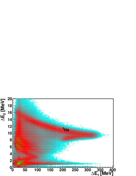
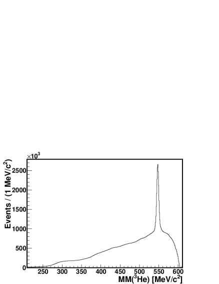
Figure 1: (left) Correlation of energy deposits between two Forward Detector plastic detector layers: the first thick layer (11 cm), $\Delta E_{1}$, and a preceding thin (0.5 cm) layer, $\Delta E_{2}$. (right) MM($\mbox{}^{3}\mbox{He}$) for all events with a $\mbox{}^{3}\mbox{He}$ detected in the FD. There are about $1.2\cdot 10^{7}$ events in the peak corresponding to the $pd\to\mbox{}^{3}\mbox{He}\eta$ reaction.

The missing mass calculated from the reconstructed ³He momentum, MM($\mbox{}^{3}\mbox{He}$), is shown in Fig. 1(right). The $\eta$ peak has a width of 6.2 MeV$/c^{2}$ (FWHM) and contains about $1.2\cdot 10^{7}$ events. The luminosity during the run was kept in range $(1-5)\times 10^{31}$ cm^-2s^-1.

II.2 Simulation

The measurement of the production reaction $pd\to\mbox{}^{3}\mbox{He}\eta$ is simulated by using the experimental angular distribution from Bilger et al. (2002); Rausmann et al. (2009). The decay $\eta\rightarrow\pi^{+}\pi^{-}\pi^{0}$ (BR=22.92(28)% Beringer et al. (2012)) was simulated at the final stage using the central values of the extracted experimental Dalitz plot parameters. The main physics background processes include the $\eta\to\pi^{+}\pi^{-}\gamma$ (BR=4.22(8)% Beringer et al. (2012)) decay and the direct two and three pion production reactions: $pd\rightarrow\mbox{}^{3}\mbox{He}\pi^{+}\pi^{-}$, $pd\rightarrow\mbox{}^{3}\mbox{He}\pi^{+}\pi^{-}\pi^{0}$. For the $\eta\rightarrow\pi^{+}\pi^{-}\gamma$ we used the results reported in Adlarson et al. (2012); Babusci et al. (2013b). All other $\eta$ decay channels contribute marginally to the final result and may therefore be neglected. The direct 3$\pi$ production channel simulated with uniform phase space distributions were modified to reproduce our final MM($\mbox{}^{3}\mbox{He}$) distribution as extracted from Fig. 3.

The chance coincidental events for the 16 most prominent $pd$ reaction channels (total cross section 80 mb) and the effect of energy pile-up in the different detector elements are also included in the simulation. Their relative strengths of the different channels are assumed using the Fermi statistical model. For the quasi-free break up reactions the relative momentum between the np-pair is simulated using the deuteron wave function is used while for all other channels uniform phase space is assumed.

The accelerator and the target pellet beam overlap region is 3.8 mm in the horizontal and 5 mm in the vertical direction. The interaction point distribution can have tails in the $z$-direction since the accelerator beam can also interact with a small fraction of the surrounding rest gas or divergent pellets. The shape of the tails is based on the $z$-vertex distribution deduced from experimental data with $\mbox{}^{3}\mbox{He}$ production.

II.3 Event selection

The signature of an event, in addition to the $\mbox{}^{3}\mbox{He}$ ion reconstructed in FD, is at least two tracks from charged particles in the MDC and at least two clusters in the calorimeter not associated with the tracks. The polar angles of charged particles detected in the MDC are larger than $30^{\circ}$ and less than $150^{\circ}$. The time window in the CD with respect to the time signal of the $\mbox{}^{3}\mbox{He}$ is 6.2 ns for the charged particle tracks and 30 ns for neutral particle hit. All possible combinations of tracks are retained for kinematic fitting even if the number of tracks in the event is greater than the expected number of final state particles.

The point of closest approach of the two charged particle tracks of the CD should be within 7 cm from the center of the pellet and COSY beams overlap region. A kinematic fit with the

$$pd\rightarrow\mbox{}^{3}\mbox{He}\pi^{+}\pi^{-}\gamma\gamma$$ (5)

reaction hypothesis is applied and the combination with the lowest $\chi^{2}$ value is selected. A cut on the $\chi^{2}$ probability is made at 1%. In the remaining analysis the variable values adjusted by the fit are used. The correlation between the fitted MM$(^{3}\textrm{He})$ and the invariant mass of the two photons, IM$(\gamma\gamma)$, is shown in Fig. 2(left).

Fig. 2(right) shows the extracted yield of the $pd\to\mbox{}^{3}\mbox{He}\eta$ events as a function of IM$(\gamma\gamma)$. The distribution was obtained by creating 2 MeV/c² horizontal slices of the scatter plot in Fig. 2(left) and determining the peak content of each one. The resulting distribution agrees well with simulations of the $\eta\to\pi^{+}\pi^{-}\pi^{0}$ and $\eta\to\pi^{+}\pi^{-}\gamma$ decays. The relative normalization between the two decays is fixed by their branching ratios. For the final data sample only events with IM$(\gamma\gamma)>100$ MeV/c² are selected.

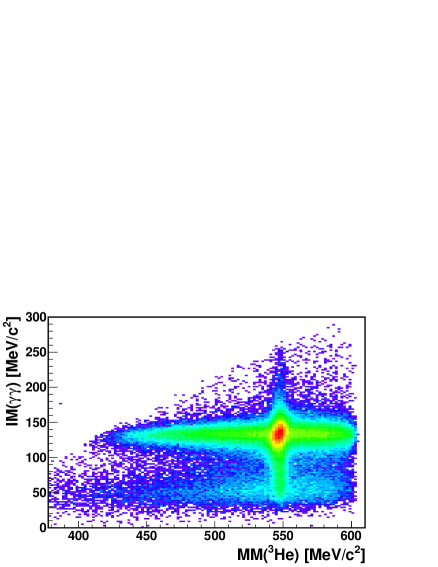
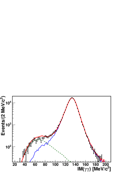
Figure 2: (left) Correlation between MM$(^{3}\textrm{He})$ and IM$(\gamma\gamma)$ for variables adjusted by a kinematic fit. (right) Comparison of the experimental and simulated contributions of the $\eta$ events as the function of IM$(\gamma\gamma)$. The extracted number of the events in the $\eta$ peak for each 2 MeV/c² IM$(\gamma\gamma)$ slice is well described by the simulation (thick solid red line) including the $\eta\to\pi^{+}\pi^{-}\pi^{0}$ (solid blue line) and $\eta\to\pi^{+}\pi^{-}\gamma$ decays (dashed green line).

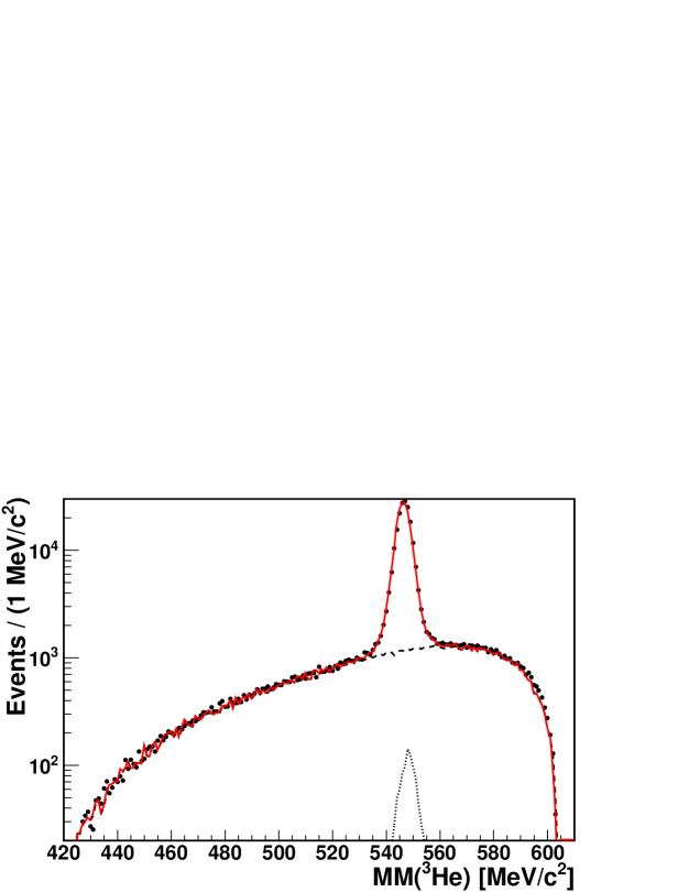
Figure 3: The distribution of MM$(\mbox{}^{3}\mbox{He})$ using variables adjusted by the kinematic fit for the final data sample (dots), agree well with the sum of the Monte Carlo distributions for the signal and the backgrounds (red solid line). Separately are shown contributions from $\eta\rightarrow\pi^{+}\pi^{-}\gamma$ (dotted line) and from the direct $3\pi$ production (dashed line).

The data sample used in this analysis consists of $1.74\cdot 10^{5}$ $\eta$ candidates. The comparison of the simulated and experimental distributions of MM$(\mbox{}^{3}\mbox{He})$ is shown in Fig. 3. The dominating background comes from direct three pion production. The contributions from two pion production and the $\eta\to\pi^{+}\pi^{-}\gamma$ decay are less than 1$\%$.

III Results

The variables $X$ and $Y$ are calculated from Eqn. (2) using the kinetic energies of the charged pions after the kinematic fitting boosted to the rest frame of the $\pi^{+}\pi^{-}\gamma\gamma$ system. For the variables after the kinematic fit of the reaction (5) one has $\mu\equiv\mbox{IM}(\pi^{+}\pi^{-}\gamma\gamma)=\mbox{MM}(^{3}\mbox{He})$. However, $\mu$ is not constrained to equal $m_{\eta}$ and IM$(\gamma\gamma)$ not constrained to $m_{0}$. Therefore, the kinetic energy of the neutral pion, $T_{0}$, is determined in the following way:

$$T_{0}=\mu-T_{+}-T_{-}-2m_{\pm}-\mbox{IM}(\gamma\gamma),$$ (6)

and for calculating $Q_{\eta}$ we use Eqn. (3).

The selected Dalitz plot bin width in $X$ and $Y$ ($\Delta X=\Delta Y=0.2$) is in our case limited by the statistics needed for background subtraction and reliable systematical crosschecks. The uncertainty of the $X$ and $Y$ measurement is well within the experimental resolution (FWHM of approximately 0.10 for both $\Delta X$ and $\Delta Y$ in average). The $X,Y$ region $[-1.1,1.1]\times[-1.1,1.1]$ is divided into $11\times 11$ bins. The border bins with less than 90% Dalitz plot area inside the kinematic boundaries are excluded leading to 59 bins used in the analysis. Definition and the numbering scheme of the bins is given in Fig. 4.

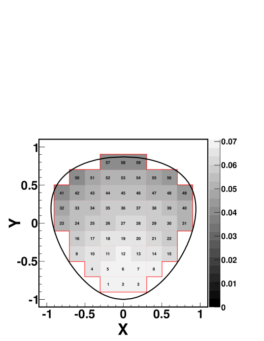
Figure 4: Position and numbering of the Dalitz plot bins used for the analysis. The acceptance for the $\eta\to\pi^{+}\pi^{-}\pi^{0}$ decay is also indicated by the gray scale.

The Dalitz plot for the $\eta\to\pi^{+}\pi^{-}\pi^{0}$ decay is obtained by dividing the reconstructed $X$ and $Y$ variables into bins and determining the signal content in each bin from the corresponding $\mu$ distribution. The signal content in each bin is estimated by a least squared fit of the simulated data of $pd\to\mbox{}^{3}\mbox{He}\eta$ and the $pd\to\mbox{}^{3}\mbox{He}\pi^{+}\pi^{-}\pi^{0}$ continuum background reaction. The matrix element squared of the background reaction is assumed to be a linear function of $\mu$:

$$F_{i}(\mu)=N_{S}^{i}s_{i}(\mu)+N_{B}^{i}\left(1+\alpha_{i}\mu\right)b_{i}(\mu),$$ (7)

where $i$ is the Dalitz plot bin number, $N_{S}^{i}$ is the normalization factor for the simulated $pd\to\mbox{}^{3}\mbox{He}\eta$ signal, $s_{i}(\mu)$. $N_{B}^{i},b_{i}(\mu)$ have the corresponding meaning with respect to the flat phase space simulation of the $pd\to\mbox{}^{3}\mbox{He}\pi^{+}\pi^{-}\pi^{0}$ reaction. $N_{S}^{i}$, $N_{B}^{i}$ and $\alpha_{i}$ are free parameters in the fit.

Two examples of the fits are shown in Fig. 5; one for a Dalitz plot bin with larger statistics (bin #2, centered at $X=0$, $Y=-0.8$) and one for a bin with lower statistics, (bin #53, centered at $X=0$, $Y=0.6$).

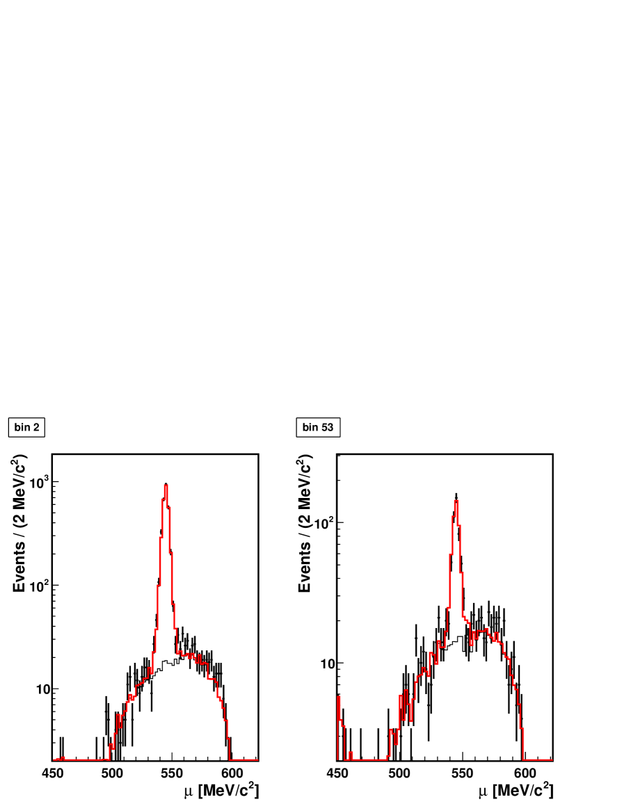
Figure 5: Two examples of the fits to the $dN/d\mu$ distributions for a large (left) and a low statistics Dalitz plot bin (right). The red thick line is the fitted function Eq. 7 while the thin line represents the continuous background contribution.

Finally the simulated background from $\eta\to\pi^{+}\pi^{-}\gamma$ events is subtracted from $N_{S}^{i}$. This contribution is small compared to the statistical uncertainties. The extracted number of $\eta\to 3\pi$ events is corrected for acceptance. It was checked that the use of bin by bin acceptance correction (i.e. diagonal smearing matrix) does not introduce any significant systematic effect.

The acceptance values, indicated in Fig. 4, are obtained from a MC sample of $5\cdot$10⁷ $\eta\to\pi^{+}\pi^{-}\pi^{0}$ events and varies between 4% and 7%. It is larger when $T_{0}$ is small (i.e. lower $Y$-values), but also when the kinetic energies of the two charged pions are similar (i.e. for $X$ close to zero). Fig. 6 shows the acceptance corrected number of $\eta\rightarrow\pi^{+}\pi^{-}\pi^{0}$ events as function of the Dalitz plot bin number.

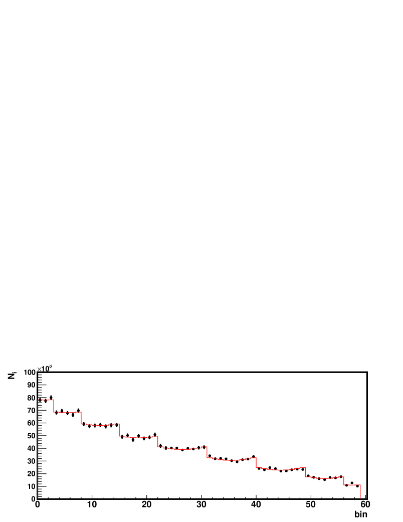
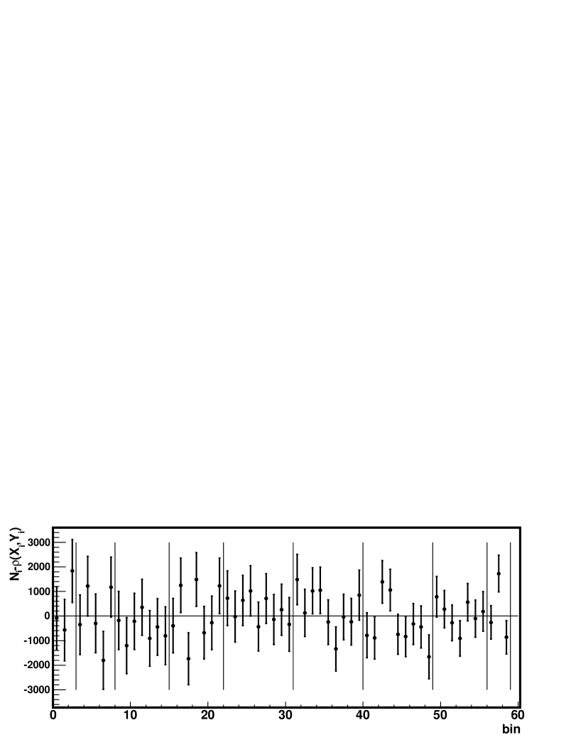
Figure 6: The upper panel shows acceptance corrected Dalitz plot bin contents with statistical uncertainties (black points with error bars) compared to the fitted function $\rho(X,Y)$ (red line) for each bin. The lower panel shows the corresponding residuals.

The Dalitz plot parameters are obtained with the least square fitting procedure which minimizes

$$\chi^{2}=\sum^{59}_{i=1}\left(\frac{N_{i}-\rho(X_{i},Y_{i})}{\Delta N_{i}}\right)^{2}.$$ (8)

$N_{i}$ and $\Delta N_{i}$ denote the acceptance corrected number of events and their statistical uncertainty for the Dalitz plot bins $i=1,..,59$). The function $\rho(X_{i},Y_{i})$, defined in Eqn. (4), is evaluated at the center of each Dalitz plot bin: $X_{i}$ and $Y_{i}$. In our case the systematic effects introduced by this procedure are negligible as it was checked using MC data sample. The overall normalization factor $N$ is also a free parameter in the fit.

The obtained Dalitz plot parameters together with their statistical uncertainties are presented in Tab. 3 for different assumptions about the Dalitz plot parameters together with the fit $\chi^{2}$ and number of degrees of freedom (dof). The $c$ and $e$ parameters are fixed to $0$ in the fits. In addition we have performed fits including these parameters. The result gives $c$ and $e$ consistent with zero: $c=-0.007(9)$ and $e=-0.020(23)$ and does not affect other parameters. For the case when all $a$, $b$, $c$, $d$, $e$ and $f$ parameters are fit one obtains $\chi^{2}/dof=46.6/52$. The correlation matrix between the fitted parameters for the standard result obtained is shown in Tab. 4.

	$a$	$b$	$d$	$f$	$\chi^{2}/dof$
4 parameters (std)	$-1.144(18)$	0.219(19)	0.086(18)	0.115(37)	49.4 / 54
3 parameters	$-1.101(11)$	0.234(19)	0.078(18)	0 (fix)	58.8 / 55
2 parameters	$-1.075(9)$	0.201(17)	0 (fix)	0 (fix)	78.3 / 56

Table 3: Fit results for different sets of Dalitz plot parameters. The normalization factor, $N$, is omitted from the table. A number followed by ’(fix)’ means that the corresponding parameter was fixed to this number.

	a	b	d
b	$-0.24$
d	$-0.45$	$0.36$
f	$-0.79$	$-0.25$	$0.14$

Table 4: Correlation matrix for the Dalitz plot parameters.

Tab. 4 shows a strong anti-correlation between the parameter $a$ and $f$ which is also reflected in the uncertainties of the parameter $a$. The bins of the Dalitz plot are compared in Fig. 6 to the parametrization with four free parameters $a,b,d,f$ where the remaining ones are set to zero (parametrization labeled as std in Tab. 3).

IV Systematic uncertainties

The systematic uncertainties of the obtained Dalitz plot parameters are investigated by including variations due to know sources of uncertainties in the MC generated data and by changing the selection criteria to find the remaining effects. In particular the consistency of extraction of the Dalitz plot distribution and fitting of the Dalitz plot parameters were tested using MC generated data ten times larger than in the experiment. The input parameters were reproduced without introducing any systematical deviation within the statistical uncertainties.

One of the most important sources of systematical uncertainties is the direct background subtraction procedure. This uncertainty is estimated by comparing a fit with the signal region excluded from the fit and the signal term $N_{S}^{i}s_{i}(\mu)$ in Eqn. (7) is omitted and the background is subtracted directly from the data ([Test 1] in Tab. 5).

To investigate further possible systematical effects the data sample has been divided into sets of high and low luminosity. The $pd\rightarrow X$ cross section is $\sim$ 80 mb, which amounts to few background reactions produced per $\mu s$. The largest effect is connected to the calorimeter signals since the decay times are of the order of $\mu s$. The Dalitz plot parameter values obtained for the low and high luminosity sample are shown by [Test 2] in Tab. 5.

Two different accelerator beam modes were used during the beam time and they cover roughly equal time of data taking. In the first half, a constant beam energy during the accelerator cycle was assured by a fixed radio frequency (RF). In the second half, a coasting beam with RF switched off swept the target leading to a slight decrease of the beam energy during a cycle (from 1000.0 MeV to 993.5 MeV). In the experimental analysis this energy decrease is taken into account. However, in the simulations the acceptance has been calculated for a beam kinetic energy fixed at 1 GeV. The comparison of the two cases ([Test 3] in Tab. 5) shows the largest deviation for the $b$ parameter ($\approx$ 2$\sigma$). To investigate the source of the effect we have calculated the acceptances also for the lowest beam energy in the RF off mode (993.5 MeV) and concluded that the change is too small to explain the observed deviation.

The effect of the uncertainty of the implemented detector resolution in the detector simulations is tested by increasing the kinematic fit probability from 0.01 to 0.1 ([Test 4] in Tab. 5). The difference between the parameter values are not significant and are therefore neglected in the final systematical uncertainty.

	$-a$	b	d	f	$\chi^{2}$ / $d.o.f.$
Standard result	1.144(18)	0.219(19)	0.086(18)	0.115(37)	49.4 / 54
[Test 1] Background fit	1.126(18)	0.230(19)	0.094(18)	0.111(37)	60.5 / 54
[Test 2] Low luminosity	1.130(24)	0.216(26)	0.059(24)	0.104(50)	50.5 / 54
[Test 2] High luminosity	1.164(25)	0.219(28)	0.106(26)	0.152(52)	54.9 / 54
[Test 3] RF	1.127(26)	0.177(28)	0.085(27)	0.140(55)	56.1 / 54
[Test 3] No RF	1.139(23)	0.252(26)	0.076(24)	0.069(49)	49.6 / 54
[Test 4] PDF$>0.1$	1.146(22)	0.224(24)	0.075(22)	0.117(46)	48.0 / 54

Table 5: Dalitz plot parameters extracted for different tests for systematic effects. Description in the text.

The only significant changes are seen for the $b$ parameter for the two accelerator operation modes and for $d$ for the two luminosity cases. We use metodology of Ref. Barlow (2002) and express the final result for the Dalitz plot parameters in the following way:

$$-a = 1.144\pm 0.018(stat)$$

$$b = 0.219\pm 0.019(stat)\pm 0.037(syst)$$

$$d = 0.086\pm 0.018(stat)\pm 0.018(syst)$$

$$f = 0.115\pm 0.037(stat).$$

In addition we give the values for the C violating parameters $c$ and $e$:

$$c = -0.007\pm 0.009(stat)$$

$$e = -0.020\pm 0.023(stat)\pm 0.029(syst).$$

The results are dominated by statistical uncertainties and therefore the provided table with acceptance corrected bin contents, Tab. 6, could be used directly for comparison with theoretical models.

V Discussion of results

Parameters $a$, $b$ and $d$ significantly deviate from zero. The $d$ parameter is 3.4$\sigma$ above zero. From Tab. 3 it is seen that $\chi^{2}$ per dof is only slightly worse if parameter $f$ is set to zero in the fit. The significance of allowing $f\neq 0$ in our data is 3.1$\sigma$. However, the $a$ and $f$ parameters are strongly anti-correlated (see Tab. 4) and excluding $f$ from the fit affects also the $a$ value. The data do not require higher order terms in the polynomial expansion such as $g\cdot X^{2}Y$ and $h\cdot X^{3}$.

Here we list deviations from the Dalitz plot parameters obtained by the KLOE collaboration Ambrosino et al. (2008) together with their significance (statistical and systematic uncertainties are added in squares):

$$-\Delta a = +0.054(23)\ \ (+2.3\sigma)$$

$$\Delta b = +0.095(44)\ \ (+2.2\sigma)$$

$$\Delta d = +0.029(28)\ \ (+1.0\sigma)$$

$$\Delta f = -0.025(43)\ \ (-0.6\sigma).$$

Our results are generally consistent with KLOE, however there is some tension for $a$ and $b$ parameters. Our data confirm the discrepancies between theoretical calculations and the experimental values from the KLOE experiment. The provided experimental data points of the individual Dalitz plot bins will allow independent analyses using NREFT or dispersive methods.

The presented results are based on a first part of the WASA-at-COSY data from the $pd\to^{3}\textrm{He}\eta$ reaction. More data are available from WASA-at-COSY also from the $pp\to pp\eta$ reaction. Together with expected results from other experiments the goal of a precise determination of the $\eta\to\pi^{+}\pi^{-}\pi^{0}$ Dalitz plot parameters might soon be reached.

Bin #	Content	Bin#	Content	Bin #	Content	Bin #	Content
1	2.020 $\pm$ 0.033	16	1.271 $\pm$ 0.029	31	1.058 $\pm$ 0.028	46	0.573 $\pm$ 0.021
2	2.004 $\pm$ 0.032	17	1.296 $\pm$ 0.029	32	0.883 $\pm$ 0.027	47	0.597 $\pm$ 0.022
3	2.069 $\pm$ 0.033	18	1.209 $\pm$ 0.027	33	0.824 $\pm$ 0.025	48	0.611 $\pm$ 0.022
4	1.764 $\pm$ 0.031	19	1.289 $\pm$ 0.028	34	0.830 $\pm$ 0.024	49	0.604 $\pm$ 0.023
5	1.794 $\pm$ 0.031	20	1.236 $\pm$ 0.028	35	0.820 $\pm$ 0.024	50	0.473 $\pm$ 0.021
6	1.752 $\pm$ 0.031	21	1.257 $\pm$ 0.028	36	0.783 $\pm$ 0.024	51	0.443 $\pm$ 0.020
7	1.716 $\pm$ 0.031	22	1.313 $\pm$ 0.029	37	0.758 $\pm$ 0.023	52	0.418 $\pm$ 0.019
8	1.804 $\pm$ 0.032	23	1.085 $\pm$ 0.029	38	0.802 $\pm$ 0.024	53	0.398 $\pm$ 0.019
9	1.528 $\pm$ 0.031	24	1.042 $\pm$ 0.027	39	0.815 $\pm$ 0.025	54	0.440 $\pm$ 0.020
10	1.484 $\pm$ 0.029	25	1.041 $\pm$ 0.026	40	0.867 $\pm$ 0.026	55	0.433 $\pm$ 0.020
11	1.499 $\pm$ 0.030	26	1.041 $\pm$ 0.026	41	0.626 $\pm$ 0.024	56	0.458 $\pm$ 0.021
12	1.511 $\pm$ 0.030	27	1.000 $\pm$ 0.026	42	0.600 $\pm$ 0.022	57	0.283 $\pm$ 0.018
13	1.481 $\pm$ 0.029	28	1.033 $\pm$ 0.026	43	0.641 $\pm$ 0.022	58	0.331 $\pm$ 0.019
14	1.504 $\pm$ 0.030	29	1.021 $\pm$ 0.026	44	0.622 $\pm$ 0.022	59	0.268 $\pm$ 0.018
15	1.512 $\pm$ 0.030	30	1.049 $\pm$ 0.027	45	0.572 $\pm$ 0.021

Table 6: Acceptance corrected Dalitz plot distribution. The bin numbering is given in Fig. 4. The bin contents are normalized to the bin centered at $X=0,Y=0$ (bin #27).