Beyond correlation in spatial statistics modeling

Abstract

We introduce a model for spatial statistics which can account explicitly for interactions among more than two field components at a time. The theoretical aspects of the model are dealt with: cumulant and moment generating functions, spatial consistency and parameter estimation. On the basis of a detailed synthetic example, we show the kind of inference about the (partially observed) spatial field that can be very wrong, if one validates his model by checking only one and two dimensional marginal fit, and covariance function fit. We suggest statistics that can be used additionally for model validation, which help assess interdependence among groups of variables. The implications of considering multivariate interactions for intense daily precipitation forecasting over a small catchment in southeastern Germany (that of the Saalach river) are investigated.

1 Introduction

In the context of precipitation downscaling, Bárdossy and Pegram [2012] found that observed clustering patterns of very high values at multiple locations on the target scale could not be reproduced by simulated data, even after site-wise (i.e. marginal) bias correction and correlation bias correction of the simulations. That is, even though the marginal distributions and the inter-site correlations of the data simulated for the validation period were identical to those of observed data in the same period, clustering patterns of observed data were still not properly recovered, particularly for clusters with very high values: the data simulated were unable to recover the distribution of the sum of blocks of four sites or “pixels”. This may lead to substantial underestimation of flood return periods, since the occurrence of unexpected clusters of intense rainfall over a catchment can result in great floods, not expected in centuries.

The paper of Bárdossy and Pegram [2012] adds evidence to that of Bárdossy and Pegram [2009] about the need to build spatial models which can consider, explicitly, simultaneous interactions among more than two of the components of the modeled field. The present paper proposes one such model, and elaborates on its theory. It is conceived as an initial step in a research direction which has gone mostly unnoticed. It intends to help start a wider discussion on the topic of multivariate interactions for spatial statistics models.

In our exposition, we focus for simplicity on the class of second order stationary processes, possibly after subtracting a trend field. We also assume a two dimensional isotropic field, and that the studied spatial process takes values only on a finite number of locations over a grid. However, these simplifications are by no means restrictive of the methodology presented in this paper; they just help to make exposition easier.

Consider spatially labeled locations $\left\{\mathbf{s_{1}},\mathbf{s_{2}},\ldots,\mathbf{s_{J}}\right\}$,with $\mathbf{s_{j}}\in\mathbb{R}^{2}$, and let

$$\left(\mathbf{Z\left(s_{1}\right)},\mathbf{Z\left(s_{2}\right)},\ldots,\mathbf{Z\left(s_{J}\right)}\right)$$

represent a random quantity taking values at the given locations, so that a field of variable $\mathbf{Z}$ is obtained. Association between every two components of this field can be modeled in terms of covariance function, $C$,

$$cov\left(\mathbf{Z\left(s_{i}\right),}\mathbf{Z\left(s_{j}\right)}\right)=C\left(\left\|\mathbf{s_{i}}-\mathbf{s_{j}}\right\|\right)$$ (1)

where $\left\|\mathbf{s_{i}}-\mathbf{s_{j}}\right\|$ is the euclidean distance between $\mathbf{s_{i}}$ and $\mathbf{s_{j}}$. This covariance function must ensure positive-definiteness of the resulting covariance matrix. For example, two popular covariance functions are:

Powered-exponential:

given by equation

$$C\left(d\right)=\sigma_{0}^{2}.I\left(d=0\right)+\sigma_{1}^{2}\exp\left(-\left(d/\theta_{1}\right)^{\theta_{2}}\right)$$ (2)

where $I\left(*\right)$ stands for the indicator function.

Matérn’s:

given by equation

$$C\left(d\right)=\sigma_{0}^{2}.I\left(d=0\right)+\sigma_{1}^{2}\left[2^{\theta_{2}-1}\Gamma\left(\theta_{2}\right)\right]^{-1}\left[d/\theta_{1}\right]^{\theta_{2}}K_{\theta_{2}}\left(d/\theta_{1}\right)$$ (3)

where $\Gamma\left(*\right)$ stands for the Gamma function and $K_{\theta_{2}}\left(d/\theta_{1}\right)$ for the modified Bessel function of the second kind of order $\theta_{2}$ (see, for example Abramowitz [1972]).

Parameters $\left(\theta_{1},\theta_{2},\sigma_{0}^{2},\sigma_{1}^{2}\right)$ are the covariance function parameters. Hence, only a reduced number of parameters must be estimated in order to find the covariance between every two components $\mathbf{Z\left(s_{i}\right)}$ and $\mathbf{Z\left(s_{j}\right)}$, given locations $\mathbf{s_{i}}$ and $\mathbf{s_{j}}$.

The Normal model is a common model in Spatial Statistics for components corresponding to every finite set of locations,

$$\left(\mathbf{Z\left(s_{1}\right),}\ldots,\mathbf{Z\left(s_{J}\right)}\right)\sim N_{J}\left(\mu,\Sigma\right)$$

where the covariance matrix is given by $\Sigma_{ij}=C\left(\left\|\mathbf{s_{i}}-\mathbf{s_{j}}\right\|\right)$. Under the Gaussian model, the whole distribution is defined by a vector of means $\mu\in\mathbb{R}^{J}$ and parameters $\left(\theta_{1},\theta_{2},\sigma_{0}^{2},\sigma_{1}^{2}\right)$, which determine matrix $\Sigma$. It is often the case that the mean vector is represented as a function $\xi$ of the geographic coordinates of $\mathbf{s_{j}}$, or of an additional variable ("external drift") related to such location ,

$$\mu_{j}=\xi\left(\mathbf{s_{j}}\right)$$ (4)

For a new location $\mathbf{s_{k}}\notin\left\{\mathbf{s_{1},s_{2},s_{3},\ldots,s_{J}}\right\}$, the joint distribution of

$$\left(\mathbf{Z\left(s_{1}\right),}\ldots,\mathbf{Z\left(s_{J}\right)},\mathbf{Z\left(s_{k}\right)}\right)$$

can be readily found under the Normal model: one adds component $\mu_{k}=\xi\left(\mathbf{s_{k}}\right)$ to the means vector, and extends the covariance matrix by $\Sigma_{ik}=C\left(\left\|\mathbf{s_{i}}-\mathbf{s_{k}}\right\|\right)$, for each $\mathbf{s_{i}}\in\left\{\mathbf{s_{1},s_{2},s_{3},\ldots,s_{J}}\right\}$. The model is thus completely specified. This is one of the reasons why the Normal model is very convenient conceptually, and is often used in practice, if necessary after applying a suitable transformation to data (see section 6).

The family of elliptical distributions can be seen as the wider family to which both the multivariate Normal and the multivariate Student distributions belong. The classical definition, according to Cambanis et al. [1981], is as follows:

Definition

Let $\mathbf{X}$ be a J-dimensional random vector, $\mu\in\mathbb{R}^{J}$ and $\Sigma$ a $J\times J$, non-negative definite matrix. Let $\phi_{\mathbf{X}-\mu}\left(\mathbf{t}\right):\mathbb{R}^{J}\rightarrow\left[0,+\infty\right)$ be the characteristic function of $\mathbf{X}-\mu$. If $\phi_{\mathbf{X}-\mu}\left(\mathbf{t}\right)=\Psi\left(\mathbf{t}\Sigma\mathbf{t^{{}^{\prime}}}\right)$ for some function $\Psi\left(s\right):\left[0,+\infty\right)\rightarrow\left[0,+\infty\right)$, then we say that $\mathbf{X}$ has an elliptically contoured distribution with parameters $\mu$ and $\Sigma$.

In case $\mathbf{X}-\mu$ is Normally distributed with means vector $\mathbf{0}$ and covariance matrix $\Sigma$, one has of course $\Psi\left(s\right):=\exp\left(-\frac{1}{2}s\right)$.

An elliptically distributed vector $\mathbf{X}-\mu$ can always be represented as

$$\mathbf{X}-\mu=R\times\mathbf{U}\times\Sigma^{\frac{1}{2}}$$ (5)

where $\Sigma^{\frac{1}{2}}$ is a $J\times J$ matrix such that $\Sigma^{\frac{1}{2}}\times\mbox{$\left(\Sigma^{\frac{1}{2}}\right)^{T}$}=\Gamma$, for example its Cholesky decomposition factor; $R\geq 0$ is a non-negative random variable; and $\mathbf{U}\in\mathbb{R}^{J}$ is a random vector uniformly distributed on the boundary of the unit hypersphere (see Cambanis et al. [1981]). Variable $R$ receives the name of “generating variable”, and together with $\Sigma$ determines the specific characteristics of $\mathbf{X}$, most importantly, its tail behavior. The generating variable is what really marks the difference among the several elliptical distributions one might construct.

Example 1

In case $\mathbf{X}-\mu$ is Normally distributed with means vector $\mathbf{0}$, then generating variable $R$ is distributed as a $\chi$ distribution with $J$ degrees of freedom. That is, $R^{2}\sim\chi_{J}^{2}$, a chi-squared distribution with $J$ degrees of freedom.

Another well-known case is that of the multivariate student distribution with $\nu$ degrees of freedom, for which $R^{2}\sim J\times F_{J,\nu}$, and $F_{J,\nu}$ represents the Fisher distribution with $J$ and $\nu$ degrees of freedom.

Despite being a generalization to the Normal model, which pervades the Spatial Statistics literature, elliptical models are not part of current practice in the area. For example, among other excellent books on the subject, no mention is made about elliptical distributions at Le and Zidek [2006], Cressie and Wikle [2011], Cressie [1991], Diggle and Ribeiro [2007], Banerjee et al. [2003]. This may have to do with the inconvenient the model presents for interpolation or “kriging”: For the multivariate Normal and student models, it has already been seen that the distribution of the generating variable depends on the dimension of the vector $\mathbf{X}\in\mathbb{R}^{J}$, which means that function $\Psi$ must also change. Since our model is defined in terms either of $\Psi$, as in definition 1, or in terms of generating variable $R$, as in representation (5), it is not clear in general into what these parameters will turn when extending the model to $k$ “ungauged” sites, whereby $\mathbf{X}\in\mathbb{R}^{J+k}$. This issue is addressed in this paper.

Our intention in dealing with elliptical distributions is to consider interdependence among variables that cannot be quantified in terms of correlations or covariances alone, which concepts form the core of dependence modeling in current spatial statistical practice. The topic of "beyond correlation interdependence" has been addressed in itself by Rodríguez and Bárdossy [2013]. We intend here to give an implementation to the ideas presented at Rodríguez and Bárdossy [2013] in the context of Spatial Statistics.

At Rodríguez and Bárdossy [2013], a distinction is drawn between interaction “parameters”, and interaction “manifestations”. The latter are subject-matter specific statistics connected with sub-vectors of the analyzed random vector, $\mathbf{X}$, and dependent on the type of association among the components of such sub-vectors; they have a relevant interpretation for the researcher. Interaction “parameters” can be seen as convenient building blocks of a (low dimensional) model or dependence structure that can somehow reproduce the target interaction manifestations. It is argued that the joint cumulants of $\mathbf{X}$ are legitimate extensions to correlation coefficients to more than two variables, and as the building blocks referred to above. The cumulant generating function is then accordingly referred to as a “dependence structure”.

In the present paper, we show how we can build a low dimensional (regarding the number of parameters to fit) spatial model on the basis of joint cumulants, i.e. on the basis of a cumulant generating function. This model can be considered a natural extension to the Normal model. A Normal model is built on the order one and two joint cumulants only, namely a means vector $\mu$ containing the order one cumulants, and an array of covariances $cov\left(X_{j},X_{i}\right)$ containing the order two joint cumulants. In the extension here presented, higher order joint cumulants can be considered without increasing prohibitively the number of parameters to fit.

The rest of the paper is structured as follows. Section 2 is theoretical; it introduces our model via its cumulant generating function; it is intended to make clear why the model actually considers interactions among groups of variables with a minimum of parameters. Section 3 is a transition toward practical applicability; it shows the probability density of the model, and how to ensure spatial consistency; a basic parameter estimation procedure is presented. Section 4 shows how to obtain unconditional realizations of the field for arbitrary dimensions, how to find conditional distributions given partial observations of the field, and how to simulate conditional fields of an arbitrary dimension. Section 5 can be considered the core of this paper; by means of a synthetic example, it explores the kind of inference that can go wrong when using a model predicated on a combination of bi-variate connections only; it also suggests some statistics that can help to identify interdependence features of data beyond correlation. Section 6 analyzes the implications of multivariate interdependence for flood risk assessment in the Saalach river catchment, in southeastern Germany; a space-time model, whose structure is provided by a latent Gaussian field, is fitted to daily precipitation from 2004 to 2009; this latent Gaussian structure is replaced by a quasi-Gaussian structure which possesses interactions beyond correlations, and the forecasts of the two versions are compared; in addition, the conditional rainfall field of June 1st 2013 over the catchment is analyzed in the light of both models. Section 7 contains a short discussion and intended future work.

2 The proposed model

In the following, we assume the existence of sufficiently many product moments of $\mathbf{X}$; sufficient so as to provide a practically useful approximation to the processes modeled. Then it is more convenient, for our purposes, to conceptualize elliptical distributions in terms of their moment generating function.

It might be protested that moments (and hence cumulants) of sufficiently high orders might not exist for the “true” probability distribution of the process under analysis. We would answer that such distributions can always be sufficiently (i.e. for practical purposes) approximated by a distribution with existing moments of all orders. See, for example Gallant and Nychka [1987], where the authors introduce a semi-parametric model, similar to an Edgeworth expansion. This model possesses moments of all orders. Yet, under minimal conditions it can approximate any continuous distribution on $\mathbb{R}^{J}$, provided sufficiently many factors are added to the sum defining the model. Additionally, Del Brio et al. [2009], Mauleon and Perote [2000], Perote [2004] present variants of the model of Gallant and Nychka [1987], and show how they can be effectively applied to modeling heavy tailed data, both univariate and multivariate.

We say, then, that random vector $\mathbf{X}\in\mathbb{R}^{J}$ is “elliptically distributed” if and only if its moment generating function can be written as

$$M_{\mathbf{X}-\mathbf{\mu}}\left(\mathbf{t}\right)=E\left(e^{\left\langle\mathbf{t},\mathbf{X}-\mu\right\rangle}\right)=\Upsilon\left(\mathbf{t^{T}}\text{$\Sigma$}\mathbf{t}\right)$$ (6)

for some function $\Upsilon:\mathbb{R}\rightarrow\mathbb{R}$, and some $\mathbf{\mu}\in\mathbb{R}^{J}$. For the sake of simplicity, we assume for now that $\mu=\mathbf{0}$.

Consider a moment generating function of the form

$$M_{\mathbf{X}}\left(\mathbf{t}\right)=\exp\left(\delta\left(\frac{1}{2}\mathbf{t^{T}}\Sigma\mathbf{t}\right)\right)$$ (7)

for some function $\delta:\mathbb{R}\rightarrow\mathbb{R}$. Then the cumulant generating function (c.g.f.) of $\mathbf{X}$ is given by

$$K_{\mathbf{X}}\left(\mathbf{t}\right):=\log\left(M_{\mathbf{X}}\left(\mathbf{t}\right)\right)=\delta\left(\frac{1}{2}\mathbf{t^{T}}\Sigma\mathbf{t}\right)$$ (8)

This function $\delta\left(y\right)$ can be formally expanded in its Taylor Series around zero,

$$\delta\left(y\right)=c_{0}+\frac{c_{1}}{1!}y+\frac{c_{2}}{2!}y^{2}+\frac{c_{3}}{3!}y^{3}+\frac{c_{4}}{4!}y^{4}+\ldots\\ =c_{0}+\frac{c_{1}}{1!}\left(\frac{1}{2}\mathbf{t^{T}}\Sigma\mathbf{t}\right)+\frac{c_{2}}{2!}\left(\frac{1}{2}\mathbf{t^{T}}\Sigma\mathbf{t}\right)^{2}+\frac{c_{3}}{3!}\left(\frac{1}{2}\mathbf{t^{T}}\Sigma\mathbf{t}\right)^{3}+\ldots\\ =\delta\left(\left(\frac{1}{2}\mathbf{t^{T}}\Sigma\mathbf{t}\right)\right)$$ (9)

where $c_{r}=\frac{d^{r}}{dy^{r}}\delta\left(y\right)\mid_{y=0}$.

A little thought shows that the assumption $\mathbf{\mu}=\mathbf{0}$ implies that $c_{0}=0$. Thus, by virtue of (8) and (9) combined, we have that the c.g.f can be written as

$$K_{\mathbf{X}}\left(\mathbf{t}\right)=c_{1}\frac{1}{2}\mathbf{t^{T}\Sigma t}+\frac{1}{2!}c_{2}\left[\frac{1}{2}\mathbf{t^{T}\Sigma t}\right]^{2}+\frac{1}{3!}c_{3}\left[\frac{1}{2}\mathbf{t^{T}\Sigma t}\right]^{3}+\ldots$$ (10)

This c.g.f. was studied by Steyn [1993], in his attempt to introduce more flexibility into the elliptical distributions family. Our proposed model for spatial statistics is given by expansion (10), up to an (application specific) expansion order $K\in\left\{1,2,3,4,\ldots\right\}$. That is, our proposed model is given by a covariance/correlation matrix, $\Sigma_{J\times J}$, together with a set of coefficients $c_{1},c_{2},\ldots,c_{K}$. Coefficients corresponding to a higher order, $c_{r>K}$, are left undetermined but will be automatically fitted in the presence of data, by means of the implementation of the model given at section (3). Such an implementation circumvents the inconvenience of a model introduced in terms of a c.g.f., by dealing with the equivalent density function instead.

From the definition of our model (10), some remarks are immediately in place and are given below.

The introduced model as extension to the Normal model

Firstly, the c.g.f. (10) boils down to that of the Normal distribution by setting $c_{r}:=0$, for $r>1$. Hence the proposed model can be seen as a natural extension to the Normal model which, under $\mu=\mathbf{0}$, is entirely determined by its covariance coefficients

$$\frac{\partial^{2}K_{\mathbf{X}}\left(\mathbf{t}\right)}{\partial t_{2}\partial t_{1}}\mid_{\mathbf{t}=\mathbf{0}}=c_{1}\Sigma_{ij}=cov\left(X_{i},X_{j}\right)$$ (11)

From (11), the need to assume either $c_{1}$ fixed, or $\Sigma$ a correlation matrix, becomes evident: otherwise it will be impossible to identify them separately. In this research, we define $\Sigma$ to be a covariance matrix, whereas $c_{1}=1$, unless otherwise stated.

Joint cumulants and product moments

Secondly, the joint cumulants of a random vector having a c.g.f as in (10) are readily found by differentiating $K_{\text{$\mathbf{X}$}}\left(\mathbf{t}\right)$ with respect to the indexes of the joint cumulant, and evaluating the result at $\mathbf{t}=\mathbf{0}$. Rodríguez and Bárdossy [2013] show why it is reasonable to call joint cumulants multivariate "interaction parameters".

All joint cumulants of odd order, $\kappa^{j_{1},\ldots,j_{k}}$ ($k$ odd), are zero for our dependence model. For $k$ an even integer, joint cumulants are given by:

$$\kappa^{j_{1},j_{2}} = \frac{c_{1}}{2}\left\{\Sigma_{j_{1}j_{2}}+\Sigma_{j_{2}j_{1}}\right\}$$

$$\kappa^{j_{1},j_{2},j_{3},j_{4}} = \frac{c_{2}}{2!}\frac{1}{2^{2}}\left\{\Sigma_{j_{1}j_{2}}\Sigma_{j_{3}j_{4}}+\Sigma_{j_{1}j_{3}}\Sigma_{j_{2}j_{4}}+\Sigma_{j_{1}j_{4}}\Sigma_{j_{2}j_{3}}\right\}$$

$$\vdots$$

$$\kappa^{j_{1},\ldots,j_{k}} = \frac{c_{\frac{k}{2}}}{\frac{k}{2}!}\frac{1}{2^{\frac{k}{2}}}\left\{\sum_{j_{1},\ldots,j_{k}=1}^{J}\Gamma_{j_{1}j_{2}}\ldots\Gamma_{j_{k-1}j_{k}}\right\}$$ (12)

and so on, as shown in A. In this manner, interaction among sets of four, six or more variables can be conveniently summarized.

It will be convenient to define “covariance interdependence factor” $\varrho\left(j_{1},\ldots,j_{k}\right)$ as the sum of the products of the covariance coefficients at (12). Specifically,

$$\varrho\left(j_{1},j_{2}\right) = \Sigma_{j_{1}j_{2}}$$

$$\varrho\left(j_{1},\ldots,j_{4}\right) = \Sigma_{j_{1}j_{2}}\Sigma_{j_{3}j_{4}}+\Sigma_{j_{1}j_{3}}\Sigma_{j_{2}j_{4}}+\Sigma_{j_{1}j_{4}}\Sigma_{j_{2}j_{3}}$$

$$\varrho\left(j_{1},\ldots,j_{6}\right) = \Sigma_{j_{1}j_{2}}\Sigma_{j_{3}j_{4}}\Sigma_{j_{5}j_{6}}+\Sigma_{j_{1}j_{3}}\Sigma_{j_{2}j_{4}}\Sigma_{j_{5}j_{6}}+\ldots+\Sigma_{j_{1}j_{6}}\Sigma_{j_{2}j_{4}}\Sigma_{j_{5}j_{3}}$$

and so on. This is a “potential” interdependence factor, since its effect on higher order interdependence parameters (i.e. joint cumulants of even order $k$ greater than 2), is only present if its corresponding coefficient $c_{k/2}$ is non-zero. So, every joint cumulant at (12) can be written as

$$\kappa^{j_{1},\ldots,j_{k}}=\frac{c_{\frac{k}{2}}}{\frac{k}{2}!}\frac{1}{2^{\frac{k}{2}}}\times\varrho\left(j_{1},\ldots,j_{k}\right)$$ (13)

The interdependence parameter (i.e. joint cumulant) of order $k>2$ of our model can then be conceptually split into two components: On the one hand, a “covariance interdependence component”, $\varrho\left(j_{1},\ldots,j_{k}\right)$, which can be estimated low-dimensionally via covariance function fitting, as usual in Geostatistics. On the other hand, an interdependence “enhancing” parameter $c_{k/2}$, whose departure from zero determines the departure from zero of the $k$-th order joint cumulant. As illustrated in Rodríguez and Bárdossy [2013], these joint cumulants can be connected with relevant interaction manifestations (such as the differential entropy of the distribution, or the distribution of the sums of the components of the field). As a consequence, one can can try fitting the research-specific interaction manifestation, which is not explainable in terms of correlations, by fitting parameters $c_{2},c_{3},\ldots$

An expansion for the moment generating function (m.g.f.) for $\mathbf{X}$ will be now introduced. By setting shorthand notation

$$y:=\frac{1}{2}\mathbf{t^{T}\Sigma t}$$

the dependence structure (10) can be written

$$K_{\mathbf{X}}\left(\mathbf{t}\right)=\frac{c_{1}}{1!}y+\frac{c_{2}}{2!}y^{2}+\frac{c_{3}}{3!}y^{3}+\ldots$$ (14)

On the other hand, the definition of our dependence structure, given originally by (7) implies that we can write, using the same shorthand notation as above,

$$\exp\left(K_{\mathbf{X}}\left(\mathbf{t}\right)\right):=M_{\mathbf{X}}\left(\mathbf{t}\right)=\\ \exp\left(\delta\left(y\right)\right)=1+\frac{m_{1}}{1!}y+\frac{m_{2}}{2!}y^{2}+\frac{m_{3}}{3!}y^{3}+\ldots$$ (15)

for certain coefficients $m_{1},m_{2},m_{3},\ldots$, at least for $y$ in a neighborhood of zero (that is, for $\mathbf{t}$ in a sufficiently small neighborhood of $\mathbf{0}$). Summarizing, we have that

$$\log\left(1+\frac{m_{1}}{1!}y+\frac{m_{2}}{2!}y^{2}+\frac{m_{3}}{3!}y^{3}+\ldots\right)=\frac{c_{1}}{1!}y+\frac{c_{2}}{2!}y^{2}+\frac{c_{3}}{3!}y^{3}+\ldots$$ (16)

and then we can obtain, as in the case of the one-dimensional cumulants in terms of the one-dimensional moments (see, e.g. Kendall and Stuart [1969], Smith [1995] ), coefficients $m_{1},m_{2},m_{3},\ldots$ in terms of $c_{1},c_{2},c_{3},\ldots$, by

$$c_{1} = m_{1}$$

$$c_{2} = m_{2}-m_{1}^{2}$$

$$c_{3} = m_{3}-3m_{2}m_{1}+2m_{1}^{3}$$

$$c_{4} = m_{4}-4m_{3}m_{1}-3m_{2}^{2}+12m_{2}m_{1}^{2}-6m_{1}^{4}$$ (17)

which after some algebraic manipulation, returns,

$$m_{1} = c_{1}$$

$$m_{2} = c_{2}+c_{1}^{2}$$

$$m_{3} = c_{3}+3c_{2}c_{1}+c_{1}^{3}$$

$$m_{4} = c_{4}+4c_{3}c_{1}+3c_{2}^{2}+6c_{2}c_{1}^{2}+c_{1}^{4}$$ (18)

So, we have shown that the moment generating function at (7) can be written as

$$M_{\mathbf{X}}\left(\mathbf{t}\right)=1+\frac{m_{1}}{1!}\left(\frac{1}{2}\mathbf{t^{T}\Sigma t}\right)+\frac{m_{2}}{2!}\left(\frac{1}{2}\mathbf{t^{T}\Sigma t}\right)^{2}+\ldots$$ (19)

which is similar to the expansion of $K_{\mathbf{X}}\left(\mathbf{t}\right)$, except for the leading term 1 and coefficients $m_{r}$, $r=1,2,\ldots$. We express product moments analogously as joint cumulants by

$$\mu^{j_{1},\ldots,j_{k}}:=E\left(X_{j_{1}}\ldots X_{j_{k}}\right)$$ (20)

where $j_{r}\in\left\{1,\ldots J\right\}$, $r=1,\ldots k$, allowing repetition of indexes. Then it follows, analogously to (12), that

$$\mu^{j_{1},j_{2}} = \frac{m_{1}}{2}\left\{\Sigma_{j_{1}j_{2}}+\Sigma_{j_{2}j_{1}}\right\}$$ (21)

$$\mu^{j_{1},j_{2},j_{3},j_{4}} = \frac{m_{2}}{2!}\frac{1}{2^{2}}\left\{\Sigma_{j_{1}j_{2}}\Sigma_{j_{3}j_{4}}+\Sigma_{j_{1}j_{3}}\Sigma_{j_{2}j_{4}}+\Sigma_{j_{1}j_{4}}\Sigma_{j_{2}j_{3}}\right\}$$ (22)

$$\vdots$$ (23)

$$\mu^{j_{1},\ldots,j_{k}} = \frac{m_{\frac{k}{2}}}{\frac{k}{2}!}\frac{1}{2^{\frac{k}{2}}}\left\{\sum_{j_{1},\ldots,j_{k}=1}^{J}\Gamma_{j_{1}j_{2}}\ldots\Gamma_{j_{k-1}j_{k}}\right\}$$ (24)

where $m_{k}$ is as in (18). These moment equations will be useful for parameter estimation purposes, as seen in section 3.

We see then, for example by setting $c_{1}=1$ and $c_{r>1}=0$, that we can have non-zero joint moments of orders greater than two, even though no dependence of order greater than two is present in the distribution of $\mathbf{X}$, according to our definition of high order dependence, as justified by Rodríguez and Bárdossy [2013].

The proposed c.g.f. as an extension to the covariance function

Covariance functions, such as (2) or (3) have proved valuable tools for spatial statistics analysis. They define the order-two joint cumulant of every pair of components, e.g.,

$$C\left(d_{ij}\mid\left(\theta_{1},\theta_{2},\sigma_{0}^{2},\sigma_{1}^{2}\right)\right)=\sigma_{0}^{2}.I\left(d=0\right)+\sigma_{1}^{2}\exp\left(-\left(d/\theta_{1}\right)^{\theta_{2}}\right)\\ =cov\left(X_{i},X_{j}\right)=\frac{\partial^{2}K_{\mathbf{X}}\left(\mathbf{t}\right)}{\partial t_{2}\partial t_{1}}\mid_{\mathbf{t}=\mathbf{0}}$$ (25)

where $d_{ij}\in\left[0,+\infty\right)$ denotes the distance between the sites, $\mathbf{s_{i}}$ and $\mathbf{s_{j}}$, to which $X_{i}$ and $X_{j}$ correspond.

Let $D=\left\{d_{ij}\right\}$ be the matrix of distances between the sites corresponding to the different components of $\mathbf{X}$. Then, one has the matrix equality $\left\{\Sigma_{ij}\right\}=\left\{C\left(d_{ij}\mid\left(\theta_{1},\theta_{2},\sigma_{0}^{2},\sigma_{1}^{2}\right)\right)\right\}$. With slight abuse of notation, denote

$$C\left(D\mid\left(\theta_{1},\theta_{2},\sigma_{0}^{2},\sigma_{1}^{2}\right)\right):=\Sigma$$

The c.g.f. (10) can then be written as a “higher order” spatial covariance function as

$$K_{\mathbf{X}}\left(\mathbf{t}\right)=c_{1}\frac{1}{2}\mathbf{t}C\left(D\right)\mathbf{t}+\frac{1}{2!}c_{2}\left[\frac{1}{2}\mathbf{t}C\left(D\right)\mathbf{t}\right]^{2}+\frac{1}{3!}c_{3}\left[\frac{1}{2}\mathbf{t}C\left(D\right)\mathbf{t}\right]^{3}+\ldots$$

where the dependence on parameters $\left(\theta_{1},\theta_{2},\sigma_{0}^{2},\sigma_{1}^{2}\right)$ have been obviated to avoid cumbersome notation. This higher order covariance function allows us to represent covariances in terms of the distance separating the two sites in question, and higher order (>2) joint cumulants in terms of distances among the sites involved and the coefficients $c_{r>2}$.

“Orthogonality” in joint cumulants

Joint cumulants of higher order do not affect lower ordered ones, as follows from inspecting (12). After fixing $\Sigma$, each r-ordered joint cumulant depends on a separate coefficient, $c_{\frac{k}{2}}$. Hence, one can have similar joint cumulants up to a given order $K$, but then different coefficients $c_{r>\frac{K}{2}}$ will lead to different joint cumulants of higher order. This results in different association types that may go totally unnoticed in the analysis of low dimensional marginal distributions, such as 1 and 2-dimensional ones. Note that these marginal distributions are all that is usually inspected to evaluate the goodness of fit of a model, in current Spatial Statistics techniques. This topic is explored in detail in section (5), where two random fields are equal in terms of their one and second order joint cumulants (i.e. mean and covariance structure), and in terms of their one and two dimensional marginal distributions. Yet, they exhibit very different clustering behaviors.

3 Model Implementation in the context of Spatial Statistics

3.1 Spatial Consistency

An important issue when dealing with a probability distribution for Spatial Data is that this distribution should be “consistent”. If we denote by $\mathbf{X}\in\mathbb{R}^{J}$ our modeling vector, consistency means that any subvector $\left(X_{j_{1}},\ldots,X_{j_{K}}\right)\in\mathbb{R}^{K}$, of $\mathbf{X}$, with $K\leq J$, will have the same type of distribution distribution as $\mathbf{X}$. Equivalently, any extension of our field to $J+1$ components must be such, that every sub-vector of dimension $J$ has the original probability distribution. Gaussian fields are of course of this type.

In order to be more specific, consider elliptically distributed vector $\left(X_{1},\ldots,X_{J}\right)\in\mathbb{R}^{J}$ having a density function. This density function can be written as

$$\left\{f\left(\left(X_{1},\ldots,X_{J}\right)\mid J\right)\mid J\in\mathbb{N}\right\}$$ (26)

where dependence on dimension $J$ has been made explicit. Kano [1994] has given a definition that can be stated as follows: The family at (26) possesses the consistency property if and only if

$$\intop_{-\infty}^{+\infty}f\left(\left(x_{1},\ldots,x_{J+1}\right)\mid J+1\right)dx_{J+1}=f\left(\left(x_{1},\ldots,x_{J}\right)\mid J\right)$$ (27)

for any $J\in\mathbb{N}$ and almost all $\left(x_{1},\ldots,x_{J}\right)\in\mathbb{R}^{J}$. We also say that such a family is consistent.

As Kano [1994] notes, not all members of the elliptical family are consistent. He gives a necessary and sufficient condition for a family such as (26) to be consistent. The family is consistent if and only if, for each $J\in\mathbb{N}$, random vector $\mathbf{X}\in J$ can be stochastically written as

$$\mathbf{X}=\sqrt{V}\times\mathbf{Z}$$ (28)

where $\mathbf{Z}\sim N_{J}\left(\mathbf{0},\Sigma\right)$ stands for a normally distributed vector with the same covariance matrix as $\mathbf{X}$, and $V>0$ is a univariate random variable independent of $\mathbf{Z}$ and unrelated to dimension $J$.

By “unrelated” to $J$, we mean that the distribution of scaling variable $V$ does not depend on $J$. This was part of the difficulty of the elliptical family mentioned at the introduction of this paper: the dependence of the distribution’s generating variable on the dimension $J$, making the family inconvenient for interpolation purposes, where one must extend the field at least to $J+1$ locations (except for the well known cases of the Gaussian and Student distributions). The construction given by (28), and the fact that $V$ is not related to $J$ is the key to circumvent this issue, for our model.

As Kano [1994] reminds us, the construction at (28) produces distributions with tails at least as heavy as the Normal distribution, whereby Normal tail dependence (i.e. “zero” tail dependence) can only be achieved for the case where $V$ is a positive constant.

3.2 Relation between $R^{2}$ and coefficients $c_{1},c_{2},c_{3},\ldots$

This relationship is important for estimation purposes. It also tells us what kind random variable must be $V$ in order to ensure spatial consistency of the model built as in (28), i.e. the model we advocate.

In B, it is shown that if $\mathbf{X}\in\mathbb{R}^{J}$ has a c.g.f. as in (10), and consequently a m.g.f. as in (7), then the following relation between the $k$-th order moments of its squared generating variable, $R^{2}$, and coefficients $m_{1},m_{2},m_{3},\ldots$ exists:

$$E\left(\left(R^{2}\right)^{k}\right)=\frac{m_{k}}{c_{1}^{k}}\frac{2^{k}\Gamma\left(k+\frac{J}{2}\right)}{\Gamma\left(\frac{J}{2}\right)}$$ (29)

Where $\Gamma$ stands for the Gamma function. The expression is conveniently expressed in terms of $m_{1},m_{2},m_{3},\ldots$, but it can be written in terms of the $c_{r}$ coefficients by virtue of (18),

$$E\left(\left(R^{2}\right)^{1}\right) = \frac{c_{1}}{c_{1}}\frac{2^{1}\Gamma\left(1+\frac{J}{2}\right)}{\Gamma\left(\frac{J}{2}\right)}$$ (30)

$$E\left(\left(R^{2}\right)^{2}\right) = \frac{\left(c_{2}+c_{1}^{2}\right)}{c_{1}^{2}}\frac{2^{2}\Gamma\left(2+\frac{J}{2}\right)}{\Gamma\left(\frac{J}{2}\right)}$$ (31)

$$E\left(\left(R^{2}\right)^{3}\right) = \frac{\left(c_{3}+3c_{2}c_{1}+c_{1}^{3}\right)}{c_{1}^{3}}\frac{2^{3}\Gamma\left(3+\frac{J}{2}\right)}{\Gamma\left(\frac{J}{2}\right)}$$ (32)

$$\vdots \vdots \vdots$$ (33)

and still further simplified by substituting 1 for $c_{1}$.

If we consider (5) and example 1, then construction (28) indicates that the generating variable of $\mathbf{X}$ can be represented as follows :

$$R\underset{d}{=}\sqrt{V\times\chi_{J}^{2}}$$ (34)

and hence

$$R^{2}\underset{d}{=}V\times\chi_{J}^{2}$$ (35)

where $V$ and $\chi_{J}^{2}$ are independent (see item iii at theorem 1 of Kano [1994]). Due to this independence,

$$E\left(\left(R^{2}\right)^{k}\right)=E\left(V\right)\times E\left(\chi_{J}^{2}\right)$$ (36)

Note that the moments of $\chi_{J}^{2}$ are given by

$$E\left(\left(\chi_{J}^{2}\right)^{k}\right)=\frac{2^{k}\Gamma\left(k+\frac{J}{2}\right)}{\Gamma\left(\frac{J}{2}\right)}$$

Since $c_{1}=1$, equation (29) then means that the moments of $V$ are given by $m_{1}=1,m_{2},m_{3},\ldots$, whereas its cumulants are given by $c_{1}=1,c_{2},c_{3},\ldots$. We have then identified a sufficient condition under which both the expression at (10) is a legitimate cumulant generating function and it produces a consistent model, useful for spatial statistics: the coefficients $c_{1}=1,c_{2},c_{3},\ldots$ must be the cumulants of some random variable, $V>0$, whereas $m_{1}=1,m_{2},m_{3},\ldots$ must be its moments.

Remark

Note that a scaling variable $V>0$ having a very small variance, $c_{2}$, will produce a random field very similar to a Gaussian random field in its one and two dimensional marginal distributions (which is all that current Geostatistical techniques fit and check for goodness of fit). This is because the (common) kurtosis of each marginal distribution, given by

$$\frac{\kappa_{4}\left(X_{j}\right)}{Var\left(X_{j}\right)^{2}}=\frac{\kappa^{j,j,j,j}}{Var\left(X_{j}\right)^{2}}=\frac{3c_{2}}{8Var\left(X_{j}\right)}$$

will be very close to zero, as in the Normal model. But if coefficients $c_{r>2}$ are relatively big, then (12) indicates that the joint cumulants of higher order, involving the interaction of 4, 6 and more components of $\mathbf{X}$, will be considerably altered. As the dimension of the field increases, important characteristics of the field constructed via (28) will be totally different from those of the Gaussian field (see example below), though these differences will not be noticed from the one and two dimensional marginals. Additionally, conditional distributions (i.e. at "ungauged sites") will also be different, particularly as the number of conditioning values increases.

3.3 Parameter Estimation

Apart from the estimation of covariance matrix $\Sigma$, estimation of the model defined by (10) amounts to estimating coefficients $c_{2},c_{3},\ldots$, or equivalently, coefficients $m_{2},m_{3},\ldots$.

If we assign a flexible model to (squared) scaling variable $V$, such as a mixture of gamma distributions,

$$f_{V}\left(V\right)=\sum_{s=1}^{S}\pi_{s}\frac{\beta_{s}^{-\alpha_{s}}}{\Gamma\left(\alpha_{s}\right)}V^{\alpha_{s}-1}e^{-\frac{V}{\beta_{s}}}$$ (37)

then parameter estimation for our model can be effected as follows:

1. First, we estimate covariance matrix $\Sigma$, for which we may use standard covariance function models, such as (2) or (3). We can do this in a first, independent step, because of the "orthogonality" property of the joint cumulants of $\mathbf{X}$ referred to in the remarks of section 2.

2. Second, we fit the density of $V$ conditioned on $E\left(V\right)=c_{1}=m_{1}=1$, thus fitting the parameters present at density function (37). One must impose some restrictions on these latter parameters, in order to avoid lack of identifiability; we impose at the example below that weights $\pi_{1},\ldots,\pi_{S-1}$ must be in decreasing order, whereas $\pi_{S}:=1-\sum_{s=1}^{S-1}\pi_{s}$.

The parameters estimation at step 2 will be effected by computing estimators $\hat{m}_{2},\hat{m}_{3},\ldots$ and then finding $\hat{\pi}_{1},\ldots,\hat{\pi}_{S-1},\hat{\beta}_{1},\ldots,\hat{\alpha}_{S}$, such that

$$\hat{m}_{k}\approx\sum_{s=1}^{S}\hat{\pi}_{s}\frac{\hat{\beta}_{s}^{k}\Gamma\left(\hat{\alpha}_{s}+k\right)}{\Gamma\left(\hat{\alpha}_{s}\right)}$$ (38)

for $k=2,3,\ldots$, where the “hat” symbol can be read as “estimator of” the parameter it covers. This is an instance of the method of moments.

Note also that estimation at step 2 above does not alter in any manner the already estimated covariance matrix, containing the joint cumulants of order two. Step 2 is concerned with estimating coefficients, $c_{2},c_{3},c_{4},\ldots$, affecting joint cumulants of higher orders, only. This is the reason why our model can capitalize on the available low dimensional covariance matrix estimation methods, via the covariance function.

The estimation technique will be now explained in more detail.

Assume one has a sample $\mathbf{x}_{1},\ldots,\mathbf{x}_{I}$ of $\mathbf{X}\in\mathbb{R}^{J}$. This sample might represent, for example, $I$ observations of the (spatially associated) residual process obtained by applying a daily time series model to each of $J$ precipitation gauging stations spread over sites with coordinates $\mathbf{s_{1}},\ldots,\mathbf{s_{J}}$, $\mathbf{s_{j}}\in\mathbb{R}^{2}$. The fact that precipitation demands a truncated model will be ignored for now, since this issue will be briefly considered in section 7. Begin by standardizing data, so that each component has mean zero.

Perform the following estimating steps:

1. Apply any transformation to data that might be necessary (cf. Sansó and Guenni [1999]), in order to make data approximately Gaussian in its one-dimensional marginals.

2. Fit a multivariate Normal model to $\mathbf{X}$, on the basis of $\mathbf{x_{1}},\ldots,\mathbf{x_{I}}$. A standard covariance model, such as (2), can be used to estimate covariance structure of $\mathbf{X}$. The covariance between every two components of $\mathbf{X}$ referred to locations $\mathbf{s_{j_{1}}}$ and $\mathbf{s_{j_{2}}}$, are then estimated as a function of the distance between the locations by $\hat{\Sigma}_{j_{1}j_{2}}=C\left(\left\|\mathbf{s_{j_{1}}}-\mathbf{s_{j_{2}}}\right\|\mid\hat{\theta}_{1},\hat{\theta}_{2},\hat{\sigma}_{0}^{2},\hat{\sigma}_{1}^{2}\right)$.

3. Compute $r_{i}^{2}=\mathbf{x_{i}}\hat{\Sigma}^{-1}\mathbf{x_{i}}^{T}$, for $i=1,\ldots,I$. These are approximate samples of $R^{2}$, the squared generating variable of $\mathbf{X}$, as can be seen by an argument similar to that presented in B.

4. Compute $\hat{\vartheta}_{k}=\frac{1}{I}\sum_{i=1}^{I}\left(r_{i}^{2}\right)^{k}$, the estimates of the moments of squared generating variable $R^{2}$, up to a prudent order, say $K=5$.

5. By virtue of (29) and remembering that $c_{1}=m_{1}=1$, one has estimates for $m_{k}$, for $k=2,\ldots,K$, given by

   $$\hat{m}_{k}=\frac{\Gamma\left(\frac{J}{2}\right)}{2^{k}\Gamma\left(k+\frac{J}{2}\right)}\hat{\vartheta}_{k}$$ (39)

6. Apply the method of moments to estimate the parameters of the density of scaling variable $V$, which density is a mixture of $S$ gamma densities. That is, solve the following minimization problem:

   $$\underset{\vec{\alpha},\vec{\beta},\vec{\pi}_{-S}.}{\min}\sum_{k=2}^{K}\left(\hat{m}_{k}-\sum_{s=1}^{S}\pi_{s}\frac{\beta_{s}^{k}\Gamma\left(\alpha_{s}+k\right)}{\Gamma\left(\alpha_{s}\right)}\right)^{2}$$ (40)

   subject to

   $$\sum_{s=1}^{S}\pi_{s}\frac{\beta_{s}\Gamma\left(\alpha_{s}+1\right)}{\Gamma\left(\alpha_{s}\right)} = m_{1}=1$$

   $$\pi_{s} \geq \pi_{s+1}\geq 0$$

   $$\sum_{s=1}^{S-1}\pi_{s} \leq 1$$

   where $\vec{\pi}_{-S}=\left(\pi_{1},\ldots,\pi_{S-1}\right)$, $\pi_{S}=1-\sum_{s=1}^{S}\pi_{s}$, and the inequalities at the second constraint are valid for $1\leq s\leq S-2$.

For step 6 above, the Lagrange multipliers approach can be employed.

As output to the procedure outlined by steps 1 through 6, one has an estimation of the covariance model, and of the distribution of the squared scaling variable, $V$. With these, simulation and interpolation can be performed, as explained subsequently.

Remark

The representation of the density of scaling variable $V$ as a mixture of gamma distributions, indicates that the model here presented can approximate a wide spectrum of tail dependence association, which includes that of the Normal and the Student-t distribution.

4 Simulation and interpolation

4.1 Random Simulation

The decomposition (28) can be conveniently used both for simulation and for interpolation.

In order to simulate a realization of vector $\mathbf{X}\in\mathbb{R}^{J}$:

1. Sample a realization $\mathbf{z}_{i}$ from a multivariate Normal distribution with means vector $\mathbf{0}\in\mathbb{R}^{J}$ and covariance matrix $\hat{\Sigma}$.

2. Sample a realization $v_{i}$ of $V$. To this end sample an index, $s\in\mathbb{N}$, from a multinomial distribution with class probabilities $\left(\hat{\pi}_{1},\ldots,\hat{\pi}_{S}\right)$ and then sample $v_{i}\sim Gamma\left(\hat{\alpha}_{s},\hat{\beta}_{s}\right)$.

3. The realization of $\mathbf{X}$ is given by $\mathbf{x}_{i}:=\sqrt{v_{i}}\times\mathbf{z}_{i}$. Add a means vector, $\mu\in\mathbb{R}^{J}$, to $\mathbf{x}_{i}$, if necessary.

Note that a field of dimension $J^{*}\neq J$ can be simulated in the same manner, since the distribution of $V$ does not depend on $J$. Hence, one can simulate a big random field by obtaining (approximately) a realization of a Gaussian random field using some fast generation mechanism, such as turning bands (see, for example, Ripley [1981]), and then multiplying it by a realization of $\sqrt{V}$. This is done for section 5, and the consequences on some manifestations of interaction, as compared to the original Gaussian field, are there illustrated.

4.2 Interpolation to ungauged sites

4.2.1 Interpolation via the saddlepoint approximation

The distribution of the environmental variable of interest at a new location can be described with little additional inconvenience. This is because we are building on the idea of the covariance function. Hence, we can extend the covariance matrix $\Sigma$ to include the covariance between the variable of interest at any gauged site and any new location. Denote by $j_{1}$ any generic component of $\mathbf{X}$. The correlation matrix components corresponding to site $\mathbf{s}_{j^{*}}$ are given by

$$\Sigma_{j^{*}j_{1}}=C\left(\left\|\mathbf{s}_{j_{1}}-\mathbf{s}_{j^{*}}\right\|\mid\hat{\theta}_{1},\hat{\theta}_{2},\hat{\sigma}_{0}^{2},\hat{\sigma}_{1}^{2}\right)$$ (41)

For the subsequent discussion, we shall denote the extended covariance matrix by $\Sigma^{*}\in\mathbb{R}^{J+1\times J+1}$.

Suppose that the distribution of the variable is desired for a new location with coordinates $\mathbf{s}_{j^{*}}\in\mathbb{R}^{2}$, given that one has observed a realization $\mathbf{x}$ of $\mathbf{X}$ at sites $\mathbf{s}_{1},\ldots,\mathbf{s}_{J}$. We present now a method for obtaining the approximate distribution of $X_{j^{*}}=X\left(\mathbf{s}_{j^{*}}\right)$ given $\mathbf{x}\in\mathbb{R}^{J}$.

Since the distribution of $\mathbf{X}$ is consistent, the cumulant generating function of $\mathbf{Y}:=\left(X_{j^{*}},\mathbf{X}\right)$ is of the same form as that of $\mathbf{X}$ (cf. Kano [1994]). This new c.g.f. can then be written as,

$$K_{\mathbf{Y}}\left(\mathbf{w}\right)=1\frac{1}{2}\mathbf{w^{T}\Sigma^{*}w}+\frac{1}{2!}\hat{c}_{2}\left[\frac{1}{2}\mathbf{w^{T}\Sigma^{*}w}\right]^{2}+\frac{1}{3!}\hat{c}_{3}\left[\frac{1}{2}\mathbf{w^{T}\Sigma^{*}w}\right]^{3}+\ldots$$ (42)

where $\mathbf{w}\in\mathbb{R}^{J+1}$. As shown by Skovgaard [1987] (see also: Kolassa [2006], Barndorff-Nielsen and Cox [1990]), we have that:

$$\Pr\left(X_{j^{*}}\leq a\mid\mathbf{X}=\mathbf{x}\right)\approx\Phi\left(r\right)+\phi\left(r\right)\left(\frac{1}{r}-q\right)$$ (43)

where

$$r = sign\left(\hat{\mathbf{w}}_{1}\right)\sqrt{2\left\{\hat{\mathbf{w}}^{T}\left(a,\mathbf{x}\right)-\hat{\mathbf{w}}_{-1}^{T}\mathbf{x}-K_{\mathbf{Y}}\left(\hat{\mathbf{w}}\right)+K_{\mathbf{X}}\left(\hat{\mathbf{w}}_{-1}\right)\right\}}$$ (44)

$$q = \frac{1}{\hat{\mathbf{w}}_{1}}\det\left(K_{\mathbf{X}}^{{}^{\prime\prime}}\left(\hat{\mathbf{w}}_{-1}\right)\right)\det\left(K_{\mathbf{Y}}^{{}^{\prime\prime}}\left(\text{$\hat{\mathbf{w}}$}\right)\right)^{-\frac{1}{2}}$$ (45)

and $\hat{\mathbf{w}}\in\mathbb{R}^{J+1}$, $\hat{\mathbf{w}}_{-1}\in\mathbb{R}^{J}$ are the solutions to equations

$$\nabla K_{\mathbf{Y}}\left(\hat{\mathbf{w}}\right) = \left(a,\mathbf{x}\right)$$

$$\nabla K_{\mathbf{X}}\left(\hat{\mathbf{w}}_{-1}\right) = \mathbf{x}$$

Additionally, $\hat{\mathbf{w}}_{1}$ is the first component of $\hat{\mathbf{w}}$, and $K_{\mathbf{X}}^{{}^{\prime\prime}}\left(\text{$\hat{\mathbf{w}}$}\right)$ stands for the matrix of second derivatives on the c.g.f. evaluated at $\hat{\mathbf{w}}$.

We can apply this approximation to $\Pr\left(X_{j^{*}}\leq a\mid\mathbf{X}=\mathbf{x}\right)$ directly, using the extended c.g.f. given by (42). This is done in section 5.5 below.

In case one wishes the distribution of the environmental variable at several new locations $\mathbf{s}_{j_{1}^{*}},\ldots,\mathbf{s}_{j_{K}^{*}}$ simultaneously,

$$\Pr\left(X_{j_{1}^{*}}\leq a_{1},\ldots,X_{j_{K}^{*}}\leq a_{K}\mid\mathbf{X}=\mathbf{x}\right)$$

one can apply the the extension to this approach presented by Kolassa and Li [2010]. A conceptually easier approach would be to run the Gibbs sampler repeatedly, using (43) to sample from each (approximate) full conditional distribution (see Kolassa and Tanner [1994]). After sufficiently many iterations, the samples obtained can be considered approximate realizations of the conditional distribution desired. However, a more efficient method for this task is given in the next sub-section.

4.2.2 Interpolation using the underlying Gaussian field

The fact that our field $\mathbf{X}$ can be constructed as in equation (28) can also be used, jointly with the MCMC method, to simulate conditional fields of arbitrary dimensions. Assume you observe $\mathbf{x}\in\mathbb{R}^{J}$, which is a partial observation of the whole field of interest, $\left(\mathbf{X},\mathbf{X}^{*}\right)\in\mathbb{R}^{J+M}$. Here vector $\mathbf{X}^{*}\in\mathbb{R}^{M}$ comprises the values of the random quantity at the $M$ ungauged sites. The construction

$$\left(\mathbf{X},\mathbf{X}^{*}\right)=\left(\mathbf{\mu},\mu^{*}\right)+\sqrt{V}\times\left(\mathbf{Z},\mathbf{Z}^{*}\right)$$

would constitute the complete field. The value of $\mu^{*}$ can be found using the estimated “drift” function $\hat{\xi}$, as in equation (4). The covariance matrix for the extended field $\left(\mathbf{Z},\mathbf{Z}^{*}\right)$ can be found using the fitted covariance function.

So, if we had the value of $V$, our conditional simulation method can proceed as follows. For $b=1,\ldots,B$, do:

1. Sample $\mathbf{z}^{*\left(b\right)}\in\mathbb{R}^{M}$ from the conditional Gaussian vector $\mathbf{Z}^{*}\mid\text{$\mathbf{Z}$}=\mathbf{z}$, with $\mathbf{z}=\left(\mathbf{x}-\mathbf{\mu}\right)/\sqrt{V}$.

2. Set $\mathbf{x}^{*\left(b\right)}\in\mathbb{R}^{M}$, the sought for conditional vector, to $\mathbf{x}^{*\left(b\right)}:=\mu^{*}+\sqrt{V}\times\mathbf{z}^{*\left(b\right)}$.

Since $V$ is not available, it can be considered a random variable from which we have to sample. So, at each iteration $b$ above, we shall have a realization $V^{\left(b\right)}$ instead of a single value $V$.

To sample from the distribution of $V$ given the already fitted $\mu$ and $\Sigma$, we use the Metropolis algorithm. For a given observed $\mathbf{x}-\mu$, Bayes’ theorem tells us that

$$p\left(V\mid\mathbf{x}-\mu\right)\propto p\left(\mathbf{x}-\mu\mid V\right)p\left(V\right)$$ (46)

where we have used $p\left(*\right)$ as the respective densities, in order to avoid cumbersome notation. Here, $p\left(V\right)=f_{V}\left(V\right)$ is the (fitted) distribution given by equation (37). Since $\mathbf{x}-\mu=\sqrt{V}\times\mathbf{z}$, for $\mathbf{z}\sim N_{J}\left(\mathbf{0},\Sigma\right)$, conditional density $p\left(\mathbf{x}-\mu\mid V\right)$ is just $N_{J}\left(\mathbf{0},V\times\Sigma\right)$.

In E we show how we can obtain samples from the conditional distribution of $V$ given a partial observation of the field, $\mathbf{x}$, by using the Metropolis-Hastings algorithm. This technique will be applied in section 6 in the conditional simulation of rainfall fields for June 1st 2013 over the Saalach river catchment.

5 A simulation-based illustration

In this section, we present a simulation study of the type of interdependence that can be generated using a model having c.f.g. as (10). The study is built so as to mimic the model building process in Spatial Statistics: from data obtained at a limited number of locations ("gauging stations"), we want to infer a model for the interesting variable over the whole region to which these locations belong.

It will be noted that the additional interdependence characteristics the field possesses can be unnoticeable from the one and two dimensional marginal distributions. In this example, they are indistinguishable from those of a Gaussian field. However, specific characteristics of the underlying field, which are relevant for applications, such as rainfall modeling and mining geostatistics, will be considerably different.

5.1 Scaling variable used and simulated fields employed

We generated $n=3650$ realizations of a $J^{*}=300\times 300$ Gaussian field, using the circular embedding method as implemented in package RandomFields of the statistical software R. The covariance function model used is the exponential one, given by setting $\theta_{2}=1$ at equation (2). The specification of the field is: $\mu=\mathbf{0}$, $\theta_{1}=20$, $\sigma_{0}^{2}=0$ and $\sigma_{1}^{2}=1$, where $\mu$, $\theta_{1}$, $\sigma_{0}^{2}$ and $\sigma_{1}^{2}$ denote the field mean, the range parameter of the covariance function, the nugget effect and the field variance, respectively.

In order to apply (28) we simulated 3650 realizations of a mixture of 5 Gamma distributions, as in (37), with the following parameters, rounded up to the fourth decimal place:

Mixture Weights

$\vec{\pi}=\left(0.7137,0.1697,0.1094,<0.0000,<0.0000\right)$

Shape Parameters

$\left(\alpha_{1},\ldots,\alpha_{5}\right)=\left(32.5168,25.0004,27.4404,0.3582,11.3288\right)$

Scale Parameters

$\left(\beta_{1},\ldots,\beta_{5}\right)=\left(0.0302,0.0393,0.0357,0.6012,0.2975\right)$

This amounts to $V$ having moments $\left(m_{1},\ldots,m_{5}\right)=\left(0.9986,1.0766,1.3856,2.6163,8.0863\right)$, and cumulants $\left(c_{1},\ldots,c_{5}\right)=\left(0.9986,0.0795,0.1519,0.5210,1.9712\right)$. A plot of the density of $V$, together with a boxplot based on 10000 realizations, is presented at figure 1.

The small second order cumulant of $V$, i.e. $c_{2}=0.0795$, will produce only a very small kurtosis on the 1-dimensional marginal distribution of the field, and a small 4-ordered joint cumulant on the 2-dimensional marginals. This makes the field very difficult to differentiate from a Guaussian field with equal covariance function; the parameters of scaling variable, $V$, were selected precisely to produce that similarity effect. Specifically, using equation (12), we have

$$\kappa_{4}\left(X_{j}\right)=\frac{c_{2}}{8}\left(3\times\left(\sigma_{0}^{2}+\sigma_{1}^{2}\right)\right)=\frac{3c_{2}}{8}=0.0298$$ (47)

for any 1-dimensional marginal distribution. And

$$\kappa^{j_{1},j_{1},j_{2},j_{2}}=\frac{c_{2}}{8}\left\{\left(\sigma_{0}^{2}+\sigma_{1}^{2}\right)^{2}+2\times cov\left(X_{j_{1}},X_{j_{2}}\right)\right\}<0.0298$$ (48)

for any 2-dimensional marginal.

In spite of this apparent similarity, some realizations from the original Gaussian field will be very different from those of the Non-Gaussian field built as in equation (28).

The non-Gaussian field $\mathbf{X}\in\mathbb{R}^{90000}$ will be the multiplication of scaling variable $V$ depicted in figure 1 times a Gaussian field $\mathbf{Z}\in\mathbb{R}^{90000}$. The mean a covariance structure of both fields is the same, but some realizations of field $\mathbf{X}$ will be realizations of a Gaussian field times values of the magnitude of $\sqrt{V}=\sqrt{7}\approx 2.65$ (i.e. the maximum value displayed at figure 1).

From figure 1, we see that there is a non-negligible probability of getting $V>4$, which implies that many realizations of $\mathbf{Z}$ will be multiplied by values $\sqrt{V}>2$ to produce realizations of $\mathbf{X}$. Again, this goes unnoticed in the one and two dimensional marginal distributions.

In the modeling of atmospheric processes, such as rainfall, $\sqrt{V}>2$ might represent the presence of some large scale atmospheric process triggering rainfall within a day of an intensity not expected in a century (See the final illustration, in connection to the European floods of May-June of 2013). We currently explore this modeling possibility.

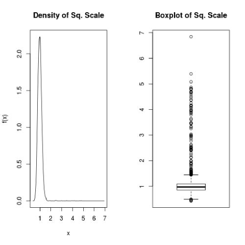
Figure 1: Density and simulation-based boxplot (n=10000) of the squared scaling variable, $V>0$, used for the example in this section. This scaling variable helps to construct fields that are very difficult to differentiate from Gaussian fields.

The behavior of scaling variable $V$ influences the tail behavior of the resulting vector $\mathbf{X}$. A typical representation of the multivariate Student distribution with correlation matrix $\Sigma$ and $\nu$ degrees of freedom is (see Kotz and Nadarajah [2004]):

$$\mathbf{X}=\sqrt{Q}\mathbf{Z}$$

where $\mathbf{Z}$ is a normally distributed vector with vector of means $\mathbf{0}$ and correlation matrix $\Sigma$, and

$$Q\sim\frac{\nu}{\chi_{\nu}^{2}}$$

Hence we can compare the distribution of squared scaling variable $V$, presented at figure 1 with the distribution of a multivariate Student distribution, for various degrees of freedom. The distributions of the squared scaling variables are presented at figure 2, for a multivariate Student distribution with $\nu\in\left\{10,15,20,35\right\}$ degrees of freedom.

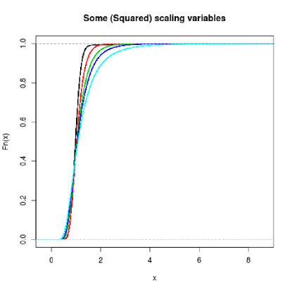
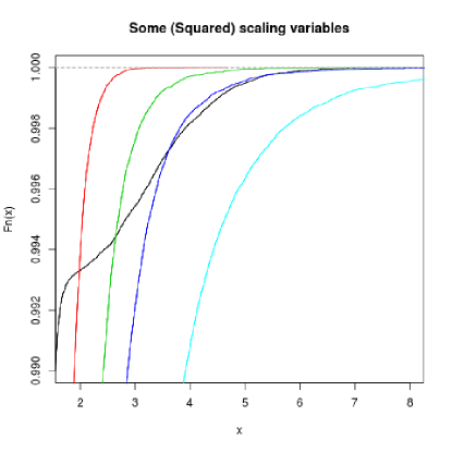
Figure 2: Comparison of the distribution of squared scaling variable $V$ (black) with distributions of the scaling variable of the multivariate Student distribution for degrees of freedom: 10 (light blue), 15 (dark blue), 20 (green), 35 (red). The uppermost part of the distribution of $V$ produces a tail behaviour similar to that of a multivariate Student distribution with 15 degrees of freedom.

It is noteworthy that scaling variable $V$ seems to have the lightest tail, if you focus on the left hand panel of figure 2. However, the uppermost part of the distribution of $V$ is similar to that of $\frac{\nu}{\chi_{\nu}^{2}}$ with $\nu=15$. That is, the tail dependence of our model is actually similar to that of the multivariate Student distribution with $\nu=15$ degrees of freedom. This fact goes completely unnoticed in the 1 and 2-dimensinal marginal distributions, as we shall show.

5.2 Partial observation of the fields: A network of 30 stations

Let us denote by $\mathbf{Z}^{*}\in\mathbb{R}^{J^{*}}$ and $\mathbf{X}^{*}\in\mathbb{R}^{J^{*}}$ the random fields generated as a Gaussian field, and by multiplication of the latter by $\sqrt{V}$, respectively. In this example, $J^{*}=300\times 300=90000$. We selected 30 components of the field, corresponding in a Spatial context to 30 locations on the plane, and stored the data of these components. The setting is illustrated in figure 3.

The n=3650, 30-dimensional observations thus available from field $\mathbf{Z}^{*}$ are in the following considered as realizations from sub-vector $\mathbf{Z}\in\mathbb{R}^{30}$ of $\mathbf{Z}^{*}$, whereas those from field $\mathbf{X}^{*}$ are considered as realizations of sub-vector $\mathbf{X}\in\mathbb{R}^{30}$.

Data from these vectors, $\mathbf{Z}$ and $\mathbf{X}$, represent the data available at a limited number of gauging stations. As usual in Spatial Statistics, we intend to identify characteristics of the whole fields, $\mathbf{Z}^{*}$ and $\mathbf{X}^{*}$, on the basis of the partial observations provided by $\mathbf{Z}$ and $\mathbf{X}$.

A third vector dealt with in this section is $\mathbf{W}\in\mathbb{R}^{30}$, of which each component is given by

$$W_{j}=F_{Z_{j}}^{-1}\left(F_{X_{j}}\left(X_{j}\right)\right)$$ (49)

that is, $\mathbf{W}$ is the vector resulting from applying the quantile-quantile transformation to each component of $\mathbf{X}$, mapping these into the quantiles of the components of $\mathbf{Z}$. Hence, each marginal distribution of $\mathbf{W}$ is exactly standard normal, like those of $\mathbf{Z}$, but the joint distribution of its ranks (the copula), is like that of $\mathbf{X}$.

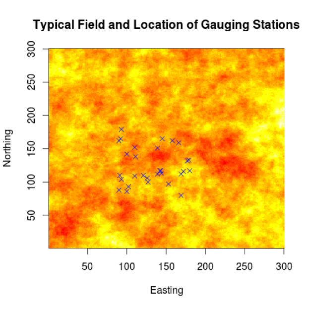
Figure 3: Typical (non-Gaussian) field of the n=3650 generated, and the 30 locations at which data was recorded to form $\mathbf{X}$ and $\mathbf{Z}$.

5.3 Invisibility of differences for standard Spatial Statistics diagnostics, and how to avoid this problem

A detailed analysis of the one and two dimensional marginal distributions (and copulas) of $\mathbf{X}$, $\mathbf{Z}$ and $\mathbf{W}$ on the basis of the data simulated is performed at C.

The analysis implies that all three random vectors can be modeled with a Gaussian distribution. In terms of current Spatial Statistics techniques, this means that the three fields, from which data collected are partial observations, can be safely modeled as a Gaussian field, with the same mean and covariance function parameters. This is of course wrong, but is all we can say if we just focus on one and two dimensional distributions.

In D, we present some aggregating statistics which can be employed to discriminate between the complete fields $\mathbf{X}^{*}\in\mathbb{R}^{90000}$ and $\mathbf{Z}^{*}\in\mathbb{R}^{90000}$, on the basis of the whole 30-dimensional data-sets available (not just its 2-dimensional marginals). We suggest that these statistics should be considered for model validation, in addition to statistics for one and two dimensional marginal distributions (including the covariance function). This will help to avoid missing important characteristics of data, which can have important implications for the inferred complete field, as seen in the following.

We have relegated these topics to the mentioned appendixes, in order to improve the readability of this paper.

5.4 Applications-relevant discrepancies in the underlying fields

The object of this section and of section (5.5) is to show what kind of inference about the complete fields can go wrong and unnoticed, if one does not pay attention to the discrepancies pointed out by the aggregating statistics shown in D. Please keep in mind that, according to the analysis of C, the three fields,$\mathbf{Z}^{*}$, $\mathbf{X}^{*}$ and $\mathbf{W}^{*}$, can be modeled by one and the same Gaussian model.

We focus on characteristics of the whole underlying fields, relevant for hydrological applications, in this section. In section 5.5 we deal with conditional distributions, more relevant for mining geostatistics.

We present two aggregating statistics of the complete fields, $\mathbf{Z}^{*}$, $\mathbf{X}^{*}$ and $\mathbf{W}^{*}$, portrayed in figure 3. We indicate the kind of global statistics that would go totally unnoticed, if we were to check only the one and two dimensional marginal distributions of the data available, and fit a Gaussian field for the whole geographical region.

Sums of positive values of the whole field

The first interaction manifestation we investigate is the distribution of

$$S_{\mathbf{X}^{*}}^{+}=\sum_{j=1}^{J=90000}\max\left(X_{j},0\right)$$ (50)

that is, the sum of positive values of the whole field, $\mathbf{X}^{*}$. Similarly, we define $S_{\mathbf{Z}^{*}}^{+}$ and $S_{\mathbf{W}^{*}}^{+}$ for fields $\mathbf{Z}^{*}$ and $\mathbf{W}^{*}$, respectively.

The distributions of the sums, $S_{\mathbf{X}^{*}}^{+}$, $S_{\mathbf{Z}^{*}}^{+}$ and $S_{\mathbf{W}^{*}}^{+}$, are investigated in terms of their sample quantiles. These are important statistics for rainfall modeling over a basin, for example, since a value proportional to this sum must find its way through the outlet of the basin, possibly causing a flood.

Boxplots illustrating the distribution of the sum of positive values are given in figure 4, whereas a table with some important sample quantiles of $S_{\mathbf{Z}^{*}}^{+}$, $S_{\mathbf{X}^{*}}^{+}$ and $S_{\mathbf{W}^{*}}^{+}$ are given in table 1. Notice that the sample quantiles of $S_{\mathbf{Z}^{*}}^{+}$ begin to deviate from those of $S_{\mathbf{X}^{*}}^{+}$ and $S_{\mathbf{W}^{*}}^{+}$ from the 99% quantile on. The relative percentage increase of the quantiles of $S_{\mathbf{X}^{*}}^{+}$ and $S_{\mathbf{W}^{*}}^{+}$ with respect to those of $S_{\mathbf{Z}^{*}}^{+}$ are given within parentheses in table 1.

Figure 4: Boxplots of sums of positive values for n realizations of $\mathbf{Z}^{*}$, $\mathbf{X}^{*}$ and $\mathbf{W}^{*}$, with $n=3650$.

Quantile	Gauss	Non-Gauss	Non-Gauss_QQ
80%	41901.96	41992.56 (+0.22%)	42288.41 (+0.92%)
90%	45342.97	46334.13 (+2.19%)	46576.23 (+2.72%)
95%	48609.21	49678.96 (+2.20%)	49910.30 (+2.68%)
99%	54906.90	57634.93 (+4.97%)	57583.49 (+4.87%)
99.5%	57660.03	62627.25 (+8.61%)	62794.43 (+8.90%)
99.9%	62331.09	81939.63 (+31.46%)	76972.03 (+23.49%)
100%	68099.17	100503.12 (+47.58%)	90353.53 (+32.68%)

Table 1: From left to right: Sample quantiles ($n=3650$) for $S_{\mathbf{Z}^{*}}^{+}$, $S_{\mathbf{X}^{*}}^{+}$ and $S_{\mathbf{W}^{*}}^{+}$. Percentages within parentheses indicate percentage increase with respect to data from the Gaussian field.

The sample size $n=3650$ would amount to a 10-year period, if data were to represent some daily measured variable. If the field $\mathbf{X}^{*}$ were to represent daily rainfall over a catchment, the maximum total rainfall would be 47.58% higher than one would expect by fitting a Gaussian model with adequate one and two dimensional marginal distributions and covariance function. By letting the simulation run up to $n=10000$ (roughly thirty years data), the increase in the maximum sum ascends to 61.11% for $\mathbf{X}^{*}$ and to $50.36\%$ for $\mathbf{W}^{*}$, as compared to the maximum sum produced by field $\mathbf{Z}^{*}$. These possibilities are completely missed by an analysis based on one and two dimensional marginal distributions, and the field’s covariance function.

Number of components of the whole field trespassing a given threshold

A second interaction manifestation we shall investigate for the complete fields, is the distribution of the number of components trespassing a given threshold. Analogously to (75), we define for $\mathbf{X}^{*}\in\mathbb{R}^{J^{*}}$,

$$L^{\mathbf{X}^{*}}=\sum_{j=1}^{J^{*}}1\left\{X_{j}^{*}>a\right\}$$

where $J^{*}=300\times 300$, and

$$1\left\{X_{j}^{*}>a\right\}=\begin{cases}1,&X_{j}^{*}>a\\ 0,&X_{j}^{*}\leq a\end{cases}$$ (51)

In the context of spatial statistics, $L^{\mathbf{X}^{*}}$ can be interpreted as the total area over which the environmental variable of interest realizes "extreme" values. Similar constructions define $L^{\mathbf{Z}^{*}}$ and $L^{\mathbf{W}^{*}}$. We have a total of $n=3650$ samples from each of these three random variables, which are plotted at figure 5 for thresholds 1.28 (left) and 2.5 (right).

Notice the great difference between the samples of $L^{\mathbf{Z}^{*}}$ and $L^{\mathbf{W}^{*}}$ (labeled "Gauss" and "Non-Gauss_QQ", respectively) when we use 2.5 as threshold. This occurs even though marginally fields $\mathbf{Z}^{*}$ and $\mathbf{W}^{*}$ have exactly the same distribution, and the covariance function of both fields is the same. In more practical terms, the difference in this variable amounts to $\mathbf{Z}^{*}$ and $\mathbf{W}^{*}$ having very different types of clusters of very high values, as illustrated in figure 6. Field $\mathbf{W}^{*}$ can exhibit much bigger clusters of values above 4 (99.99683% quantile of its marginal distribution), even though marginally and in terms of its covariance function it has the same specification as $\mathbf{Z}^{*}$.

Figure 5: Boxplots of the number of components above thresholds 1.28 (left) and 3.0 (right). The two non-gaussian fields are very different from the gaussian one with respect to this interaction manifestation. The difference is exacerbated as the threshold is pulled upwards. More extensive areas with very high values are to be expected for the non-gaussian fields.

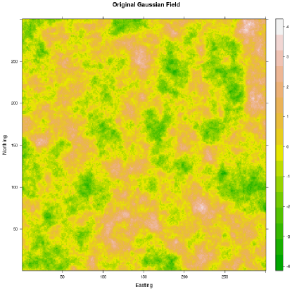
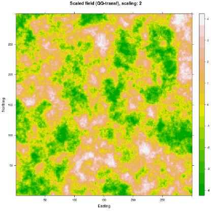
Figure 6: Different clustering characteristics between one realization of the gaussian (left) and non-gaussian (right) fields $\mathbf{Z}^{*}$ and $\mathbf{W}^{*}$. Scaling originally corresponding to non-gaussian field is $\sqrt{V}=2$. Field $\mathbf{W}^{*}$ can exhibit big clusters of values around 4, even though marginally and in terms of the covariance function it has the same specification as $\mathbf{Z}^{*}$.

5.5 Conditional distributions and interpolation

The conditional distribution of the random quantity at a new location, given a partial observation of the field will now be analyzed, by using the approximation given at equation (43). This is an important type of distribution in mining geostatistics, where inference on the random quantity investigated is necessary at unbored locations. We shall illustrate the type of discrepancy between the conditional distribution arising from a Gaussian model, as compared with that of the model given by equation (10). To this end, we focus on a realization of a sub-vector, $\mathbf{X}_{I}$, of $\mathbf{X}$. The set of indexes (i.e. locations) considered is $\left\{3,28,19,16,25,9,21\right\}$.

Vector

$$\mathbf{z}_{I}=\left(-1.489,-0.626,-0.050,0.068,0.491,0.832,-0.666\right)$$ (52)

constitutes the first realization of $\mathbf{Z}_{I}=\left(Z_{3},Z_{28},Z_{19},Z_{16},Z_{25},Z_{9},Z_{21}\right)$ of the random field shown at figure 6, left panel. Due to the mechanism depicted by equation (28), one can have immediately a realization, $\mathbf{x}_{I}$, of $\mathbf{X}_{I}=\left(X_{3},\ldots,X_{21}\right)$ by multiplying $\mathbf{Z}_{I}$ by probable values of scaling variable $\sqrt{V}$.

For our subsequent analysis we employ the following values as realizations of $\sqrt{V}$: 0.64, 1 and 2; hence obtaining three different realizations of $\mathbf{X}_{I}$. This will help us to understand why the two conditional fields of section 6 are so different: they correspond to a value of around $\sqrt{V}\approx\sqrt{6}$, as inferred from the data available.

We analyze the distribution of $Z_{3}$ and of $X_{3}$, conditioned on an increasing number of components of the vector. Such conditioning values are given by multiplying (52) times 0.64, 1 and 2. We plot percentiles: 80%, 90%, 95%, 99%, 99.5%, 99.9%, 99.99% and 99.999%.

In figure 7 we show the conditional distributions using $\sqrt{v}=0.64$ for $\mathbf{X}_{I}$. A moderate increase in the discrepancy between the conditional distributions is seen as the number of conditioning values increases, while the tail of the non-gaussian distribution becomes lighter and lighter as compared with that of the conditional Gaussian one.

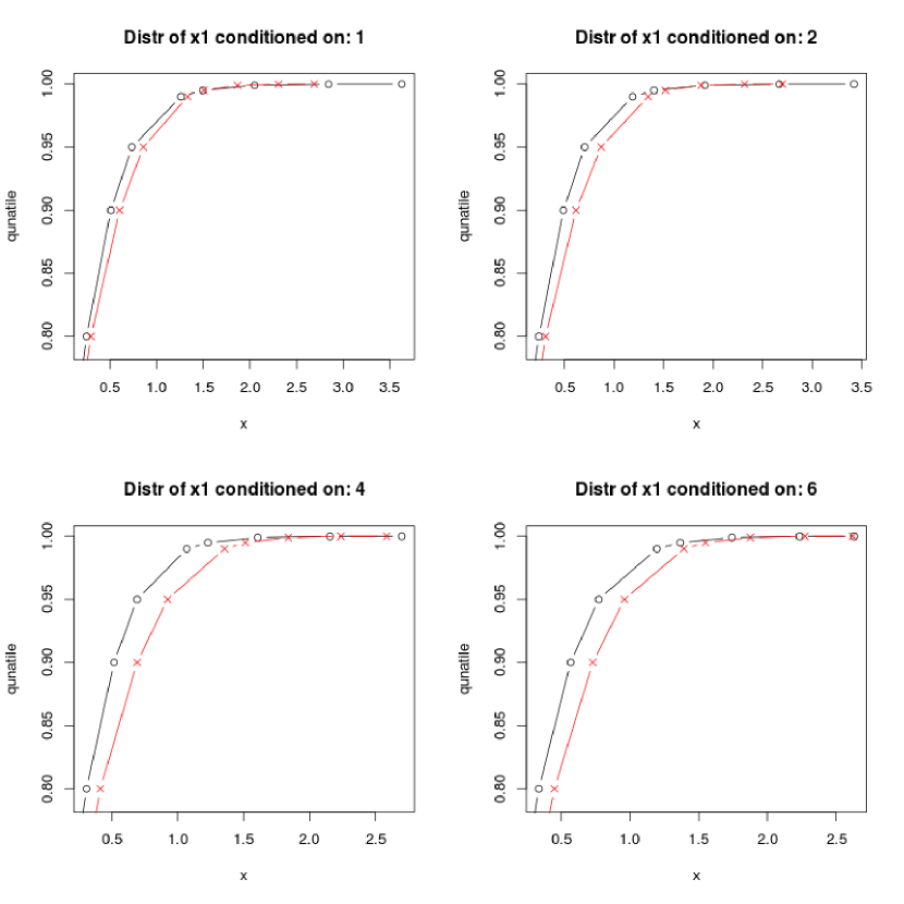
Figure 7: From left to right and downwards: Comparison of upper parts of conditional distributions for $Z_{3}$ (red) and $X_{3}$ (black), for $n=1,2,4,6$ conditioning values. Realization of $\mathbf{X}_{I}$ is given by $0.64\times\mathbf{z}_{I}$ (small scaling variable).

In figure 8 we show the conditional distributions using $\sqrt{v}=1$ for $\mathbf{X}_{I}$. Note that the non-gaussian conditional distribution keeps its similarity to the gaussian conditional, though it has higher quantiles for all conditioning schemes.

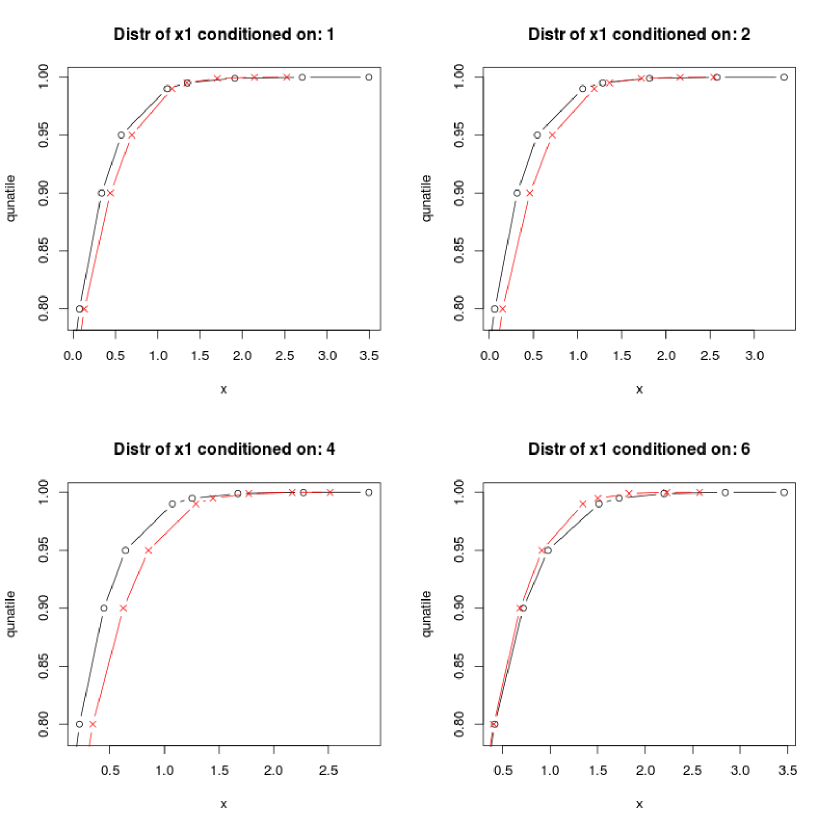
Figure 8: From left to right and downwards: Comparison of upper parts of conditional distributions for $Z_{3}$ (red) and $X_{3}$ (black), for $n=1,2,4,6$ conditioning values. Realization of $\mathbf{X}_{I}$ is given by $1\times\mathbf{z}_{I}$ (middle-valued scaling variable).

In figure 7 we show the conditional distributions using $\sqrt{v}=2$ for $\mathbf{X}_{I}$. The conditional distribution given one conditioning value is very similar for both models, but this situation quickly changes, as more conditioning values are considered. The quantiles of the upper part of the conditional distribution for $X_{3}$ become sensibly bigger already for 2 conditioning values. Note that the values one may expect for the conditioned ("ungauged") variable are considerably greater for $X_{3}$ than for $Z_{3}$. This is a relevant issue for applications.

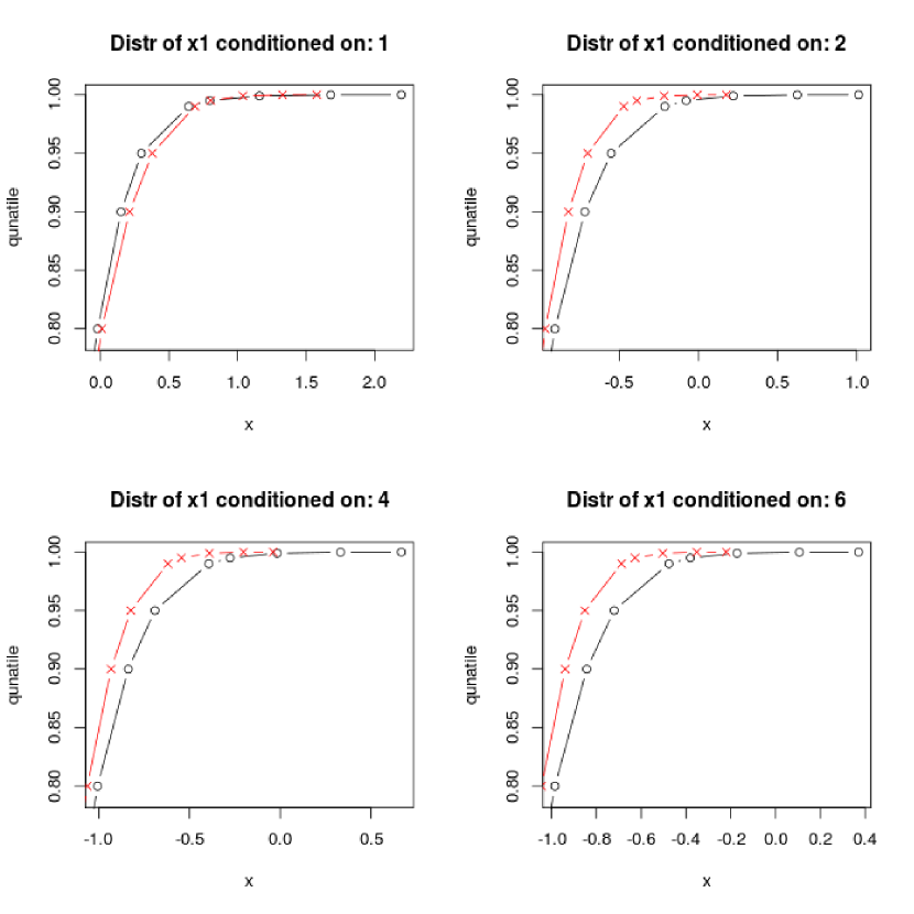
Figure 9: From left to right and downwards: Comparison of upper parts of conditional distributions for $Z_{3}$ (red) and $X_{3}$ (black), for $n=1,2,4,6$ conditioning values. Realization of $\mathbf{X}_{I}$ is given by $2\times\mathbf{z}_{I}$ (high-valued scaling variable).

5.6 Estimated parameters

We employ now the simple technique given in section 3.3 to estimate the additional parameters, $c_{2},\ldots,c_{5}$, corresponding to the cumulants of a non-degenerate (i.e. non-constant) scaling variable $V$. The estimated cumulants and moments of squared scaling variable $V$ are presented in table 2.

Using the method of moments, and the n=3650 data values, we fitted a mixture of 5 gamma distributions to each of the series of moments shown in table 2. The resulting distributions, together with the distribution of the original squared scaling variable $V>0$ are shown and compared in figure 10. The distribution of the scaling variable of a student multivariate distribution with 15 degrees of freedom, shown in blue, has been added for comparison.

Estimated	Gauss	Non-Gauss	Non-Gauss_QQ
m.1	1	1	1
m.2	0.9998	1.0792	1.0547
m.3	0.9988	1.4098	1.2378
m.4	0.9958	2.8072	1.8129
m.5	0.9897	9.0952	3.6831
c.1	1	1	1
c.2	-2e-04	0.0792	0.0547
c.3	-7e-04	0.1722	0.0738
c.4	-3e-04	0.6244	0.1806
c.5	2e-04	2.2289	0.4100

Table 2: Coefficients estimated by the method of moments, rounded up to four decimal places.

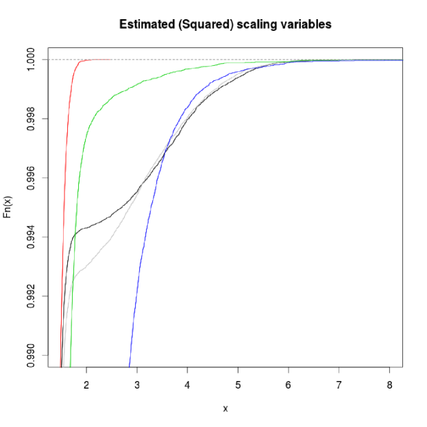
Figure 10: Estimated squared scaling variables, uppermost part: for $\mathbf{X}$ (black), $\mathbf{Z}$ (red), $\mathbf{W}$ (green), and a Student with 15 degrees of freedom (blue). The squared scaling variable originally employed for the simulation case study is shown in gray. The method of moments estimation was successful in capturing the uppermost behavior of the scaling variable.

We notice that the scaling variable is approximately recovered by this technique. However this technique cannot be used, for example, in the context of rainfall modeling, where data is constrained to be positive. Even though a latent variable approach (cf. Sansó and Guenni [1999]) can be employed for fitting the best Gaussian model to data (step 1 of estimation), the step effecting the estimation of additional parameters $c_{2},\ldots,c_{5}$ which determine important interaction manifestations of the field, cannot be executed via the method of moments: the latent imputed data correspond to a Normal distribution and hence does not produce valid realizations of squared generating variable, $R^{2}$.

A paper describing an alternative estimation method, which circumvents this difficulty, is already in preparation. For now, we present in a real context, that of the May-June of 2013 extreme rainfall over central Europe, what kind of inference may be unrealistic, if one validates one’s model only on the basis of one a two dimensional marginal distributions.

6 A glimpse at the June 2013 extreme central Europe rainfall events

We show in this section the implications of fitting a model that considers interactions beyond correlations, for modeling rainfall. We shall see that the probability of extreme rainfall over a whole catchment increases dramatically, even though, again, this is not noticed on the 1 and 2-dimensional marginal validation of the model. This has implications for forecasting and risk assessment.

At figure 11 we show a map of the Saalach river catchment, in southeast Germany. The catchment is relatively small, with an area of ca. 1043 $km^{2}$. Darker colors indicate higher elevations. The points plotted represent the locations of gauging stations recording total daily precipitation. The superimposed rectangle indicates the area to which our subsequent conditionally simulated fields refer.

We selected nine stations for our analysis, which are encircled in the map, since most of the stations are outside the catchment. However, these nine stations will suffice to make clear our argument about the need to consider multivariate interactions in Spatial Statistics modeling, for example, through the model we propose in this paper.

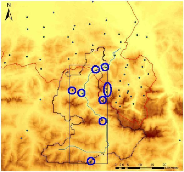
Figure 11: Catchment of the Saalach river. The rainfall gauging stations used for the analysis are shown encircled.

We fit to the daily data record from the 1st of January 2004 till the 31th of December 2009 a space-time model very similar to the one proposed by Sansó and Guenni [1999]. The following analysis constitutes by no means an attack on that model; we could have selected any other model which uses latent Gaussian fields, for example, that of Kleiber et al. [2012]. The model selected is convenient because it can easily accommodate missing data, of which we have some in our record. Estimation is performed in a Bayesian framework.

At the core of the model of Sansó and Guenni [1999] lies a latent Gaussian field, providing the spatial structure of the modeled rainfall field. We present in this section the implications of replacing this latent Gaussian field by a non-Gaussian one, built as in equation (28), but which is indistinguishable from a Gaussian field in its one a two dimensional marginals, as studied in the C.

On a given day, $t=1,\ldots,2192$, the data of the nine gauging stations are represented by vector $\mathbf{Y}_{t}=\left(Y_{t,1},\ldots,Y_{t,9}\right)$. We decompose the generic data vector into

$$\mathbf{Y}_{t}=\left(Y_{t,obs},Y_{t,zero},Y_{t,miss}\right)$$

where the components $Y_{t,obs}$, $Y_{t,zero}$ and $Y_{t,miss}$ represent the non-zero observed precipitation part, the no-precipitation observed part, and the missing part of vector $\mathbf{Y}_{t}$, respectively.

To avoid the problem posed by the vector parts $Y_{t,zero}$ and $Y_{t,miss}$, we use an “extended data” approach, whereby these parts are replaced by random vectors $W_{t}$ and $U_{t}$, respectively. All components of $W_{t}$ are constrained to be negative, whereas those of $U_{t}$ are not constrained.

Hence our typical data vector is given by

$$\mathbf{Y}_{t}=\left(Y_{t,obs},W_{t},U_{t}\right)$$

These vectors $W_{t}$ and $U_{t}$, for $t=1,\ldots,2192$, are then considered unknown parameters, and the posterior distributions found as part of the MCMC output.

Consider a time-evolving Gaussian field, $\mathbf{Z}_{t}$, connected to $\mathbf{Y}_{t}$ by the transformation $T^{-1}:\mathbf{Y}_{t}\rightarrow\mathbf{Z}_{t}$, with

$$\left(\begin{array}[]{c}Y_{t,obs}\\ W_{t}\\ U_{t}\end{array}\right)\underset{T^{-1}}{\rightarrow}\left(\begin{array}[]{c}Y_{t,obs}^{1/\beta_{m\left(t\right)}}\\ W_{t}\\ U_{t}\end{array}\right):=\mathbf{Z}_{t}$$ (53)

where $\beta_{m\left(t\right)}$ is a positive real number, and $m\left(t\right):t\rightarrow\left\{1,\ldots,12\right\}$ is a function mapping $t$ to its corresponding month of the year. Furthermore,

$$\mathbf{Z}_{t}\sim N_{9}\left(\mu_{t},\sigma_{m\left(t\right)}^{2}\Sigma\right)$$ (54)

where, for $j=1,\ldots,9$, we have

$$\mu_{t,j}=\alpha_{0}+\alpha_{1}h_{j}+\gamma_{m\left(t\right)}$$ (55)

with $h_{j}$ standing for elevation above sea level (i.e. an “external drift”) at the location of station $j$, and $\gamma_{m\left(t\right)}$ represents a monthly temporal effect. Function $m\left(t\right)$ is as before. This temporal effect is modeled by three harmonics,

$$\gamma_{m\left(t\right)}=\sum_{r=1}^{3}\left\{A_{r}\cos\left(\frac{2\pi r}{12}m\left(t\right)\right)+B_{r}\sin\left(\frac{2\pi r}{12}m\left(t\right)\right)\right\}$$ (56)

to allow for variability within the year’s cycle.

Correlation matrix, $\Sigma\in\mathbb{R}^{9\times 9}$, is assumed to follow an exponential correlation function,

$$\Sigma_{j_{1},j_{2}}=\exp\left(-\lambda\left\|\mathbf{s}_{j_{1}}-\mathbf{s}_{j_{2}}\right\|\right)$$ (57)

where $\lambda>0$ is an unknown scale parameter, $\mathbf{s}_{j_{1}}$ and $\mathbf{s}_{j_{2}}$ stand for the locations on $\mathbb{R}^{2}$ of stations $j_{1}$ and $j_{2}$, and the symbol $\left\|*\right\|$ represents the Euclidean distance. The (spatially) common variance $\sigma_{m\left(t\right)}^{2}$ is allowed to change with the month on which $t$ falls.

We assume flat prior distributions on all parameters, and a priori independence among the parameters, so that

$$p\left(\alpha_{0},\alpha_{1},A_{1},\ldots,B_{3},\lambda,\sigma_{1}^{2},\ldots,\sigma_{12}^{2},W_{1},\ldots,U_{2192}\right)\propto 1_{\left\{\lambda>0,W_{t}<0\right\}}$$ (58)

where $1_{\left\{A\right\}}$ is the indicator variable for the event $\left\{A\right\}$. We refer to all parameters collectively as $\Phi$.

That the issues of zero valued observations and missing data have been conveniently solved, can be seen from the relative simplicity of the resulting likelihood function of the extended data, on which our inference is based. Defining $J_{t}$ as the set of indexes of $Y_{t,obs}$ for each $t=1,\ldots,2192:=T$, one has:

$$L_{data}\left(\Phi\right)\propto\frac{\prod_{t=1}^{T}\left(\prod_{J_{t}}\frac{1}{\beta_{m\left(t\right)}}y_{j\in J_{t}}^{\frac{1}{\beta_{m\left(t\right)}}-1}\right)}{\left(\prod_{t=1}^{T}\left(\sigma_{m\left(t\right)}^{2}\right)^{\frac{J}{2}}\right)\left|\Sigma\right|^{\frac{T}{2}}}\times\\ \exp\left(-\frac{1}{2}\sum_{t=1}^{T}\left\{\frac{1}{\sigma_{m\left(t\right)}^{2}}\left(T^{-1}\left(\mathbf{y}_{t}\right)-\mu_{t}\right)^{{}^{\prime}}\Sigma^{-1}\left(T^{-1}\left(\mathbf{y}_{t}\right)-\mu_{t}\right)\right\}\right)$$ (59)

For example, no integration is required for (59). We refer the reader to Sansó and Guenni [1999] for details on this type of model.

For our purposes, it suffices to present here the estimated parameters, computed as the mean values of the respective Markov Chains, after letting sufficiently many burn-in iterations of the Metropolis Hastings algorithm run (11000, in our case). The estimates are given on table 3, rounded up to the fourth decimal place.

$\alpha_{i}$,$i=0,1$	$\beta_{i}$, $i=1,\ldots,12$	$\sigma_{i}^{2}$, $i=1,\ldots,12$	$A_{i}$, $i=1,2,3$	$B_{i}$, $i=1,2,3$	$\lambda$
-0.0644	1.8503	15.5086	-0.8199	-0.0214	0.0221
0.0001	1.6930	13.1596	0.3916	0.4156
	1.8016	11.1473	-0.1907	-0.3885
	1.7018	14.0445
	1.6415	18.7905
	1.5893	15.1922
	1.4565	31.2774
	1.6544	22.8418
	1.7055	20.4347
	1.5693	11.5969
	1.6610	20.4527
	1.6910	10.0384

Table 3: Parameters fitted for the Space-Time model. The indexes “i” increase downwards.

As mentioned earlier, we are currently working on a coherent estimation method for estimating all parameters simultaneously. For the moment, in order to show the implications of considering higher order interdependences, we multiply the latent Gaussian field fitted using the MCMC method times the scaling variable of section (5.1). Thereby we obtain a latent field of the form (28). Note that, according to the analysis of C, these two latent fields are not distinguishable by analyzing their one and two dimensional marginal distributions.

The rectangle superimposed on figure 11 is formed of a $33\times 83$ grid, in which each square side represents a 500 meter length. Using the fitted parameters of table 3, we obtain the mean value $\mu_{t,j}$ at each location $j=1,\ldots,2739$, and we get also the correlation matrix for the whole $33\times 83$ grid.

We then simulated for each month of the year 3000 realizations, $\mathbf{z}_{t}\in\mathbb{R}^{2739}$, of the latent Gaussian field using the parameters extended to the $33\times 83$ grid. We set the negative values of these Gaussian vectors to zero, and ten applied the transformation $\mathbf{z}_{t}\rightarrow\mathbf{z}_{t}^{\beta_{m\left(t\right)}}:=\mathbf{y}_{t}$. Vectors $\mathbf{y}_{t}$ are our simulated precipitations fields with latent Gaussian structure.

To obtain vectors $\tilde{\mathbf{y}_{t}}$ which consider interdependence beyond correlation, we simulated $3000\times 12=36000$ realizations, $v_{t}$, of the scaling variable $V$ from section 5.1, 3000 for each month of the year. We set $\tilde{\mathbf{z}}_{t}=\mu_{t}+\left(\mathbf{z}_{t}-\mu_{t}\right)\times\sqrt{v_{t}}$ ; the negative components of these vectors were set to zero, and then we applied the transformation $\tilde{\mathbf{z}}_{t}\rightarrow\tilde{\mathbf{z}}_{t}^{\beta_{m\left(t\right)}}:=\tilde{\mathbf{y}}_{t}$. Vectors $\tilde{\mathbf{y}}_{t}$ are our simulated precipitation fields with latent non-Gaussian structure.

By averaging the values of the components of vectors $\mathbf{y}_{t}$ and $\tilde{\mathbf{y}}_{t}$, we get for each type of field 3000 average precipitation values per month, over the rectangular area shown at figure 11. These values are plotted in figure 12. Note that the distribution of the average values of both fields is very similar, except that some values of the field with non-Gaussian latent structure are much bigger than those expectable from a model with latent Gaussian structure. This is the effect of interactions among more than two variables.

Is these simulations were to be included as forecasts in a model for flood risk assessment, for example, the forecast based on the space-time model with Gaussian latent structure would suggest much longer flood return periods.

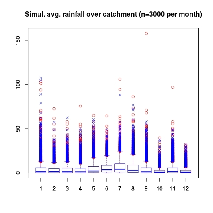
Figure 12: Boxplots of the 3000 per month unconditional simulations from the field with latent Gaussian structure (blue), and the field with non-Gaussian latent structure (red). Values are in millimeters. The interaction of order greater than two among components can trigger very high simultaneous values in the components of the random field.

The entropy-based graphical technique of D can be used for validation of the model with Gaussian latent structure. We focus on the three stations having less missing values, out of the 9 stations (labeled 1,2 and 3 in figure 15).

In figure 13, the graphical validation tool is presented for thresholds $a\in\left\{.80,.85,.90,.95,.99,.995\right\}$. The 3-wise observed association is considerably bigger, up to a threshold of 0.95. A simulation-based 90% confidence interval is also shown. This is an indicator that the model is systematically underestimating 3-wise association. Note that this technique is robust to non-decreasing transformations on the marginal distributions.

We are currently working on techniques to systematically estimate scaling variable, $V$, of the latent non-Gaussian field, such that the resulting 3-wise association is more similar to the observed one.

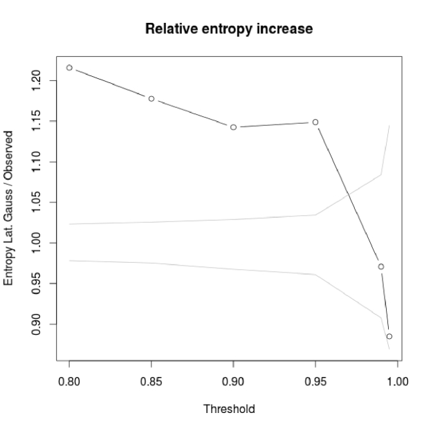
Figure 13: Ratio of congregation measures and 90% confidence interval, as explained in D, for the three stations labeled 1, 2 and 3. Three-wise association of data is considerable higher up to threshold 0.95.

6.1 Conditional simulation for the 1st of June 2013

Although our model was fitted with data from 2004-2009, we now show that the probability of very intense precipitations, such as those of early June 2013 over the Saalach river catchment, can be more realistically evaluated if we consider higher order interactions in our space-time model.

Taking a close look at the available data of the nine stations selected, one finds very high values at virtually all stations for June the 1st 2013. The next day, June the 2nd, there was a tremendous increase in the water flow of river Saalach, according to discharge measurements at the village of Unterjettenberg, very near to the town of Bad Reichenhall, in southeast Germany.

Hence in this section we produce rainfall fields, conditional on the observed data of June 1st 2013, for the rectangular area presented in figure 11. This is a good proxi for the average precipitation over the whole Saalach catchment. To produce the conditional simulations, we used the second technique presented at section 4.2.

Only four gauging stations have data for June 1st 2013. These stations are shown in red in figure 15; we shall address this figure shortly. The four stations with observed data are also labeled 1,2,3 and 4, in the figure. Their data values (in mm) are: 104.1, 120.0, 85.1 and 65.1, respectively.

The first step in generating the conditional fields, according to the technique in section 4.2, is to obtain a sample of the scaling variable, $V$, conditional on the observed data. The sampled scaling variable is shown at figure 14. Note the high values for $V$ (up to $V=10$) that are consistent with the observed high rainfall values.

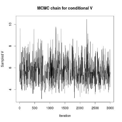
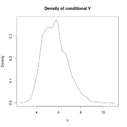
Figure 14: Sampled scaling variable, $V$, for June 1st 2013, conditional on observed values: MCMC chain after 500 burn-in iterations (left), and estimated probability density (right).

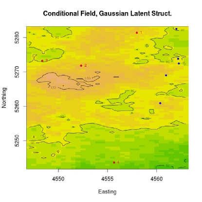
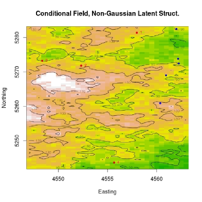
Figure 15: Two conditionally simulated fields for June 1st 2013: Field with Gaussian latent structure (left), and field with non-Gaussian latent structure (right). Stations providing the observed data are indicated in red.

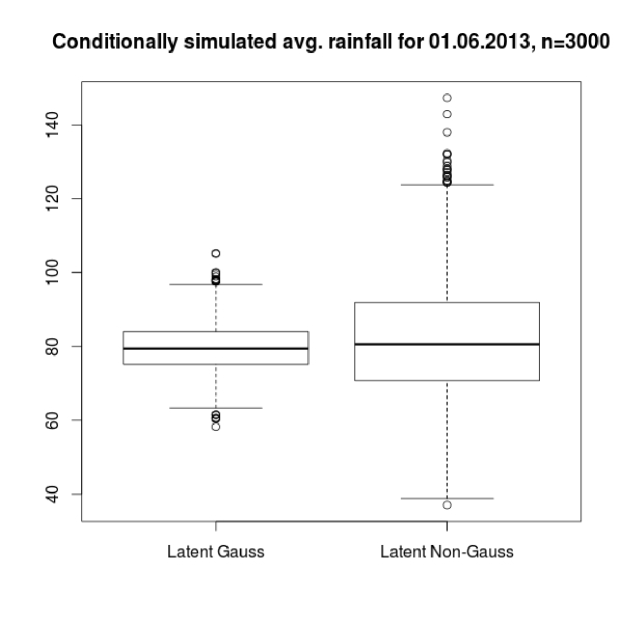
Figure 16: Boxplots of the average of the conditionally simulated random fields for June 1st 2013, in millimeters. The field with high oder interacting latent structure shows much more variability. In particular, average precipitation over the catchment above 120 mm are quite probable under the new model.

Using these sampled $V$’s, we generated the conditional fields, 3000 in total. Two realizations of these fields are presented in figure 15. The contrast between them is by no means atypical.

Note the two intense clusters, with values of over 170 mm each, which one encounters in the realization of the field with multivariate interactions (right panel). On the other hand, other regions of the map exhibit lower values than the field with the Gaussian latent structure; for example, the southeast region has slightly smaller values.

Using the 3000 conditional simulations for each field, we have an idea of the kind extreme event we can expect over the catchment, according to each of the models. We focus on the mean catchment precipitation, as before. In figure 16 we show boxplots of the average of the simulated fields. Note that values above 120 mm seem quite probable for the model with non-Gaussian latent structure, whereas they seem to be almost improbable for the model with Gaussian latent structure.

Whether the true average rainfall over the Saalach river catchment was 120 mm or more on June 1st 2013, is not yet clear; that statement would require a detailed analysis of the river discharge, and of the meteorological conditions during the days immediately before, and up to that day. But with this example we hope at least to show the need to develop models that consider explicitly interactions among groups of variables. Such interactions have the potential, as we have seen, to increase greatly the probability of very high values at several locations simultaneously.

Considering these interactions might lead to more realistic estimated flood return periods for the towns in the catchment which lie near the river.

7 Discussion and work in progress

The model introduced by (10) allows for the explicit consideration of joint cumulants of order greater than two (i.e. not just covariances) in a manner that is convenient for spatial modeling: building on available geostatistical techniques, requiring a minimum of extra parameters, and respecting the principle of spatial consistency. The range of tail dependence intensity of this model goes from zero (i.e. Gaussian) to that of a Student-t, as in the synthetic example presented.

The need in Spatial Statistics to consider interactions among more than two variables at a time was illustrated using a thorough synthetic case study. We also analyzed the possible implications of high order interdependence for the forecasting of the total volume of precipitation over the Saalach river catchment, in Germany.

The presence of interactions, not noticeable from the one and two dimensional marginals, can be assessed using statistics that aggregate information of higher dimensional marginal distributions of the data. We presented some of such statistics. To make sure that data simulated from the model reproduces those statistics (i.e. those interaction manifestations) is an important complementary goodness of fit procedure for a spatial model.

This paper has provided the theoretical basis for a model with which interactions among more than two variables can be explicitly considered. But there is much work to do in order to exploit the full power of the model. A parameter estimation procedure more convenient than the one presented here, usable also for truncated data (e.g. for precipitation modeling) is under development. We also intend to connect the scaling variable used to build our model, and which determines the additional interaction characteristics, with large scale atmospheric processes, in a hierarchical manner. In this way we expect to produce more realistic forecasts of intense precipitation over large areas, for the sake of risk assessment.

Acknowledgments

This research forms part of the Ph.D thesis of the first author, which was funded by a scholarship of the German Academic Exchange Service (DAAD), and realized in the context of the ENWAT program of the University of Stuttgart.

We also thank Prof. Lelys Bravo de Guenni for her critical review of this work and her very useful comments. The responsibility for any mistake in the text is of course entirely of the authors.

Appendix A Derivation of joint cumulants of the model

Our object of study is the cumulant generating function of a random variable $\mathbf{X}\in\mathbb{R}^{J}$. We shall be interested in joint cumulants such as

$$cum\left(X_{j_{1}},\ldots,X_{j_{r}}\right)$$ (60)

where some, or all, of the indexes can be repeated. Hence it is convenient to refer to a random vector $\mathbf{X^{*}}\in\mathbb{R}^{J^{*}}$ having the components of $\mathbf{X}$, even repeated, and then find the joint cumulants that appear with degree at most one, of this “new” random vector. Thus we can, without loss of generality, focus on finding the joint cumulants with degree not greater than one, given by

$$\frac{\partial^{r}}{\partial t_{j_{r}}\ldots\partial t_{j_{1}}}K_{\mathbf{X^{*}}}\left(\mathbf{t}\right)\mid_{\mathbf{t}=\mathbf{0}}:=cum\left(X_{j_{1}},\ldots,X_{j_{r}}\right)$$ (61)

where no $t_{j}$, for $j\in\left\{j_{1},\ldots,j_{r}\right\}$, is repeated.

For example, when computing the variance of a component, $X_{j}$, of $\mathbf{X}$, one would rather compute the covariance of vector $\mathbf{X}^{*}=\left(X_{j},X_{j}\right)$, namely $\kappa_{11}\left(\mathbf{X^{*}}\right)$.

The archetypal dependence structure advocated for in this work is given by

$$K_{\mathbf{X^{*}}}\left(\mathbf{t}\right)=c_{1}\frac{1}{2}\mathbf{t^{T}\Gamma t}+\frac{1}{2!}c_{2}\left[\frac{1}{2}\mathbf{t^{T}\Gamma t}\right]^{2}+\frac{1}{3!}c_{3}\left[\frac{1}{2}\mathbf{t^{T}\Gamma t}\right]^{3}+\ldots$$ (62)

for some coefficients $c_{1},c_{2},c_{3},\ldots$ and covariance matrix $\Gamma_{J^{*}\times J^{*}}$, and $\mathbf{t}\in\mathbb{R}^{J^{*}}$.

By expansion, the above expression can be written as

$$K_{\mathbf{X^{*}}}\left(\mathbf{t}\right)=\frac{c_{1}}{1!}\frac{1}{2}\sum_{j_{1},j_{2}=1}^{J}t_{j_{1}}t_{j_{2}}\Gamma_{j_{1}j_{2}}+\frac{c_{2}}{2!}\frac{1}{2^{2}}\sum_{j_{1},\ldots,j_{4}=1}^{J}t_{j_{1}}\ldots t_{j_{4}}\Gamma_{j_{1}j_{2}}\Gamma_{j_{3}j_{4}}+\\ \frac{c_{3}}{3!}\frac{1}{2^{3}}\sum_{j_{1},\ldots,j_{6}=1}^{J}t_{j_{1}}\ldots t_{j_{6}}\Gamma_{j_{1}j_{2}}\Gamma_{j_{3}j_{4}}\Gamma_{j_{5}j_{6}}+\ldots$$ (63)

For each coefficient $c_{\frac{r}{2}}$, for $r$ even, there appears a sum of the form

$$\frac{c_{\frac{r}{2}}}{\frac{r}{2}!}\frac{1}{2^{\frac{r}{2}}}\sum_{j_{1}=1}^{J}\ldots\sum_{j_{2r}=1}^{J}t_{j_{1}}\ldots t_{j_{r}}\Gamma_{j_{1}j_{2}}\ldots\Gamma_{j_{r-1}j_{r}}$$ (64)

This is the only block-summand of (63) that does not vanish upon differentiation with respect to each variable and equation to zero, as in (61). Other blocks will vanish either upon differentiation with respect to a variable that does not appear in them, or upon equation to zero, since such blocks become a sum of zeroes. So, it suffices to focus on this block, to differentiate it and equate it with zero.

Let each member of the (64) be labeled

$$s_{j_{1}\ldots,j_{r}}=t_{j_{1}}\ldots t_{j_{r}}\Gamma_{j_{1}j_{2}}\ldots\Gamma_{j_{r-1}j_{r}}$$

then, we have stated that,

$$\frac{\partial^{r}}{\partial t_{j_{r}}\ldots\partial t_{j_{1}}}K_{\mathbf{X^{*}}}\left(\mathbf{t}\right)\mid_{\mathbf{t}=\mathbf{0}}=\frac{c_{\frac{r}{2}}}{\frac{r}{2}!}\frac{1}{2^{\frac{r}{2}}}\sum_{j_{1}=1}^{J}\ldots\sum_{j_{2r}=1}^{J}\frac{\partial^{r}}{\partial t_{j_{r}}\ldots\partial t_{j_{1}}}s_{j_{1},\ldots,j_{r}}$$ (65)

Partial differentiation of $s_{j_{1},\ldots,j_{r}}$ is readily found to be

$$\frac{\partial^{r}}{\partial t_{j_{r}}\ldots\partial t_{j_{1}}}s_{j_{1},\ldots,j_{r}}=\Gamma_{j_{1}j_{2}}\ldots\Gamma_{j_{r-1}j_{r}}$$ (66)

Sub-indexes appearing in the factors, $\Gamma_{j_{1}j_{2}}$, $\Gamma_{j_{3}j_{4}},\ldots$ constitute a partition of size $\frac{r}{2}$ of the set $A=\left\{j_{1},j_{2},\ldots,j_{r}\right\}$. That is, the union of the $\frac{r}{2}$ non-overlapping sets

$$\left\{j_{1},j_{2}\right\},\left\{j_{3},j_{4}\right\},\ldots,\left\{j_{r-1},j_{r}\right\}$$

formed with elements of set $A=\left\{j_{1},j_{2},\ldots,j_{r}\right\}$, is equal to that set:

$$\left\{j_{1},j_{2}\right\}\cup\left\{j_{3},j_{4}\right\}\cup\ldots\cup\left\{j_{r-1},j_{r}\right\}=A$$

Since the sum at (65) runs over all indexes in $A$, the sum returning the joint cumulant in question comprises all partitions of size two of $A$. How many different partitions of size two can be obtained for $A$, by forming sets out of different combinations of indexes? In general, a set with $n$ elements, $n$ even, can be seen to have

$$1\times 3\times\ldots\times\left(n-1\right)$$

such partitions.

We have shown that joint cumulants of the archetypal dependence structure are given by

$$cum\left(X_{j_{1}},\ldots,X_{j_{r}}\right)=\frac{c_{\frac{r}{2}}}{\frac{r}{2}!}\frac{1}{2^{\frac{r}{2}}}\sum_{j_{1},\ldots,j_{r}=1}^{J}\Gamma_{j_{1}j_{2}}\ldots\Gamma_{j_{r-1}j_{r}}$$ (67)

Appendix B Relation between moments of squared scaling variable and generating variable

Assume that we have random vector $\mathbf{Z}\in\mathbb{R}^{J}$ with c.g.f (10), with $\mathbf{\mu}=\mathbf{0}$ and covariance matrix equal to the identity matrix, $\Sigma=I_{J\times J}$. For this special case, in agreement with representation (5), we have

$$\left\|\mathbf{Z}\right\|_{2}=\sqrt{\left\|\mathbf{Z}\right\|_{2}\left\|\mathbf{Z}\right\|_{2}}=\sqrt{\left\|R\times\mathbf{U}^{J-1}\right\|_{2}\left\|R\times\mathbf{U}^{J-1}\right\|_{2}}=R\times 1$$

since $\left\|\mathbf{U}^{J-1}\right\|_{2}=1$. Then,

$$R^{2}=\sum_{j=1}^{J}Z_{j}^{2}$$ (68)

which in turn means that,

$$E\left(\left(R^{2}\right)^{k}\right)=E\left(\left(\sum_{j_{1}=1}^{J}Z_{j_{1}}^{2}\right)\times\ldots\times\left(\sum_{j_{k}=1}^{J}Z_{j_{k}}^{2}\right)\right)=\sum_{j_{1}=1}^{J}\ldots\sum_{j_{k}=1}^{J}E\left(Z_{j_{1}}^{2}\ldots Z_{j_{k}}^{2}\right)$$ (69)

Since $\mathbf{Z}$ has c.g.f. given by

$$K_{\mathbf{Z}}\left(\mathbf{t}\right)=\frac{c_{1}}{1!}\left(\frac{1}{2}\mathbf{t^{{}^{\prime}}t}\right)+\frac{c_{2}}{2!}\left(\frac{1}{2}\mathbf{t^{{}^{\prime}}t}\right)^{2}+\frac{c_{3}}{3!}\left(\frac{1}{2}\mathbf{t^{{}^{\prime}}t}\right)^{3}+\ldots$$

it follows, as seen in section 2, that

$$M_{\mathbf{Z}}\left(\mathbf{t}\right)=1+\frac{m_{1}}{1!}\left(\frac{1}{2}\mathbf{t^{{}^{\prime}}t}\right)+\frac{m_{2}}{2!}\left(\frac{1}{2}\mathbf{t^{{}^{\prime}}t}\right)^{2}+\frac{m_{3}}{3!}\left(\frac{1}{2}\mathbf{t^{{}^{\prime}}t}\right)^{3}+\ldots$$

with coefficients given by

$$m_{1} = c_{1}$$

$$m_{2} = c_{2}+c_{1}^{2}$$

$$m_{3} = c_{3}+3c_{2}c_{1}+c_{1}^{3}$$

$$m_{4} = c_{4}+4c_{3}c_{1}+3c_{2}^{2}+6c_{2}c_{1}^{2}+c_{1}^{4}$$ (70)

and so on. A particular case of this function is the Gaussian moment generating function, for which all $c_{r>1}$ are set to zero. In particular, for $\xi\sim N_{J}\left(\mathbf{0},I_{J\times J}\right)$,

$$M_{\mathbf{\xi}}\left(\mathbf{t}\right)=1+\frac{c_{1}}{1!}\left(\frac{1}{2}\mathbf{t^{{}^{\prime}}t}\right)+\frac{c_{1}^{2}}{2!}\left(\frac{1}{2}\mathbf{t^{{}^{\prime}}t}\right)^{2}+\frac{c_{1}^{3}}{3!}\left(\frac{1}{2}\mathbf{t^{{}^{\prime}}t}\right)^{3}+\ldots$$ (71)

with $c_{1}=1$. Hence joint moments of $\mathbf{Z}$ and $\mathbf{\xi}$ are similar, except for what pertains to coefficients $c_{2},c_{3},\ldots$. In fact, calling

$$h_{r}\left(\mathbf{t}\right)=\left(\frac{1}{2}\mathbf{t^{{}^{\prime}}t}\right)^{r}$$

one has

$$\begin{cases}\frac{\partial^{r_{1}+\ldots+r_{k}}}{\partial t_{j_{1}}\ldots\partial t_{j_{k}}}M_{\mathbf{\xi}}\left(\mathbf{t}\right)=\frac{c_{1}}{1!}\frac{\partial^{r_{1}+\ldots+r_{k}}}{\partial t_{j_{1}}\ldots\partial t_{j_{k}}}h_{1}\left(\mathbf{t}\right)+\frac{c_{1}^{2}}{2!}\frac{\partial^{r_{1}+\ldots+r_{k}}}{\partial t_{j_{1}}\ldots\partial t_{j_{k}}}h_{2}\left(\mathbf{t}\right)+\ldots\\ \frac{\partial^{r_{1}+\ldots+r_{k}}}{\partial t_{j_{1}}\ldots\partial t_{j_{k}}}M_{\mathbf{Z}}\left(\mathbf{t}\right)=\frac{m_{1}}{1!}\frac{\partial^{r_{1}+\ldots+r_{k}}}{\partial t_{j_{1}}\ldots\partial t_{j_{k}}}h_{1}\left(\mathbf{t}\right)+\frac{m_{2}}{2!}\frac{\partial^{r_{1}+\ldots+r_{k}}}{\partial t_{j_{1}}\ldots\partial t_{j_{k}}}h_{2}\left(\mathbf{t}\right)+\ldots\end{cases}$$

Hence, for odd orders joint moments of both random vectors are zero, and for even orders

$$E\left(\xi_{i}\xi_{j}\right) = \frac{c_{1}}{m_{1}}E\left(Z_{i}Z_{j}\right)$$

$$E\left(\xi_{i}\xi_{j}\xi_{k}\xi_{l}\right) = \frac{c_{1}^{2}}{m_{2}}E\left(Z_{i}Z_{j}Z_{k}Z_{l}\right)$$

$$\vdots$$

$$E\left(\xi_{j_{1}}^{r_{1}}\ldots\xi_{j_{k}}^{r_{k}}\right) = \frac{c_{1}^{\frac{1}{2}\sum_{j=1}^{k}r_{j}}}{m_{\frac{1}{2}\sum_{j=1}^{k}r_{j}}}E\left(Z_{j_{1}}^{r_{1}}\ldots Z_{j_{k}}^{r_{k}}\right)$$

whenever $order=\sum_{i=1}^{k}r_{i}$ is an even integer. It is then clear that the following relation holds, for joint moments of even order:

$$\frac{m_{1}}{c_{1}}E\left(\xi_{i}\xi_{j}\right) = E\left(Z_{i}Z_{j}\right)$$

$$\frac{m_{2}}{c_{1}^{2}}E\left(\xi_{i}\xi_{j}\xi_{k}\xi_{l}\right) = E\left(Z_{i}Z_{j}Z_{k}Z_{l}\right)$$

$$\vdots$$

$$\frac{m_{\frac{1}{2}\sum_{j=1}^{k}r_{j}}}{c_{1}^{\frac{1}{2}\sum_{j=1}^{k}r_{j}}}E\left(\xi_{j_{1}}^{r_{1}}\ldots\xi_{j_{k}}^{r_{k}}\right) = E\left(Z_{j_{1}}^{r_{1}}\ldots Z_{j_{k}}^{r_{k}}\right)$$ (72)

Product moments appearing on the left hand side of equation (72) can be readily found, since they are the moments of a multivariate Gaussian distribution with covariance matrix equal to identity matrix $I_{J\times J}$.

Coefficients $m_{1},m_{2},m_{3},\ldots$ are given in terms of $c_{1},c_{2},c_{3},\ldots$ (and vice versa). Hence we have, by virtue of (69), identified requirements on all moments of (squared) generating variable $R^{2}$, so that the resulting multivariate distribution $\mathbf{X}$ has cumulant generating function (10).

Summarizing these results:

First, since the multivariate Gaussian distribution referred to at equation 72 has covariance matrix equal to identity, one can write for any set of components $\left(j_{1},\ldots,j_{k}\right)$,

$$\frac{m_{k}}{c_{1}^{k}}E\left(\xi_{j_{1}}^{2}\ldots\xi_{j_{k}}^{2}\right)=E\left(Z_{j_{1}}^{2}\ldots Z_{j_{k}}^{2}\right)$$ (73)

where $\xi$ is a $J$-dimensional normally distributed vector with mean vector $\mathbf{0}$ and covariance matrix $I_{J\times J}$, the identity matrix on $\mathbb{R}^{J\times J}$. Equation (69) holds in particular for vector $\xi$, in which case $R^{2}\sim\chi_{J}^{2}$, and

$$\sum_{j_{1}=1}^{J}\ldots\sum_{j_{k}=1}^{J}E\left(\xi_{j_{1}}^{2}\ldots\xi_{j_{k}}^{2}\right)=E\left(\left(\chi_{J}^{2}\right)^{k}\right)=\frac{2^{k}\Gamma\left(k+\frac{J}{2}\right)}{\Gamma\left(\frac{J}{2}\right)}$$

Second and more importantly, by virtue of (73), one can re-write (69) as

$$E\left(\left(R^{2}\right)^{k}\right)=\sum_{j_{1}=1}^{J}\ldots\sum_{j_{k}=1}^{J}\frac{m_{k}}{c_{1}^{k}}E\left(\xi_{j_{1}}^{2}\ldots\xi_{j_{k}}^{2}\right)=\frac{m_{k}}{c_{1}^{k}}\frac{2^{k}\Gamma\left(k+\frac{J}{2}\right)}{\Gamma\left(\frac{J}{2}\right)}$$ (74)

which expresses the moments of $R^{2}$ in terms of parameters $m_{k}$ (hence indirectly of $c_{k}$) and the dimension of the random vector $\mathbf{X}$.

Appendix C Similarity of one and two dimensional marginal distributions

In this section, we show that the one and two dimensional marginal distributions of the data collected from random vectors $\mathbf{X}\in\mathbb{R}^{30}$, $\mathbf{W}\in\mathbb{R}^{30}$ and $\mathbf{Z}\in\mathbb{R}^{30}$ at section 5 are practically indistinguishable. They all seem to be Guassian random vectors.

C.1 Analysis of one dimensional marginal distributions

Comparison of the 1-dimensional marginal distributions of $\mathbf{Z}$ and $\mathbf{X}$ is performed in this sub-section. At figure 17 we present four quantile-quantile plots. Each of these plots corresponds to data from $\left(Z_{j},X_{j}\right)$, where $j$ has been randomly selected from $\left\{1,\ldots,30\right\}$. The Anderson-Darling test for equality in distributions was applied to data involved in each plot, and the resulting p-value (n=3650) has been written on each plot title. Both visually and from the testing viewpoint, the marginal distributions considered at each plot seem to be the same.

Additionally, the Anderson-Darling test was applied to data from every pair $\left(Z_{j},X_{j}\right)$, for $j=1,\ldots,30$, n=3650. The minimum p-value obtained from all 30 tests was 0.642. Hence $\mathbf{X}$ and $\mathbf{Z}$ can be considered to have the same 1-dimensional marginals, namely, standard normal marginal distributions.

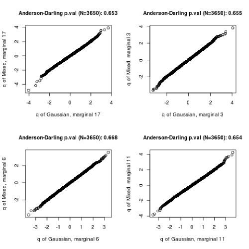
Figure 17: Quantile-quantile plots of four randomly selected components of $\mathbf{Z}$ and $\mathbf{X}$. The p-values of the Anderson-Darling test for equality in distribution (n=3650) are given. The marginal distributions illustrated can be reasonably accepted to be equal.

C.2 Analysis of two dimensional marginal distributions

Data corresponding to two components of both $\mathbf{X}$ and $\mathbf{Z}$, namely 3 and 28, are shown at figure 18 for illustration. The multivariate version of Shapiro-Wilks test for normality introduced by Villasenor Alva and Estrada [2009], as implemented in the R package mvShapiro.Test, was applied to a randomly selected sample (n=500) of $\left(X_{3},X_{28}\right)$. This test resulted in a p-value of $0.191$, whereby $\left(X_{3},X_{28}\right)$ can be considered a Gaussian 2-dimensional vector. The same test procedure was performed on all ${30\choose 2}=435$ pairs of marginals, for $\mathbf{Z}$, $\mathbf{X}$ and $\mathbf{W}$. The results are summarized at table 4. It can be seen that non-Gaussian vectors, $\mathbf{X}$ and $\mathbf{W}$, exhibit Gaussian bivariate marginals most of the time. Results are qualitatively similar to those of $\mathbf{Z}$, in particular for $\mathbf{W}$.

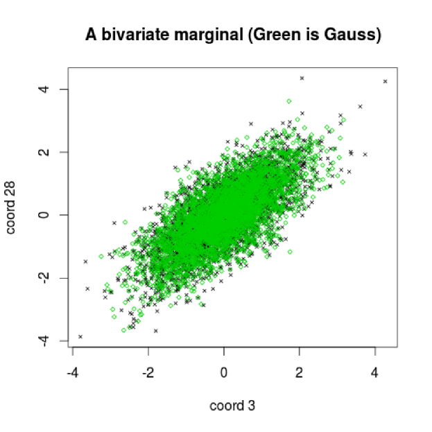
Figure 18: Dispersion plot of two typical components of $\mathbf{Z}$ and $\mathbf{X}$. The p-value of the multivariate Shapiro-Wilks test applied to 500 randomly selected samples of $\left(X_{3},X_{28}\right)$ test is 0.191.

$\alpha$-Level	$\left(Z_{j_{1}},Z_{j_{2}}\right)$	$\left(X_{j_{1}},X_{j_{2}}\right)$	$\left(W_{j_{1}},W_{j_{2}}\right)$
0.01	433 (99.54%)	402 (92.41%)	433 (99.54%)
0.05	419 (96.32%)	360 (82.76%)	421 (96.78%)
0.10	398 (91.49%)	323 (74.25%)	405 (93.10%)

Table 4: Summary of multivariate Shapiro-Wilks test applied on all bivariate marginal distributions of $\mathbf{Z}$, $\mathbf{X}$ and $\mathbf{W}$. A random sub-sample (n=500) from the available data was used for each testing. Out of the total ${30\choose 2}=435$ bivariate combinations, the total number (and percentage) of combinations by which the Normality hypothesis cannot be rejected at the respective $\alpha$-level are shown.

A more detailed analysis of the 2-dimensional components of $\mathbf{Z}$ and $\mathbf{X}$, comprises the study of their respective empirical copulas. Data plotted at figure 19 is given, exemplifying for data of vector $\mathbf{X}$, by

$$u_{i,j}=\hat{F}_{j}\left(x_{i,j}\right)$$

where

$$\hat{F}_{j}\left(a\right):=\frac{\#\left\{x_{i,j}:x_{i,j}\leq a\right\}}{n+1}$$

stands for the empirical cumulative distribution function of component $X_{j}$, for $j=1,\ldots,30$, and $i=1,\ldots,n$. Visually, both data sets seem to have the same empirical copula. The test proposed by Kojadinovic and Yan [2011] and implemented for package copula of R, was applied to a randomly selected sub-sample of size n=500 of data from $\left(X_{3},X_{28}\right)$, with the number of multipliers replications set to N=1000. The resulting p-value is 0.955, whereby gaussianity in the underlying copula seems an acceptable hypothesis. Note that this test is already very efficient under sample sizes of n=300 (see Kojadinovic and Yan [2011]).

Figure 19: Empirical copula plots for: (left) data from $\left(Z_{3},Z_{28}\right)$, and (right) data from $\left(X_{3},X_{28}\right)$. The p-value of goodness of fit test for Gaussianity on a randomly selected subsample (n=500) is 0.955.

The same testing procedure was applied to all possible pair-wise combinations of components of $\mathbf{Z}$ and $\mathbf{X}$, as had been done with the multivariate Shapiro-Wilks test. Results are summarized at table 5. Again, the bivariate sub-vectors of $\mathbf{X}$ are most of the time considered to have the Gaussian copula, in a qualitatively similar proportion as the 2-dimensional sub-vectors of $\mathbf{Z}$.

$\alpha$-Level	$\left(Z_{j_{1}},Z_{j_{2}}\right)$	$\left(X_{j_{1}},X_{j_{2}}\right)$
0.01	433 (99.54%)	433 (99.54%)
0.05	413 (94.94%)	416 (95.63%)
0.10	392 (90.11%)	397 (91.26%)

Table 5: Summary of goodness of fit test for the Gaussian copula applied on all bivariate marginal distributions of $\mathbf{Z}$ and $\mathbf{X}$. A random sub-sample (n=500) from the available data was used for each testing. Out of the total ${30\choose 2}=435$ bivariate combinations, the total number (and percentage) of combinations by which the Normality hypothesis cannot be rejected at the respective $\alpha$-level are shown.

We also fitted T-copulas to the data of all 435 pairs of components, using the data available (n=3650). The idea is to find out how many degrees of freedom would be an optimal assignment for each pair of components, both of $\mathbf{Z}$ and of $\mathbf{X}$. The fitting method employed is described at section 4.2 of Demarta and McNeil [2005], and named "method of moments using Kendall’s Tau".

The 5%, 50% and 95% quantiles of the fitted degrees of freedom are shown at table 6. By fitting all data one gets to a T-copula with 500 and 34.62 degrees of freedom for $\mathbf{Z}$ and $\mathbf{X}$, respectively. As seen in section 5.1, however, the tail dependence of $\mathbf{X}$ is comparable to that of a multivariate T distribution with 15 degrees of freedom, a fact totally invisible for the T-copula fitting procedure, even with a sample size of n=3650. Such a tail behavior, which has gone mostly unnoticed in the one and two dimensional marginals (what Geostatistics check!), may have a great impact on the wider field, of which the data from $\mathbf{X}$ constitute but a partial observation. See section 5.4.

D.o.f quantile (%)	$\left(Z_{j_{1}},Z_{j_{2}}\right)$	$\left(X_{j_{1}},X_{j_{2}}\right)$
5%	35.75	17.97
50%	500.00	34.67
95%	500.00	500.00

Table 6: Quantiles of the degrees of freedom fitted to each of the 435 pairs combinations $\left(Z_{j_{1}},Z_{j_{2}}\right)$ and $\left(X_{j_{1}},X_{j_{2}}\right)$. Using all data, the fitted degrees of freedom are 500 and 45.75 for $\mathbf{Z}$ and $\mathbf{X}$, respectively.

C.3 The fitted covariance function

On the basis of the analysis of the one and two dimensional marginal distributions, we deem adequate to fit a multivariate Normal distribution to $\mathbf{Z}$, $\mathbf{X}$ and $\mathbf{W}$.

Since data comes from the Spatial context illustrated at figure 3, we fit covariance matrices, $cov\left(\mathbf{Z}\right)$, $cov\left(\mathbf{X}\right)$ and $cov\left(\mathbf{W}\right)$, using an exponential covariance function. The estimation method was maximum likelihood using the Normal distribution as model. Estimated parameters are shown in table 7, whereas plots of the resulting covariance functions appear at figure 20.

Vector	Mean	Range par.	Nugget	Var
$\mathbf{Z}$	0.007	19.966	0.000	1.000
$\mathbf{X}$	0.006	19.992	0.000	0.992
$\mathbf{W}$	0.006	19.876	0.000	0.994

Table 7: Gaussian field specification, as estimated by maximum likelihood (n=3650), and using the exponential covariance function model.

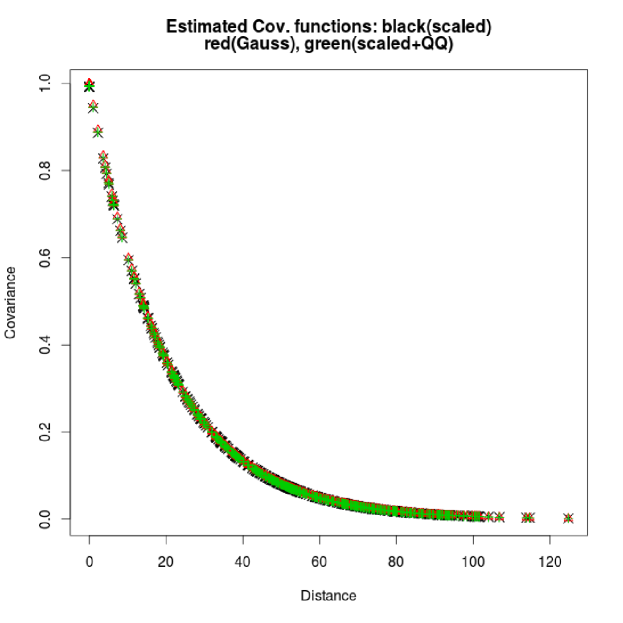
Figure 20: Plots of fitted exponential covariance functions for $\mathbf{Z}$ (red), $\mathbf{X}$ (black) and $\mathbf{W}$ (green). Plots are practically identical.

Note that both the parameter estimates and the covariance function plots are practically identical. As was true during the analysis of the one and two dimensional marginal distributions, there is little evidence that the distributions of $\mathbf{Z}$, $\mathbf{X}$ and $\mathbf{W}$ are not the same. However, the complete fields $\mathbf{X}^{*}\in\mathbb{R}^{90000}$ and $\mathbf{W}^{*}\in\mathbb{R}^{90000}$ are very different from $\mathbf{Z}^{*}\in\mathbb{R}^{90000}$, in terms of important manifestations of interaction.

Appendix D Analysis of Aggregating statistics: statistics to notice the difference

We have seen that both the 1-dimensional and the 2-dimensional marginal distributions of $\mathbf{X}$ and $\mathbf{W}$ seem to indicate that these vectors can be safely modeled by a multivariate Normal model, like the one suitable for $\mathbf{Z}$. We know, however, that the distributions of $\mathbf{Z}$ and $\mathbf{X}$ are not the same.

In this sub-section we compute some statistics that can indicate that the probability distributions of $\mathbf{X}$ and $\mathbf{W}$ may actually be different from that of $\mathbf{Z}$. They aggregate data beyond that of the 2-dimensional marginals. In Rodríguez and Bárdossy [2013] these statistics are called interactions manifestations.

The first aggregating statistic we consider is the number of components trespassing a given threshold $a$. Data observed from $\mathbf{X}$ lead to realizations of random variable $L_{\mathbf{X}}$, defined as

$$L^{\mathbf{X}}=\sum_{j=1}^{J}1\left\{X_{j}>a\right\}$$

where

$$1\left\{X_{j}>a\right\}=\begin{cases}1,&X_{j}>a\\ 0,&X_{j}\leq a\end{cases}$$ (75)

Similar constructions lead to $L^{\mathbf{Z}}$ and $L^{\mathbf{W}}$ from $\mathbf{Z}$ and $\mathbf{W}$, respectively. Denote by $l_{1}^{\mathbf{Z}},\ldots,l_{n}^{\mathbf{Z}}$; $l_{1}^{\mathbf{X}},\ldots,l_{n}^{\mathbf{X}}$ and $l_{1}^{\mathbf{W}},\ldots,l_{n}^{\mathbf{W}}$ the samples of $L^{\mathbf{Z}}$, $L^{\mathbf{X}}$ and $L^{\mathbf{W}}$. These are plotted in figure 21. Note that the difference among the plots begins to be quite apparent for thresholds 2.326 through 3.09. As opposed to what was seen when analyzing the one and two dimensional marginals separately, there seems to be a difference among the distributions of $L^{\mathbf{Z}}$, $L^{\mathbf{X}}$ and $L^{\mathbf{W}}$, and hence of $\mathbf{X}$, $\mathbf{Z}$ and $\mathbf{W}$.

Figure 21: Boxplots of number of components trespassing the four thresholds indicated (1.645, 2.326, 2.576 and 3.09), for samples from $\mathbf{Z}$ (left), $\mathbf{X}$ (middle) and $\mathbf{Z}$ (right). Data has been jittered for visualization purposes. The difference among the plots becomes most apparent as the threshold is pulled up.

The second statistic we mention, is the "congregation measure" used by Bárdossy and Pegram [2009] and Bárdossy and Pegram [2012], for the sake of model validation. This is a measure not affected by monotonic transformations on the components of the vector analyzed.

The congregation measure referred to is constructed as follows. Set a threshold percentile, $b\in\left(0,1\right)$. Select a set of indexes $\left(j_{i_{1}},\ldots j_{i_{K}}\right)$, with $1\leq j_{i_{1}}<\ldots<j_{i_{K}}\leq J$. For the analysis of the components of $\mathbf{X}$, define binary random variables

$$\varsigma_{b}\left(j_{i_{k}}\right)=\begin{cases}1,&F_{j_{i_{k}}}\left(X_{j_{i_{k}}}\right)>b\\ 0,&F_{j_{i_{k}}}\left(X_{j_{i_{k}}}\right)\leq b\end{cases}$$ (76)

This results in a discrete random vector $\varsigma_{b}=\left(\varsigma_{b}\left(j_{i_{1}}\right),\ldots,\varsigma_{b}\left(j_{i_{K}}\right)\right)$. The congregation measure referred to is defined to be the entropy of a sub-vector of $\varsigma$,

$$congr_{b}\left(X_{j_{i_{1}}},\ldots,X_{j_{i_{K}}}\right)=\\ -\sum_{j_{i_{1}},\ldots,j_{i_{K}}}\Pr\left(\varsigma_{b}\left(j_{i_{1}}\right),\ldots,\varsigma_{b}\left(j_{i_{K}}\right)\right)\log\left(\Pr\left(\varsigma_{b}\left(j_{i_{1}}\right),\ldots,\varsigma_{b}\left(j_{i_{K}}\right)\right)\right)$$ (77)

That is, the measure is defined as the entropy of the joint distribution of the binary variables just defined. A higher value of this measure indicates less association. A similar definition applies to $congr_{b}\left(Z_{j_{i_{1}}},\ldots,Z_{j_{i_{K}}}\right)$. Note that this measure is not affected by the marginal distributions of the components employed, hence

$$congr_{b}\left(W_{j_{i_{1}}},\ldots,W_{j_{i_{K}}}\right)=congr_{b}\left(X_{j_{i_{1}}},\ldots,X_{j_{i_{K}}}\right)$$

We applied this measure to three components of vectors $\mathbf{Z}$ and $\mathbf{X}$, namely components 3, 28 and 19, of which the former two were visualized at figure 18. We used percentiles $b\in\left\{0.6,0.7,0.8,0.85,0.9,0.95,0.99,0.995,0.999\right\}$, and computed

$$r_{b}=\frac{congr_{b}\left(Z_{j_{i_{1}}},\ldots,Z_{j_{i_{K}}}\right)}{congr_{b}\left(X_{j_{i_{1}}},\ldots,X_{j_{i_{K}}}\right)}$$

The resulting ratio values are shown in figure 22. The estimated association of the components $\left(Z_{3},Z_{28},Z_{19}\right)$, as quantified by this measure, does not seem to decrease considerably as compared to that of $\left(X_{3},X_{28},X_{19}\right)$. A "parametric bootstrap" (see Efron and Tibshirani [1993]) 90% confidence interval has been added for the ratio of the entropies, computed by simulating a Normal sample of size $n=3650$ with zero means and correlation matrix the sample correlation matrix of $\left(Z_{3},Z_{28},Z_{19}\right)$. The procedure is repeated 10000 times to create the confidence interval.

However, as shown in figure 23, if the sample size is increased to n=10000, the association among subvectors of $\mathbf{X}$ can be seen to increase considerably as compared to that of subvectors of $\mathbf{Z}$. In particular this is the case as one approaches the uppermost tail of the 2, 3, 4 and 5-dimensional distributions. Subvectors employed for the evaluation are indicated in figure 23. This was to be expected in view of the uppermost tail of scaling variable $V$, see the right panel of figure 2. Hence, on the basis of the analysis of only three through five components, it is possible to notice a difference in the dependence structure of the fields (compare Bárdossy and Pegram [2009]), provided the sample size is sufficiently large.

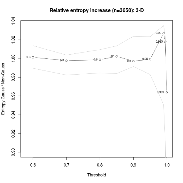
Figure 22: Ratio, $r_{b}$, of congregation measures for the percentiles $b\in\left\{0.6,0.7,0.8,0.85,0.9,0.95,0.99,0.995,0.999\right\}$. Association among the three components $\left(Z_{3},Z_{28},Z_{19}\right)$ decreases considerably as compared to that of $\left(X_{3},X_{28},X_{19}\right)$ from the 99% percentile on. A bootstrap based confidence interval has been added for significance assessment.

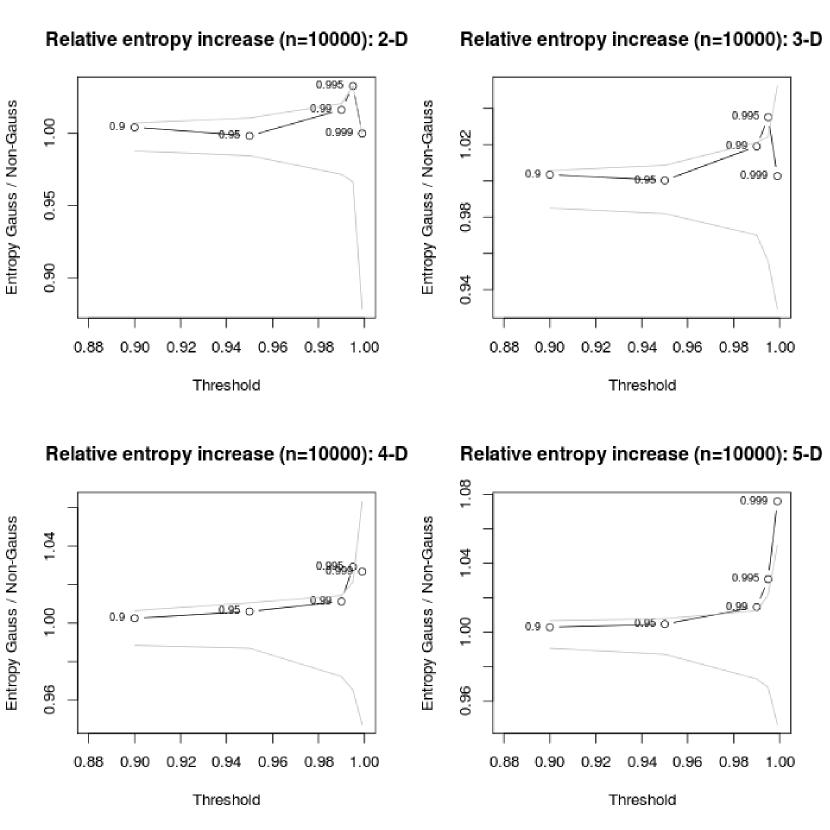
Figure 23: Ratio, $r_{b}$, of congregation measures for the percentiles $b\in\left\{0.6,0.7,0.8,0.85,0.9,0.95,0.99,0.995,0.999\right\}$. Association among two, three, four and five components of $\mathbf{Z}$ decreases considerably as compared to that of subvectors of $\mathbf{X}$ from the 99% percentile on. A bootstrap based confidence intervals have been added for significance assessment. Subvectors used have indexes $\left(3,28\right),\left(3,28,19\right),\left(3,28,19,16\right)$ and $\left(3,28,19,16,25\right)$.

A third kind of aggregating statistic comprises the quantiles of the sum of components above given thresholds. To this end, we took the n=3650 observations of each vector, $\mathbf{Z}$, $\mathbf{X}$ and $\mathbf{W}$, and obtained from them $s_{1}^{\mathbf{Z}},\ldots,s_{n}^{\mathbf{Z}},\ldots,s_{n}^{\mathbf{W}}$. Where, for a given threshold $a$, one has for example,

$$s_{i}^{\mathbf{X}}=\sum_{j=1}^{30}1\left\{x_{ij}>a\right\}\times x_{ij}$$ (78)

with $i=1,\ldots,3650$.

The empirical cumulative distribution functions built from $s_{1}^{\mathbf{X}},\ldots,s_{3650}^{\mathbf{X}}$ and $s_{1}^{\mathbf{W}},\ldots,s_{3650}^{\mathbf{W}}$ are presented in figure 24, for thresholds $a=\left\{1.04,1.28,2.5,3\right\}$. Simulation based 90% confidence intervals (appearing in red) for the empirical cumulative distribution function of $s_{1}^{\mathbf{Z}},\ldots,s_{3650}^{\mathbf{Z}}$ were also added. These confidence intervals were created for each threshold, $a$, by repeting 1000 times the following procedure: simulate n=3650 realizations of a Gaussian random vector with mean and covariance as estimated for $\mathbf{X}$ in section C.3, and then apply construction (78). In this manner we obtain 1000 empirical cumulative distribution functions; at each percentile $u\in\left[0,1\right]$, we compute the values of all 1000 e.c.d.f. and take from them the 5% and 95% quantile values.

It is clear from figure 24, that tails of the distribution functions obtained for $s_{1}^{\mathbf{X}},\ldots,s_{3650}^{\mathbf{X}}$ for thresholds $a\in\left\{2.5,3\right\}$ are heavier than expected from a Gaussian vector having the same means, covariance matrix, and approximately the same marginal distributions as $\mathbf{X}$. Hence, the analysis of these statistics is valuable for diagnosis of higher order interaction.

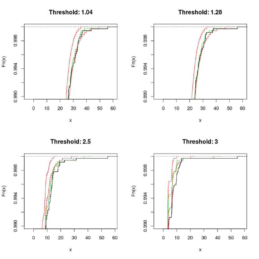
Figure 24: Empirical distributions of sums above various thresholds (1.04, 1.28, 2.5 and 3) for the n=3650 observations of random vectors $\mathbf{X}$ (black) and $\mathbf{W}$ (green). Simulation based 90% confidence intervals for the empirical distributions arising from a Gaussian vector with the same means and covariance matrix as $\mathbf{X}$ appear in red. The tail of the sums above thresholds 2.5 and 3 is significantly heavier than the Gaussian model would prescribe.

Appendix E MCMC estimation of the conditional scaling variable

In the following, $\mathbf{x}\in\mathbb{R}^{J}$ represents a partial observation of a complete field $\left(\mathbf{x},\mathbf{x}^{*}\right)\in\mathbb{R}^{J+M}$. Also, as indicated in section 4.2, $p\left(\mathbf{x}-\mu\mid V\right)$ is just $N_{J}\left(\mathbf{0},V\times\Sigma\right)$, the multivariate Normal distribution on $\mathbb{R}^{J}$ with vector of means $\mathbf{0}$ and covariance matrix $V\times\Sigma$.

We can build a Markov Chain whose stationary distribution is approximately that of $V\mid\mathbf{x},\Sigma,\mu$, as follows:

1. Provide an initial value for the Markov chain, say, $V^{\left(0\right)}=1$.

2. For $b=1,\ldots,B$, do:

   1. Sample a candidate value $C^{\left(b\right)}\sim N\left(V^{\left(b-1\right)},1\right)$. A variance of 1 for the transition kernel seems to be adequate for most cases, according to initial exploratory analyses.

   2. If $C^{\left(b\right)}\leq 0$, set $V^{\left(b\right)}=V^{\left(b-1\right)}$. Proceed to iteration $b+1$.

   3. If $C^{\left(b\right)}>0$, compute $w=\frac{p\left(\mathbf{x}-\mu\mid C^{\left(b\right)}\right)p\left(C^{\left(b\right)}\right)}{p\left(\mathbf{x}-\mu\mid V^{\left(b-1\right)}\right)p\left(V^{\left(b.1\right)}\right)}$ and sample $U\sim Unif\left(0,1\right)$. Set $V^{\left(b\right)}=C^{\left(b\right)}$ if $U<\frac{p\left(\mathbf{\mathbf{x}}-\mu\mid C^{\left(b\right)}\right)p\left(C^{\left(b\right)}\right)}{p\left(\mathbf{x}-\mu\mid V^{\left(b-1\right)}\right)p\left(V^{\left(b.1\right)}\right)}$, else set $V^{\left(b\right)}=V^{\left(b-1\right)}$. Proceed to iteration $b+1$.

After sufficiently many iterations, the values $V^{\left(b\right)}$ can be considered as correlated samples from $p\left(V\mid\mathbf{y}-\mu\right)$. After convergence of the Markov Chain just built, we store additional $B$ samples $V^{\left(1\right)},\ldots,V^{\left(B\right)}$. We use these additional samples for conditionally simulating from the total field, $\left(\mathbf{X},\mathbf{X}^{*}\right)$, in the presence of observed data, $\mathbf{X}=\mathbf{x}$.

References

References

- Abramowitz [1972] Abramowitz, M., 1972. Handbook of Mathematical Functions: with formulas, graphs, and mathematical tables. Dover Publications, New York.
- Banerjee et al. [2003] Banerjee, S., Gelfand, A.E., Carlin, B.P., 2003. Hierarchical modeling and analysis for spatial data. CRC Press.
- Bárdossy and Pegram [2009] Bárdossy, A., Pegram, G., 2009. Copula based multisite model for daily precipitation simulation. Hydrology and Earth System Sciences Discussions 6, 4485–4534. URL: http://www.hydrol-earth-syst-sci-discuss.net/6/4485/2009/, doi:10.5194/hessd-6-4485-2009.
- Bárdossy and Pegram [2012] Bárdossy, A., Pegram, G., 2012. Multiscale spatial recorrelation of RCM precipitation to produce unbiased climate change scenarios over large areas and small. Water Resources Research 48. URL: http://www.agu.org/pubs/crossref/2012/2011WR011524.shtml, doi:10.1029/2011WR011524.
- Barndorff-Nielsen and Cox [1990] Barndorff-Nielsen, O.E., Cox, D.R., 1990. Asymptotic techniques for use in statistics. Chapman and Hall, London [u.a.].
- Cambanis et al. [1981] Cambanis, S., Huang, S., Simons, G., 1981. On the theory of elliptically contoured distributions. Journal of Multivariate Analysis 11, 368 – 385. URL: http://www.sciencedirect.com/science/article/pii/0047259X81900828, doi:10.1016/0047-259X(81)90082-8.
- Cressie and Wikle [2011] Cressie, N., Wikle, C.K., 2011. Statistics for spatio-temporal data. Wiley.
- Cressie [1991] Cressie, N.A.C., 1991. Statistics for spatial data. Wiley series in probability and mathematical statistics, Wiley, New York.
- Del Brio et al. [2009] Del Brio, E.B., Ñiguez, T.M., Perote, J., 2009. Gram-Charlier densities: a multivariate approach. Quantitative Finance 9, 855–868. URL: http://www.tandfonline.com/doi/abs/10.1080/14697680902773611, doi:10.1080/14697680902773611.
- Demarta and McNeil [2005] Demarta, S., McNeil, A.J., 2005. The t copula and related copulas. International Statistical Review 73, 111–129. URL: http://dx.doi.org/10.1111/j.1751-5823.2005.tb00254.x, doi:10.1111/j.1751-5823.2005.tb00254.x.
- Diggle and Ribeiro [2007] Diggle, P.J., Ribeiro, P.J., 2007. Model-based Geostatistics. Springer.
- Efron and Tibshirani [1993] Efron, B., Tibshirani, R., 1993. An introduction to the bootstrap. volume 57. CRC press.
- Gallant and Nychka [1987] Gallant, A.R., Nychka, D.W., 1987. Semi-nonparametric maximum likelihood estimation. Econometrica 55, pp. 363–390. URL: http://www.jstor.org/stable/1913241.
- Kano [1994] Kano, Y., 1994. Consistency property of elliptic probability density functions. Journal of Multivariate Analysis 51, 139 – 147. URL: http://www.sciencedirect.com/science/article/pii/S0047259X84710542, doi:http://dx.doi.org/10.1006/jmva.1994.1054.
- Kendall and Stuart [1969] Kendall, M.G., Stuart, A., 1969. The advanced theory of statistics Vol. 1, Distribution theory. Griffin, London.
- Kleiber et al. [2012] Kleiber, W., Katz, R.W., Rajagopalan, B., 2012. Daily spatiotemporal precipitation simulation using latent and transformed gaussian processes. Water Resources Research 48, n/a–n/a. URL: http://dx.doi.org/10.1029/2011WR011105, doi:10.1029/2011WR011105.
- Kojadinovic and Yan [2011] Kojadinovic, I., Yan, J., 2011. A goodness-of-fit test for multivariate multiparameter copulas based on multiplier central limit theorems. Statistics and Computing 21, 17–30.
- Kolassa [2006] Kolassa, J., 2006. Series approximation methods in statistics. volume 88. Springer.
- Kolassa and Li [2010] Kolassa, J., Li, J., 2010. Multivariate saddlepoint approximations in tail probability and conditional inference. Bernoulli 16, 1191–1207.
- Kolassa and Tanner [1994] Kolassa, J.E., Tanner, M.A., 1994. Approximate conditional inference in exponential families via the gibbs sampler. Journal of the American Statistical association 89, 697–702.
- Kotz and Nadarajah [2004] Kotz, S., Nadarajah, S., 2004. Multivariate t-distributions and their applications. Cambridge University Press.
- Le and Zidek [2006] Le, N.D., Zidek, J.V., 2006. Statistical analysis of environmental space-time processes. Springer series in statistics, Springer, New York.
- Mauleon and Perote [2000] Mauleon, I., Perote, J., 2000. Testing densities with financial data: an empirical comparison of the Edgeworth–Sargan density to the student t. The European Journal of Finance 6, 225–239.
- Perote [2004] Perote, J., 2004. The multivariate Edgeworth–Sargan density. Spanish Economic Review 6, 77–96. URL: http://link.springer.com/10.1007/s10108-003-0075-x, doi:10.1007/s10108-003-0075-x.
- Ripley [1981] Ripley, B.D., 1981. Spatial statistics. Wiley series in probability and mathematical statistics, Wiley, New York.
- Rodríguez and Bárdossy [2013] Rodríguez, J., Bárdossy, A., 2013. Modeling of multivariate interactions through their manifestations and low dimensional model building via the Cumulant Generating Function. Technical Report. Institute for Modelling Hydraulic and Environmental Systems, Universität Stuttgart.
- Sansó and Guenni [1999] Sansó, B., Guenni, L., 1999. Venezuelan rainfall data analysed by using a bayesian space-time model. Journal of the Royal Statistical Society: Series C (Applied Statistics) 48, 345–362. URL: http://doi.wiley.com/10.1111/1467-9876.00157, doi:10.1111/1467-9876.00157.
- Skovgaard [1987] Skovgaard, I., 1987. Saddlepoint expansions for conditional distributions. Journal of Applied Probability , 875–887.
- Smith [1995] Smith, P.J., 1995. A recursive formulation of the old problem of obtaining moments from cumulants and vice versa. The American Statistician 49, 217–218.
- Steyn [1993] Steyn, H., 1993. On the problem of more than one kurtosis parameter in multivariate analysis. Journal of Multivariate Analysis 44, 1 – 22. URL: http://www.sciencedirect.com/science/article/pii/S0047259X83710018, doi:10.1006/jmva.1993.1001.
- Villasenor Alva and Estrada [2009] Villasenor Alva, J.A., Estrada, E.G., 2009. A generalization of shapiro–wilk’s test for multivariate normality. Communications in Statistics Theory and Methods 38, 1870–1883.